Mapping Heat-Related Risks in Northern Jiangxi Province of China Based on Two Spatial Assessment Frameworks Approaches

 ,
,  , and
, and
Abstract
1. Introduction
2. Materials and Methods
2.1. Study Area
2.2. Data Collection and Preprocessing
2.2.1. Land Surface Temperature
2.2.2. Counties’ Air Temperature
2.2.3. Wet Bulb Globe Temperature
2.2.4. Air Quality Index Data
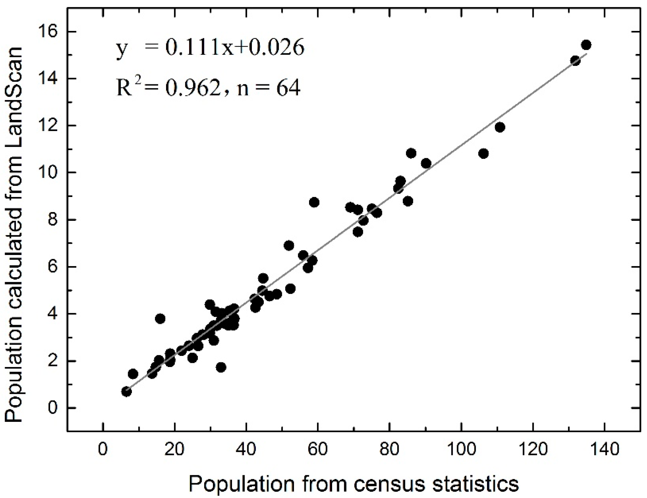
2.2.5. Socio-Economical and Statistical Data
2.2.6. Proximity to Vegetation
2.2.7. Terrain Data
2.2.8. Proximity to Water
2.3. Methods
2.3.1. Heat Hazard and Exposure
2.3.2. Heat Exposure and Sensibility
2.3.3. Heat Vulnerability and Adaptability
2.3.4. Heat Risk and Vulnerability
3. Results
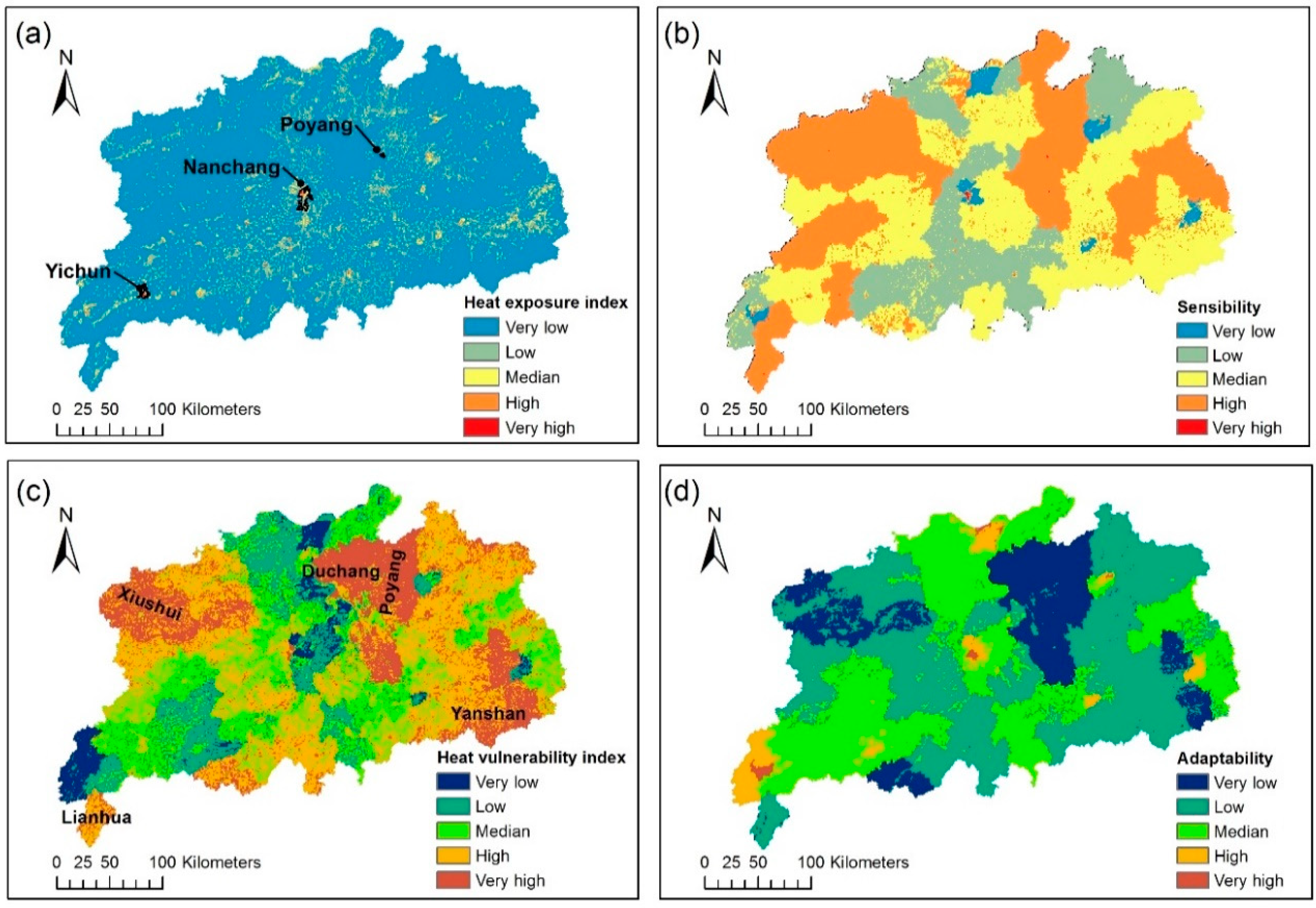
3.1. Heat Hazard and Exposure
3.2. Heat Exposure and Sensitivity
3.3. Heat Vulnerablity and Adaptability
3.4. Heat Risk and Vulnerability
4. Discussion
5. Conclusions
Author Contributions
Funding
Acknowledgments
Conflicts of Interest
Appendix A


Appendix B

| IAQI | SO2 | NO2 | PM10 | CO | O3 | PM2.5 |
|---|---|---|---|---|---|---|
| μg/m3 | μg/m3 | μg/m3 | μg/m3 | μg/m3 | μg/m3 | |
| 0 | 0 | 0 | 0 | 0 | 0 | 0 |
| 50 | 50 | 40 | 50 | 2 | 100 | 35 |
| 100 | 150 | 80 | 150 | 4 | 160 | 75 |
| 150 | 475 | 180 | 250 | 14 | 215 | 115 |
| 200 | 800 | 280 | 350 | 24 | 265 | 150 |
| 300 | 1600 | 565 | 420 | 36 | 800 | 250 |
| 400 | 2100 | 750 | 500 | 48 | >800 | 350 |
| 500 | 2620 | 940 | 600 | 60 | >800 | 500 |
| AQI | Level | Description |
|---|---|---|
| <50 | I | Excellent |
| 0 | II | Good |
| 50 | III | Mild pollution |
| 100 | IV | Medium pollution |
| 150 | V | Heavy pollution |
| 200 | VI | Severe pollution |
Appendix C
| Urban 1 | Test of Normality | Wilcoxon Signed Rank Test | |||
| statistic | df | sig. | standardized test statistics | sig. | |
| HVI-heat risk index 1 | 0.79 | 26 | 0.00 | 4.46 | 0.00 |
| Urban 2 | Test of normality | Wilcoxon signed rank test | |||
| statistic | df | sig. | standardized test statistics | sig. | |
| HVI-heat risk index | 0.88 | 52 | 0.00 | 6.28 | 0.00 |
| Urban 3 | Test of normality | Wilcoxon signed rank test | |||
| statistic | df | sig. | standardized test statistics | sig. | |
| HVI-heat risk index | 0.96 | 70 | 0.01 | 7.27 | 0.00 |
| Urban 4 | Test of normality | Wilcoxon signed rank test | |||
| statistic | df | sig. | standardized test statistics | sig. | |
| HVI-heat risk index | 0.86 | 35 | 0.00 | 5.16 | 0.00 |
| Urban 5 | Test of normality | Paired sample T-test | |||
| statistic | df | sig. | t | sig. | |
| HVI-heat risk index | 0.98 | 15 | 0.94 | 94.34 | 0.00 |
| Urban 6 | Test of normality | Mann-Whitney U test | |||
| statistic | df | sig. | standardized test statistics | sig. | |
| HVI | 0.88 | 33 | 0.00 | 6.98 | 0.00 |
| heat risk index | 0.70 | 33 | 0.00 | ||
| Urban 7 | Test of normality | Wilcoxon signed rank test | |||
| statistic | df | sig. | standardized test statistics | sig. | |
| HVI-heat risk index | 0.87 | 182 | 0.00 | 11.70 | 0.00 |
| Urban 8 | Test of normality | Wilcoxon signed rank test | |||
| statistic | df | sig. | standardized test statistics | sig. | |
| HVI-heat risk index | 0.78 | 46 | 0.00 | 5.91 | 0.00 |
| Urban 9 | Test of normality | Paired sample T-test | |||
| statistic | df | sig. | t | sig. | |
| HVI-heat risk index | 0.97 | 36 | 0.33 | 6.72 | 0.00 |
References
- Mishra, V.; Ganguly, A.R.; Nijssen, B.; Lettenmaier, D.P. Changes in observed climate extremes in global urban areas. Environ. Res. Lett. 2015, 10, 024005. [Google Scholar] [CrossRef]
- Perkins, S.E.; Alexander, L.V.; Nairn, J.R. Increasing frequency, intensity and duration of observed global heatwaves and warm spells. Geophys. Res. Lett. 2012, 39, 1–5. [Google Scholar] [CrossRef]
- Semenza, J.C.; Rubin, C.H.; Falter, K.H.; Selanikio, J.D.; Flanders, W.D.; Howe, H.L.; Wilhelm, J.L. Heat-related deaths during the July 1995 heat wave in Chicago. N. Engl. J. Med. 1996, 335, 84–90. [Google Scholar] [CrossRef]
- Kovats, R.S.; Ebi, K.L. Heatwaves and public health in Europe. Eur. J. Public Health 2006, 16, 592–599. [Google Scholar] [CrossRef] [PubMed]
- Shaposhnikov, D.; Revich, B.; Bellander, T.; Bedada, G.B.; Bottai, M.; Kharkova, T.; Kvasha, E.; Lezina, E.; Lind, T.; Semutnikova, E.; et al. Mortality Related to Air Pollution with the Moscow Heat Wave and Wildfire of 2010. Epidemiology 2014, 25, 359–364. [Google Scholar] [CrossRef]
- Mora, C.; Dousset, B.; Caldwell, I.R.; Powell, F.E.; Geronimo, R.C.; Bielecki, C.R.; Counsell, C.W.W.; Dietrich, B.S.; Johnston, E.T.; Louis, L.V.; et al. Global risk of deadly heat. Nat. Clim. Chang. 2017, 7, 501–506. [Google Scholar] [CrossRef]
- Song, J.; Huang, B.; Kim, J.S.; Wen, J.; Li, R. Fine-scale mapping of an evidence-based heat health risk index for high-density cities: Hong Kong as a case study. Sci. Total Environ. 2020, 718, 137226. [Google Scholar] [CrossRef]
- Zhang, W.; Zheng, C.; Chen, F. Mapping heat-related health risks of elderly citizens in mountainous area: A case study of Chongqing, China. Sci. Total Environ. 2019, 663, 852–866. [Google Scholar] [CrossRef] [PubMed]
- Chen, Q.; Ding, M.; Yang, X.; Hu, K.; Qi, J. Spatially explicit assessment of heat health risk by using multi-sensor remote sensing images and socioeconomic data in Yangtze River Delta, China. Int. J. Health Geogr. 2018, 17, 15. [Google Scholar] [CrossRef]
- Buscail, C.; Upegui, E.; Viel, J.F. Mapping heatwave health risk at the community level for public health action. Int. J. Health Geogr. 2012, 11, 1–9. [Google Scholar] [CrossRef]
- He, C.; Ma, L.; Zhou, L.; Kan, H.D.; Zhang, Y.; Ma, W.C.; Chen, B. Exploring the mechanisms of heat wave vulnerability at the urban scale based on the application of big data and artificial societies. Environ. Int. 2019, 127, 573–583. [Google Scholar] [CrossRef] [PubMed]
- Hu, K.; Yang, X.; Zhong, J.; Fei, F.; Qi, J. Spatially Explicit Mapping of Heat Health Risk Utilizing Environmental and Socioeconomic Data. Environ. Sci. Technol. 2017, 51, 1498–1507. [Google Scholar] [CrossRef] [PubMed]
- Heaton, M.J.; Sain, S.R.; Greasby, T.A.; Uejio, C.K.; Hayden, M.H.; Monaghan, A.J.; Boehnert, J.; Sampson, K.; Banerjee, D.; Nepal, V.; et al. Characterizing urban vulnerability to heat stress using a spatially varying coefficient model. Spat. Spatiotemporal. Epidemiol. 2014, 8, 23–33. [Google Scholar] [CrossRef] [PubMed]
- Wolf, T.; McGregor, G. The development of a heat wave vulnerability index for London, United Kingdom. Weather Clim. Extrem. 2013, 1, 59–68. [Google Scholar] [CrossRef]
- Harlan, S.L.; Declet-Barreto, J.H.; Stefanov, W.L.; Petitti, D.B. Neighborhood effects on heat deaths: Social and environmental predictors of vulnerability in Maricopa county, Arizona. Environ. Health Perspect. 2013, 121, 197–204. [Google Scholar] [CrossRef] [PubMed]
- Zhang, W.; McManus, P.; Duncan, E. A raster-based subdividing indicator to map urban heat vulnerability: A case study in sydney, australia. Int. J. Environ. Res. Public Health 2018, 15, 2516. [Google Scholar] [CrossRef] [PubMed]
- Hulley, G.; Shivers, S.; Wetherley, E.; Cudd, R. New ECOSTRESS and MODIS land surface temperature data reveal fine-scale heat vulnerability in cities: A case study for Los Angeles County, California. Remote Sens. 2019, 11, 2136. [Google Scholar] [CrossRef]
- Maier, G.; Grundstein, A.; Jang, W.; Li, C.; Naeher, L.P.; Shepherd, M. Assessing the performance of a vulnerability index during oppressive heat across georgia, United States. Weather. Clim. Soc. 2014, 6, 253–263. [Google Scholar] [CrossRef]
- Cai, Z.; Tang, Y.; Chen, K.; Han, G. Assessing the heat vulnerability of different local climate zones in the old areas of a Chinese megacity. Sustainability 2019, 11, 2032. [Google Scholar] [CrossRef]
- Azhar, G.; Saha, S.; Ganguly, P.; Mavalankar, D.; Madrigano, J. Heat wave vulnerability mapping for India. Int. J. Environ. Res. Public Health 2017, 14, 357. [Google Scholar] [CrossRef]
- Rinner, C.; Patychuk, D.; Bassil, K.; Nasr, S.; Gower, S.; Campbell, M. The role of maps in neighborhood-level heat vulnerability assessment for the city of toronto. Cartogr. Geogr. Inf. Sci. 2010, 37, 31–44. [Google Scholar] [CrossRef]
- Zhu, Q.; Liu, T.; Lin, H.; Xiao, J.; Luo, Y.; Zeng, W.; Zeng, S.; Wei, Y.; Chu, C.; Baum, S.; et al. The spatial distribution of health vulnerability to heat waves in guangdong province, China. Glob. Health Action 2014, 7, 25051. [Google Scholar] [CrossRef] [PubMed]
- Inostroza, L.; Palme, M.; De La Barrera, F. A heat vulnerability index: Spatial patterns of exposure, sensitivity and adaptive capacity for Santiago de Chile. PLoS ONE 2016, 11, e0162464. [Google Scholar] [CrossRef] [PubMed]
- Fedeski, M.; Gwilliam, J. Urban sustainability in the presence of flood and geological hazards: The development of a GIS-based vulnerability and risk assessment methodology. Landsc. Urban Plan. 2007, 83, 50–61. [Google Scholar] [CrossRef]
- Gwilliam, J.; Fedeski, M.; Lindley, S.; Theuray, N.; Handley, J. Methods for assessing risk from climate hazards in urban areas. Proc. Inst. Civ. Eng. Eng. 2006, 159, 245–255. [Google Scholar] [CrossRef]
- Bai, L.; Woodward, A.; Liu, Q. County-level heat vulnerability of urban and rural residents in Tibet, China. Environ. Health 2016, 15, 3. [Google Scholar] [CrossRef]
- Crichton, D. The risk triangle. In Natural Disaster Management; Ingleton, J., Ed.; Tudor Rose: London, UK, 1999; pp. 102–103. ISBN 0-9536140-1-8. [Google Scholar]
- Tomlinson, C.J.; Chapman, L.; Thornes, J.E.; Baker, C.J. Including the urban heat island in spatial heat health risk assessment strategies: A case study for Birmingham, UK. Int. J. Health Geogr. 2011, 10, 1–14. [Google Scholar] [CrossRef]
- Coutts, A.M.; Beringer, J.; Tapper, N.J. Impact of increasing urban density on local climate: Spatial and temporal variations in the surface energy balance in Melbourne, Australia. J. Appl. Meteorol. Climatol. 2007, 46, 477–493. [Google Scholar] [CrossRef]
- Wilhelmi, O.V.; Hayden, M.H. Connecting people and place: A new framework for reducing urban vulnerability to extreme heat. Environ. Res. Lett. 2010, 5, 014021. [Google Scholar] [CrossRef]
- Reid, C.E.; O’Neill, M.S.; Gronlund, C.J.; Brines, S.J.; Brown, D.G.; Diez-Roux, A.V.; Schwartz, J. Mapping Community Determinants of Heat Vulnerability. Environ. Health Perspect. 2009, 117, 1730–1736. [Google Scholar] [CrossRef]
- Ho, H.C.; Knudby, A.; Chi, G.; Aminipouri, M.; Lai, D.Y.-F. Spatiotemporal analysis of regional socio-economic vulnerability change associated with heat risks in Canada. Appl. Geogr. 2018, 95, 61–70. [Google Scholar] [CrossRef] [PubMed]
- Faisal, K.; Shaker, A. An Investigation of GIS Overlay and PCA Techniques for Urban Environmental Quality Assessment: A Case Study in Toronto, Ontario, Canada. Sustainability 2017, 9, 380. [Google Scholar] [CrossRef]
- Nayak, S.G.; Shrestha, S.; Kinney, P.L.; Ross, Z.; Sheridan, S.C.; Pantea, C.I.; Hsu, W.H.; Muscatiello, N.; Hwang, S.A. Development of a heat vulnerability index for New York State. Public Health 2018, 161, 127–137. [Google Scholar] [CrossRef] [PubMed]
- Vandentorren, S.; Bretin, P.; Zeghnoun, A.; Mandereau-Bruno, L.; Croisier, A.; Cochet, C.; Riberon, J.; Siberan, I.; Declercq, B.; Ledrans, M. August 2003 heat wave in France: Risk factors for death of elderly people living at home. Eur. J. Public Health 2006, 16, 583–591. [Google Scholar] [CrossRef] [PubMed]
- Tan, J. Commentary: Peoples vulnerability to heat wave. Int. J. Epidemiol. 2008, 37, 318–320. [Google Scholar] [CrossRef]
- Conti, S.; Meli, P.; Minelli, G.; Solimini, R.; Toccaceli, V.; Vichi, M.; Beltrano, C.; Perini, L. Epidemiologic study of mortality during the Summer 2003 heat wave in Italy. Environ. Res. 2005, 98, 390–399. [Google Scholar] [CrossRef]
- Grize, L.; Huss, A.; Thommen, O.; Schindler, C.; Braun-Fabrlander, C. Heat wave 2003 and mortality in Switzerland. SWISS Med. Wkly. 2005, 135, 200–205. [Google Scholar]
- Wang, D.; Lau, K.K.-L.; Ren, C.; Goggins, W.B.I.I.; Shi, Y.; Ho, H.C.; Lee, T.-C.; Lee, L.-S.; Woo, J.; Ng, E. The impact of extremely hot weather events on all-cause mortality in a highly urbanized and densely populated subtropical city: A 10-year time-series study (2006–2015). Sci. Total Environ. 2019, 690, 923–931. [Google Scholar] [CrossRef]
- Huynen, M.; Martens, P.; Schram, D.; Weijenberg, M.P.; Kunst, A.E. The impact of heat waves and cold spells on mortality rates in the Dutch population. Environ. Health Perspect. 2001, 109, 463–470. [Google Scholar] [CrossRef]
- Flynn, A.; McGreevy, C.; Mulkerrin, E.C. Why do older patients die in a heatwave? QJM-AN Int. J. Med. 2005, 98, 227–229. [Google Scholar] [CrossRef]
- Sheffield, P.E.; Landrigan, P.J. Global Climate Change and Children’s Health: Threats and Strategies for Prevention. Environ. Health Perspect. 2011, 119, 291–298. [Google Scholar] [CrossRef] [PubMed]
- Basu, R. High ambient temperature and mortality: A review of epidemiologic studies from 2001 to 2008. Environ. Health 2009, 8, 40. [Google Scholar] [CrossRef] [PubMed]
- Xu, Z.; Etzel, R.A.; Su, H.; Huang, C.; Guo, Y.; Tong, S. Impact of ambient temperature on children’s health: A systematic review. Environ. Res. 2012, 117, 120–131. [Google Scholar] [CrossRef] [PubMed]
- Mendez-Lazaro, P.; Muller-Karger, F.E.; Otis, D.; McCarthy, M.J.; Rodriguez, E. A heat vulnerability index to improve urban public health management in San Juan, Puerto Rico. Int. J. Biometeorol. 2018, 62, 709–722. [Google Scholar] [CrossRef] [PubMed]
- Duzinski, S.V.; Barczyk, A.N.; Wheeler, T.C.; Iyer, S.S.; Lawson, K.A. Threat of paediatric hyperthermia in an enclosed vehicle: A year-round study. Inj. Prev. 2014, 20, 220–225. [Google Scholar] [CrossRef] [PubMed]
- Yin, P.; Chen, R.; Wang, L.; Liu, C.; Niu, Y.; Wang, W.; Jiang, Y.; Liu, Y.; Liu, J.; Qi, J.; et al. The added effects of heatwaves on cause-specific mortality: A nationwide analysis in 272 Chinese cities. Environ. Int. 2018, 121, 898–905. [Google Scholar] [CrossRef]
- Chen, K.; Zhou, L.; Chen, X.; Ma, Z.; Liu, Y.; Huang, L.; Bi, J.; Kinney, P.L. Urbanization Level and Vulnerability to Heat-Related Mortality in Jiangsu Province, China. Environ. Health Perspect. 2016, 124, 1863–1869. [Google Scholar] [CrossRef]
- Marchetti, E.; Capone, P.; Freda, D. Climate change impact on microclimate of work environment related to occupational health and productivity. Ann. DELL Ist. Super. Sanita 2016, 52, 338–342. [Google Scholar]
- Yu, S.; Xia, J.; Yan, Z.; Zhang, A.; Xia, Y.; Guan, D.; Han, J.; Wang, J.; Chen, L.; Liu, Y. Loss of work productivity in a warming world: Differences between developed and developing countries. J. Clean. Prod. 2019, 208, 1219–1225. [Google Scholar] [CrossRef]
- Nunfam, V.F.; Adusei-Asante, K.; Van Etten, E.J.; Oosthuizen, J.; Frimpong, K. Social impacts of occupational heat stress and adaptation strategies of workers: A narrative synthesis of the literature. Sci. Total Environ. 2018, 643, 1542–1552. [Google Scholar] [CrossRef]
- Dong, W.; Liu, Z.; Zhang, L.; Tang, Q.; Liao, H.; Li, X. Assessing heat health risk for sustainability in Beijing’s urban heat island. Sustainability 2014, 6, 7334–7357. [Google Scholar] [CrossRef]
- Heo, S.; Bell, M.L.; Lee, J.T. Comparison of health risks by heat wave definition: Applicability of wet-bulb globe temperature for heat wave criteria. Environ. Res. 2019, 168, 158–170. [Google Scholar] [CrossRef] [PubMed]
- Sheridan, S.C.; Allen, M.J. Temporal trends in human vulnerability to excessive heat. Environ. Res. Lett. 2018, 13, 043001. [Google Scholar] [CrossRef]
- Hoffmann, B.; Hertel, S.; Boes, T.; Weiland, D.; Joeckel, K.-H. Increased cause-specific mortality associated with 2003 heat wave in Essen, Germany. J. Toxicol. Environ. Health Curr. Issues 2008, 71, 759–765. [Google Scholar] [CrossRef]
- Son, J.-Y.; Lee, J.-T.; Anderson, G.B.; Bell, M.L. The Impact of Heat Waves on Mortality in Seven Major Cities in Korea. Environ. Health Perspect. 2012, 120, 566–571. [Google Scholar] [CrossRef]
- Wu, P.-C.; Lin, C.-Y.; Lung, S.-C.; Guo, H.-R.; Chou, C.-H.; Su, H.-J. Cardiovascular mortality during heat and cold events: Determinants of regional vulnerability in Taiwan. Occup. Environ. Med. 2011, 68, 525–530. [Google Scholar] [CrossRef]
- Henderson, S.B.; Wan, V.; Kosatsky, T. Differences in heat-related mortality across four ecological regions with diverse urban, rural, and remote populations in British Columbia, Canada. Health Place 2013, 23, 48–53. [Google Scholar] [CrossRef]
- Wang, Y.; Liu, Y.; Ye, D.; Li, N.; Bi, P.; Tong, S.; Wang, Y.; Cheng, Y.; Li, Y.; Yao, X. High temperatures and emergency department visits in 18 sites with different climatic characteristics in China: Risk assessment and attributable fraction identification. Environ. Int. 2020, 136, 105486. [Google Scholar] [CrossRef]
- Huang, J.; Li, G.; Liu, Y.; Huang, J.; Xu, G.; Qian, X.; Cen, Z.; Pan, X.; Xu, A.; Guo, X.; et al. Projections for temperature-related years of life lost from cardiovascular diseases in the elderly in a Chinese city with typical subtropical climate. Environ. Res. 2018, 167, 614–621. [Google Scholar] [CrossRef]
- Zhang, J.H.; Yao, F.M.; Li, B.B.; Yan, H.; Hou, Y.Y.; Cheng, G.F.; Boken, V. Progress in monitoring high-temperature damage to rice through satellite and ground-based optical remote sensing. Sci. China Earth Sci. 2011, 54, 1801–1811. [Google Scholar] [CrossRef]
- Li, L.; Zha, Y. Population exposure to extreme heat in China: Frequency, intensity, duration and temporal trends. Sustain. Cities Soc. 2020, 60, 102282. [Google Scholar] [CrossRef]
- Hu, L.; Huang, G.; Qu, X. Spatial and temporal features of summer extreme temperature over China during 1960–2013. Theor. Appl. Climatol. 2017, 128, 821–833. [Google Scholar] [CrossRef]
- Deng, K.; Yang, S.; Ting, M.; Zhao, P.; Wang, Z. Dominant Modes of China Summer Heat Waves Driven by Global Sea Surface Temperature and Atmospheric Internal Variability. J. Clim. 2019, 32, 3761–3775. [Google Scholar] [CrossRef]
- Weather Website. Available online: https://lishi.tianqi.com/ (accessed on 26 July 2019).
- Błazejczyk, K. BioKlima—Universal Tool for Bioclimatic and Thermophysiological—Studies. 2017. Available online: https://www.igipz.pan.pl/Bioklima-zgik.html (accessed on 2 March 2020).
- Hao, W.; Xianyong, M. China meteorological assimilation driving datasets for the SWAT model Version 1.1 (2008–2016). Natl. Tibet. Plateau Data Cent. 2018. [Google Scholar] [CrossRef]
- Kalisa, E.; Fadlallah, S.; Amani, M.; Nahayo, L.; Habiyaremye, G. Temperature and air pollution relationship during heatwaves in Birmingham, UK. Sustain. Cities Soc. 2018, 43, 111–120. [Google Scholar] [CrossRef]
- Yang, J.; Yin, P.; Sun, J.; Wang, B.; Zhou, M.; Li, M.; Tong, S.; Meng, B.; Guo, Y.; Liu, Q. Heatwave and mortality in 31 major Chinese cities: Definition, vulnerability and implications. Sci. Total Environ. 2019, 649, 695–702. [Google Scholar] [CrossRef]
- Patel, D.; Jian, L.; Xiao, J.; Jansz, J.; Yun, G.; Robertson, A. Joint effect of heatwaves and air quality on emergency department attendances for vulnerable population in Perth, Western Australia, 2006 to 2015. Environ. Res. 2019, 174, 80–87. [Google Scholar] [CrossRef]
- Environmental Systems Research Institute. ArcGIS Desktop: Release 10.2; Environmental Systems Research Institute: Redlands, CA, USA, 2013. [Google Scholar]
- Bright, E.A.; Rose, A.N.; Urban, M.L. LandScan. 2015. Available online: http://web.ornl.gov/sci/landscan/ (accessed on 23 July 2019).
- Jenerette, G.D.; Harlan, S.L.; Brazel, A.; Jones, N.; Larsen, L.; Stefanov, W.L. Regional relationships between surface temperature, vegetation, and human settlement in a rapidly urbanizing ecosystem. Landsc. Ecol. 2007, 22, 353–365. [Google Scholar] [CrossRef]
- Liu, Y.; Deng, W.; Song, X. qian Relief degree of land surface and population distribution of mountainous areas in China. J. Mt. Sci. 2015, 12, 518–532. [Google Scholar] [CrossRef]
- Zhang, W.; Zhu, Y.; Jiang, J. Effect of the Urbanization of Wetlands on Microclimate: A Case Study of Xixi Wetland, Hangzhou, China. Sustainability 2016, 8, 885. [Google Scholar] [CrossRef]
- Gronlund, C.J.; Berrocal, V.J.; White-Newsome, J.L.; Conlon, K.C.; O’Neill, M.S. Vulnerability to extreme heat by socio-demographic characteristics and area green space among the elderly in Michigan, 1990–2007. Environ. Res. 2015, 136, 449–461. [Google Scholar] [CrossRef] [PubMed]
- Kovats, R.S.; Hajat, S. Heat stress and public health: A critical review. Annu. Rev. Public Health 2008, 29, 41. [Google Scholar] [CrossRef] [PubMed]
- Krstic, N.; Yuchi, W.; Ho, H.C.; Walker, B.B.; Knudby, A.J.; Henderson, S.B. The Heat Exposure Integrated Deprivation Index (HEIDI): A data-driven approach to quantifying neighborhood risk during extreme hot weather. Environ. Int. 2017, 109, 42–52. [Google Scholar] [CrossRef]
- Wooldridge, J. Introductory Econometrics: A Modern Approach; Nelson Education: Mason, OH, USA, 2016. [Google Scholar]
- Su, B.D.; Jiang, T.; Jin, W.B. Recent trends in observed temperature and precipitation extremes in the Yangtze River basin, China. Theor. Appl. Climatol. 2006, 83, 139–151. [Google Scholar] [CrossRef]
- Zhang, X.; Gong, Z. Spatiotemporal characteristics of urban air quality in China and geographic detection of their determinants. J. Geogr. Sci. 2018, 28, 563–578. [Google Scholar] [CrossRef]
- Bai, L.; Jiang, L.; Yang, D.; Liu, Y. Quantifying the spatial heterogeneity influences of natural and socioeconomic factors and their interactions on air pollution using the geographical detector method: A case study of the Yangtze River Economic Belt, China. J. Clean. Prod. 2019, 232, 692–704. [Google Scholar] [CrossRef]
- Hao, L.; Huang, X.; Qin, M.; Liu, Y.; Li, W.; Sun, G. Ecohydrological Processes Explain Urban Dry Island Effects in a Wet Region, Southern China. Water Resour. Res. 2018, 54, 6757–6771. [Google Scholar] [CrossRef]
- Jolliffe, I.T. Graphical Representation of Data Using Principal Components BT—Principal Component Analysis; Jolliffe, I.T., Ed.; Springer: New York, NY, USA, 1986; pp. 64–91. ISBN 978-1-4757-1904-8. [Google Scholar]
- Yang, Y.-J.; Wu, B.-W.; Shi, C.; Zhang, J.-H.; Li, Y.-B.; Tang, W.-A.; Wen, H.-Y.; Zhang, H.-Q.; Shi, T. Impacts of Urbanization and Station-relocation on Surface Air Temperature Series in Anhui Province, China. PURE Appl. Geophys. 2013, 170, 1969–1983. [Google Scholar] [CrossRef]
- Zhang, J.H.; Hou, Y.Y.; Li, G.C.; Yan, H.; Yang, L.M.; Yao, F.M. The diurnal and seasonal characteristics of urban heat island variation in Beijing city and surrounding areas and impact factors based on remote sensing satellite data. Sci. China Ser. Earth Sci. 2005, 48, 220–229. [Google Scholar]
- Leal Filho, W.; Echevarria Icaza, L.; Neht, A.; Klavins, M.; Morgan, E.A. Coping with the impacts of urban heat islands. A literature based study on understanding urban heat vulnerability and the need for resilience in cities in a global climate change context. J. Clean. Prod. 2018, 171, 1140–1149. [Google Scholar] [CrossRef]
- Harlan, S.L.; Brazel, A.J.; Prashad, L.; Stefanov, W.L.; Larsen, L. Neighborhood microclimates and vulnerability to heat stress. Soc. Sci. Med. 2006, 63, 2847–2863. [Google Scholar] [CrossRef] [PubMed]
- Wang, J.; Kuffer, M.; Sliuzas, R.; Kohli, D. The exposure of slums to high temperature: Morphology-based local scale thermal patterns. Sci. Total Environ. 2019, 650, 1805–1817. [Google Scholar] [CrossRef] [PubMed]
- Dolney, T.J.; Sheridan, S.C. The relationship between extreme heat and ambulance response calls for the city of Toronto, Ontario, Canada. Environ. Res. 2006, 101, 94–103. [Google Scholar] [CrossRef]
- Xiang, J.; Hansen, A.; Pisaniello, D.; Dear, K.; Bi, P. Correlates of Occupational Heat-Induced Illness Costs Case Study of South Australia 2000 to 2014. J. Occup. Environ. Med. 2018, 60, E463–E469. [Google Scholar] [CrossRef]
- Orimoloye, I.R.; Mazinyo, S.P.; Kalumba, A.M.; Ekundayo, O.Y.; Nel, W. Implications of climate variability and change on urban and human health: A review. Cities 2019, 91, 213–223. [Google Scholar] [CrossRef]
- O’Neill, M.S.; Ebi, K.L. Temperature Extremes and Health: Impacts of Climate Variability and Change in the United States. J. Occup. Environ. Med. 2009, 51, 13–25. [Google Scholar] [CrossRef]
- Perkins, S.E. A review on the scienti fi c understanding of heatwaves—Their measurement, driving mechanisms, and changes at the global scale. Atmos. Res. 2015, 164–165, 242–267. [Google Scholar] [CrossRef]
- Sheridan, S.C.; Dixon, P.G. Spatiotemporal trends in human vulnerability and adaptation to heat across the United States. Anthropocene 2017, 20, 61–73. [Google Scholar] [CrossRef]


| n = 620 | PC1 | PC2 | PC3 |
|---|---|---|---|
| Children | 0.85521 | 0.00353 | −0.2676 |
| Ecological-Economic Worker | 0.73492 | −0.1261 | −0.3392 |
| Illiterate | 0.72488 | −0.3445 | 0.2007 |
| The Disabled | 0.67725 | 0.51603 | −0.3619 |
| Senior | −0.1625 | 0.89129 | 0.18427 |
| Population Density | −0.1765 | 0.11747 | 0.89532 |
| n = 620 | PC1 | PC2 |
|---|---|---|
| Living Status | 0.77593 | 0.31217 |
| Income | 0.73143 | 0.34529 |
| Road Density | 0.65592 | 0.51723 |
| Proximity to Water | 0.40653 | −0.6998 |
| Topography | 0.47436 | −0.5256 |
| Proximity to Vegetation | −0.7752 | 0.38734 |
| n = 315 | Correlation | Correlation | |||
|---|---|---|---|---|---|
| Zero-Order | Partial | Zero-Order | Partial | ||
| Living Status | −0.782 | −0.843 | young children | 0.668 | 0.530 |
| Road Density | −0.669 | −0.944 | nighttime LST | −0.102 | 0.793 |
| WBGT | 0.452 | 0.863 | proximity to vegetation | 0.402 | 0.699 |
| Income | −0.661 | −0.836 | the disabled | 0.532 | 0.647 |
| Population Density | −0.152 | 0.860 | illiterate | 0.530 | 0.609 |
| Daytime LST | −0.055 | 0.833 | ecological-economic worker | 0.715 | 0.276 |
| Senior | −0.256 | 0.565 | terrain | −0.033 | −0.226 |
| Excellent Air Quality Days | 0.192 | −0.881 | proximity to water body | −0.172 | 0.187 |
| Extreme Temperature Days | 0.238 | 0.862 | - | - | - |
© 2020 by the authors. Licensee MDPI, Basel, Switzerland. This article is an open access article distributed under the terms and conditions of the Creative Commons Attribution (CC BY) license (http://creativecommons.org/licenses/by/4.0/).
Share and Cite
Zheng, M.; Zhang, J.; Shi, L.; Zhang, D.; Pangali Sharma, T.P.; Prodhan, F.A. Mapping Heat-Related Risks in Northern Jiangxi Province of China Based on Two Spatial Assessment Frameworks Approaches. Int. J. Environ. Res. Public Health 2020, 17, 6584. https://doi.org/10.3390/ijerph17186584
Zheng M, Zhang J, Shi L, Zhang D, Pangali Sharma TP, Prodhan FA. Mapping Heat-Related Risks in Northern Jiangxi Province of China Based on Two Spatial Assessment Frameworks Approaches. International Journal of Environmental Research and Public Health. 2020; 17(18):6584. https://doi.org/10.3390/ijerph17186584
Chicago/Turabian StyleZheng, Minxuan, Jiahua Zhang, Lamei Shi, Da Zhang, Til Prasad Pangali Sharma, and Foyez Ahmed Prodhan. 2020. "Mapping Heat-Related Risks in Northern Jiangxi Province of China Based on Two Spatial Assessment Frameworks Approaches" International Journal of Environmental Research and Public Health 17, no. 18: 6584. https://doi.org/10.3390/ijerph17186584
APA StyleZheng, M., Zhang, J., Shi, L., Zhang, D., Pangali Sharma, T. P., & Prodhan, F. A. (2020). Mapping Heat-Related Risks in Northern Jiangxi Province of China Based on Two Spatial Assessment Frameworks Approaches. International Journal of Environmental Research and Public Health, 17(18), 6584. https://doi.org/10.3390/ijerph17186584