PM2.5 Pollution and Inhibitory Effects on Industry Development: A Bidirectional Correlation Effect Mechanism


Abstract
1. Introduction
2. Materials and Methods
2.1. A Vector Autoregression (VAR) Model
2.2. Checking the Model
2.2.1. Stability Test
2.2.2. Cointegration Test
2.2.3. Granger Causality Test
2.3. Stationary Sequences
2.4. Impulse Response Function
2.5. Variance Decomposition
3. Empirical Analysis
3.1. Data Sources and Data Manipulation
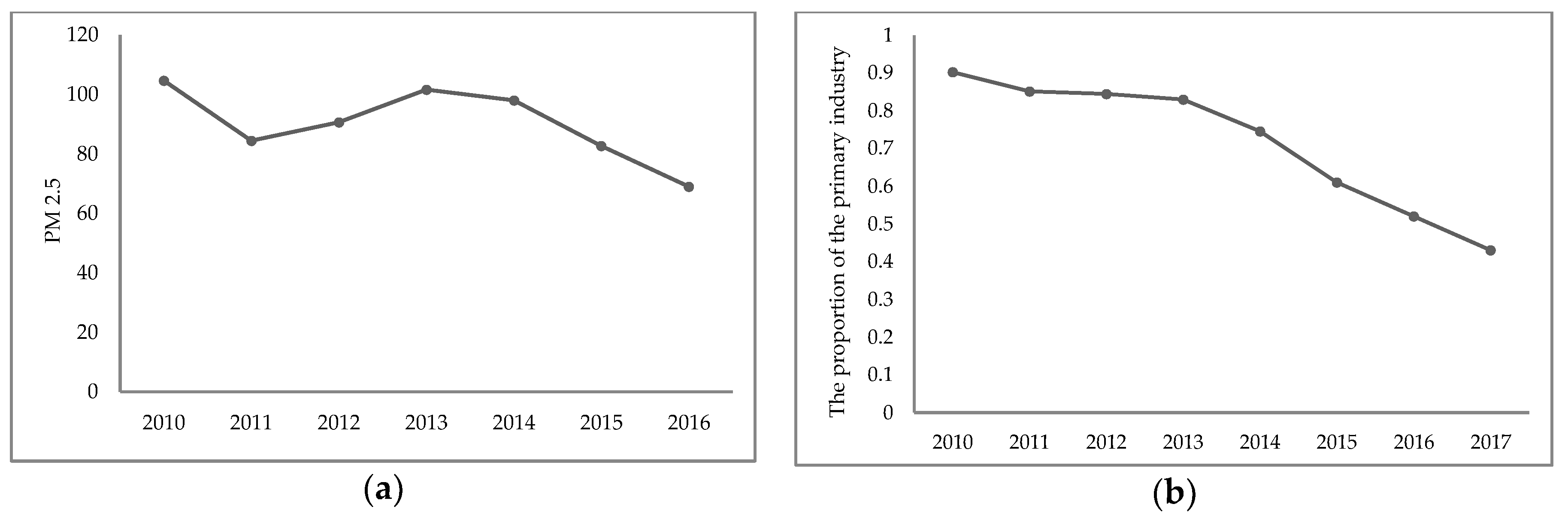
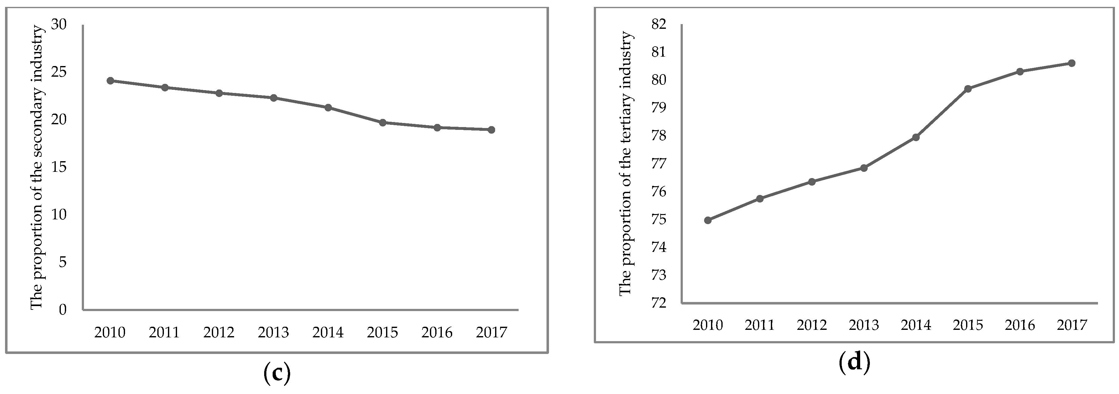
3.2. PM2.5 and the Trends of the Three Industries
3.3. Data Test
3.4. Establishing the VAR Model
3.5. Checking the Model
3.6. Impulse Response Function
3.6.1. Dynamic Relationship between PM2.5 Pollution and the Development of Primary Industry
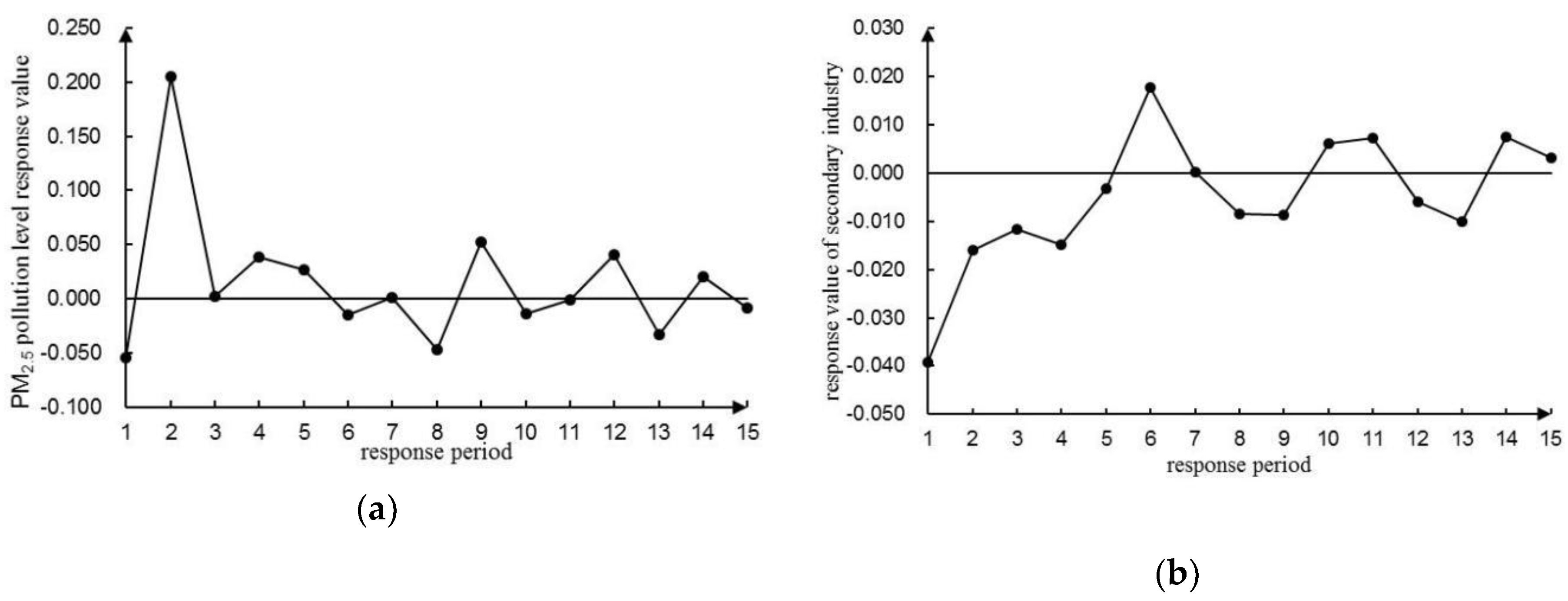
3.6.2. Dynamic Relationship between PM2.5 Pollution Level and the Development of Secondary Industry
3.6.3. Dynamic Relationship between PM2.5 Pollution and the Development of Tertiary Industry
3.7. Variance Decomposition
4. Discussion
5. Conclusions
Author Contributions
Funding
Acknowledgments
Conflicts of Interest
References
- Pollution ‘Worst on Record’ in Beijing. Published on 13 January 2013. Available online: https://www.cnbc.com/id/100375537 (accessed on 21 March 2019).
- Su, D.S. Industry Economics; Higher Education Press: Beijing, China, 2000; pp. 473–474. [Google Scholar]
- Tertiary Sector of the Economy. Available online: https://en.wikipedia.org/wiki/Tertiary_sector_of_the_economy (accessed on 21 March 2019).
- Tipayarom, D.; Oanh, N.T.K. Effects from open rice straw burning emission on air quality in the Bangkok Metropolitan Region. ScienceAsia 2007, 33, 339–345. [Google Scholar] [CrossRef]
- Yan, W.L.; Liu, R.Y.; Sun, Y.; Wei, J.S.; Pu, M.J. Analysis of Continuous Haze and Haze Weather in Jiangsu Province Caused by Straw Incineration. Clim. Environ. Res. 2014, 19, 237–247. [Google Scholar]
- Wu, W.N.; Zha, Y.; Wang, Q.; He, J.L.; Bao, Q. Comparative analysis of winter and summer heavy atmospheric pollution events around Nanjing. China Environ. Sci. 2014, 34, 581–587. [Google Scholar]
- Zhang, L.; Liu, Y.; Hao, L. Contributions of open crop straw burning emissions to PM2.5 concentrations in China. Environ. Res. Lett. 2016, 11, 014014. [Google Scholar] [CrossRef]
- Zhao, T.L.; Liu, D.; Li, T.; Huang, J.P.; Xu, X.D.; Zhou, C.H.; Tang, L.L.; Liu, S.D. Progress of Study on Atmospheric Pollutant Emissions from Agricultural Activity and Their Effect on Atmospheric Environment. Sci. Technol. Eng. 2016, 16, 144–152. [Google Scholar]
- Chameides, W.L.; Yu, H.; Liu, S.C.; Bergin, M.; Zhou, X.; Mearns, L.; Wang, G.; Kiang, C.S.; Saylor, R.D.; Luo, C.; et al. Case study of the effects of atmospheric aerosols and regional haze on agriculture: An opportunity to enhance crop yields in china through emission controls? Proc. Natl. Acad. Sci. USA 1999, 96, 13626–13633. [Google Scholar] [CrossRef]
- Zhang, Y.M. The Influence of Air Pollution in China on Agricultural Environment and Estimation of Economic Loss Costs. Environ. Sci. 1986, 86, 79, 82–86. [Google Scholar]
- Thompson, J.R.; Mueller, P.W.; Flückiger, W.; Rutter, A.J. The effect of dust on photosynthesis and its significance for roadside plants. Environ. Pollut. (Ser. A) 1984, 34, 171–190. [Google Scholar] [CrossRef]
- Farmer, A.M. The effects of dust on vegetation—A review. Environ. Pollut. 1993, 79, 63–75. [Google Scholar] [CrossRef]
- Wen, D.Z.; Kong, G.H.; Zhang, D.Q.; Peng, C.L.; Zhang, R.F.; Li, X. Ecophysiological Responses of 30 gardens plant species exposed to short-term air pollution. Acta Phytoecol. Sin. 2003, 27, 311–317. [Google Scholar]
- Ma, C.C. Hg harm on cell membrane of rape leaf and cell endogenous protection effect. Chin. J. Appl. Ecol. 1998, 9, 323–326. [Google Scholar]
- Cho, U.H.; Park, J.O. Mercury-induced oxidative stress in tomato seedlings. Plant Sci. 2000, 156, 1–9. [Google Scholar] [CrossRef]
- Patra, M.; Sharma, A. Mercury toxicity in plants. Bot. Rev. 2000, 66, 379–422. [Google Scholar] [CrossRef]
- Godbold, D.L.; Hüttermann, A. The uptake and toxicity of mercury and lead to spruce (picea abies karst.) seedlings. Water Air Soil Pollut. 1986, 31, 509–515. [Google Scholar] [CrossRef]
- Zeng, X.F.; Wang, T.Q.; Li, Y. Economic loss of air pollution in Xi’an City. J. Arid Land Resour. Environ. 2015, 29, 105–110. [Google Scholar]
- Chen, J.H.; Bo, Y.Y.; Li, P.S.; Xu, L.W. Study on Characteristics of Air Pollutant Discharge From Industrial Pollution Sources of Beijing City. Ind. Saf. Environ. Prot. 2003, 29, 3–5. [Google Scholar]
- Ehrlich, C.; Noll, G.; Kalkoff, W.D.; Baumbach, G. PM10, PM2.5 and PM1.0—Emissions from industrial plants—results from measurement programmes in Germany. Atmos. Environ. 2007, 41, 6236–6254. [Google Scholar] [CrossRef]
- Leng, Y.L.; Du, S.Z. Industry Structure, Urbanization and Haze Pollution: An Empirical Analysis Based on the Panel Data of Province Level. Forum Sci. Technol. China 2015, 49–55. [Google Scholar]
- Wu, Z.; Zhang, X.; Wu, M. Mitigating construction dust pollution: State of the art and the way forward. J. Clean. Prod. 2016, 112, 1658–1666. [Google Scholar] [CrossRef]
- Xue, Y.F.; Zhou, Z.; Huang, Y.H.; Wang, K. Fugitive Dust Emission Characteristics from Building Construction Sites of Beijing. Environ. Sci. 2017, 38, 2231–2237. [Google Scholar]
- Zhao, Q.; Du, Z.Y.; Hu, J.; Chen, C.C.; Jiang, X.J.; Li, L. Air pollution characteristics and emission sources in Langfang City. Acta Sci. Circumstantiae 2017, 37, 436–445. [Google Scholar]
- Zhou, J. The Main Problems and Development Trends of Industrial Economic Operation. Macroecon. Manag. 2014, 5, 13–16. [Google Scholar]
- Zhang, B.B.; Tian, X.; Zhu, J. Environmental Pollution Control, Marketization and Energy Efficiency: A Theoretical and Empirical Analysis. Soc. Sci. Nanjing 2017. [Google Scholar] [CrossRef]
- He, S.B.; Tan, Q.; Zhou, H.R. Calculating the Reverse Effect of Pollution Reduction on Industrial Structure: An Input-Output Perspective. Stat. Inf. Forum 2015, 30, 15–23. [Google Scholar]
- Cookson, A.H. Electrical breakdown for uniform fields in compressed gases. Proc. Inst. Electr. Eng. 1970, 117, 269–280. [Google Scholar] [CrossRef]
- Tardiveau, P.; Marode, E.; Agneray, A. Tracking an individual streamer branch among others in a pulsed induced discharge. J. Phys. D Appl. Phys. 2002, 35, 2823–2829. [Google Scholar] [CrossRef]
- Xia, L.M.; Zong, H.H. Application of cluster analysis and grey related degree to affecting factors analysis of construction accident. J. Saf. Sci. Technol. 2011, 7, 157–162. [Google Scholar]
- Gong, S.J.; Gao, C.L.; He, G.H. Design of Ventilation and Dust Removal Program for Mechanized Cleaning in Tunnels. Railw. Eng. 2015. [Google Scholar] [CrossRef]
- Zhang, L.H.; Degejirifu; Liang, H.Y. Study on Construction Dust Emission Fee System Levying in China. Environ. Eng. 2016, 34, 74–77. [Google Scholar]
- Rabl, A. Air pollution and buildings: An estimation of damage costs in France. Environ. Impact Assess. Rev. 1999, 19, 361–385. [Google Scholar] [CrossRef]
- Li, X.Y.; Chen, G.C.; Ji, F.Y.; Wang, F.; Zhou, X.J.; Wu, L.P. Estimation of Exposed Stock of Building Materials and Air Pollution-Caused Economic Losses in the Main Urban Area of Chongqing. J. Southwest Univ. (Nat. Sci. Ed.) 2010, 32, 94–99. [Google Scholar]
- Huang, Z.H.; Tang, D.G. Estimation of Vehicle Toxic Air Pollutant Emissions in China. Res. Environ. Sci. 2008, 21, 166–170. [Google Scholar]
- Hara, K.; Homma, J.; Tamura, K.; Inoue, M.; Karita, K.; Yano, E. Decreasing trends of suspended particulate matter and PM2.5 concentrations in Tokyo, 1990–2010. J. Air Waste Manag. Assoc. 2013, 63, 737–748. [Google Scholar] [CrossRef]
- Xu, W.J.; Li, H.X.; Huang, J.Z.; Chen, X.M.; Liu, Y.H. Characteristics of PM2.5 Emission of Vehicles in Foshan City. Environ. Sci. Technol. 2014, 37, 152–158. [Google Scholar]
- Othman, M.; Latif, M.T.; Mohamed, A.F. The PM10, compositions, sources and health risks assessment in mechanically ventilated office buildings in an urban environment. Air Qual. Atmos. Health 2016, 9, 597–612. [Google Scholar] [CrossRef]
- Wang, Y.; Yang, D. Impacts of Freight Transport on PM2.5 Concentrations in China: A Spatial Dynamic Panel Analysis. Sustainability 2018, 10, 2865. [Google Scholar] [CrossRef]
- Wang, R.J.; Wang, K.; Zhang, F.; Gao, J. Emission Characteristics of Vehicles from National Roads and Provincial Roads in China. Environ. Sci. 2017, 38, 3553–3560. [Google Scholar]
- Yang, H.W.; Wan, Y.; Toshihiko, M. The Assessment of Health Impact of Air Pollution on China’s National Economy by Applying a Computable General Equilibrium Model. J. Environ. Health 2005, 22, 166–170. [Google Scholar]
- Kasmo, M.A. The Southeast Asian haze crisis: Lesson to be learned. In Ecosystems and Sustainable Development IV; Tiezzi, E., Brebbia, C.A., Usó, J.L., Eds.; WIT Press: Southampton, UK, 2003; pp. 1263–1271. [Google Scholar]
- Mcnulty, R.P. The effect of air pollutants on visibility in fog and haze at New York city. Atmos. Environ. 1968, 2, 625–628. [Google Scholar] [CrossRef]
- Sajjad, F.; Noreen, U.; Zaman, K. Climate change and air pollution jointly creating nightmare for tourism industry. Environ. Sci. Pollut. Res. 2014, 21, 12403–12418. [Google Scholar] [CrossRef] [PubMed]
- Mu, Q.; Zhang, S.Q. An evaluation of the economic loss due to the heavy haze during January 2013 in China. China Environ. Sci. 2013, 33, 2087–2094. [Google Scholar]
- Cheng, D.N.; Zhou, Y.B.; Wei, X.D.; Wu, J. A Study on the Environmental Risk Perceptions of Inbound Tourists for China Using Negative IPA Assessment. Tour. Trib. 2015, 30, 54–62. [Google Scholar]
- Tang, C.C.; Liu, X.Q.; Song, C.Y. Impact of Haze on Regional Tourism Industry and Its Countermeasures. Geogr. Geo-Inf. Sci. 2016, 32, 121–126. [Google Scholar]
- Liu, K.; Liu, X.Z.; Chang, W.J. An empirical study on the interactions of economic growth and environmental pollution in Yantai—Based on the unrestricted VAR method. Acta Sci. Circumst. 2007, 27, 1929–1936. [Google Scholar]
- Li, M. Research on Economic Growth and Environmental Problems Based on Panel Data. Stat. Decis. 2007, 74–76. [Google Scholar] [CrossRef]
- Xiao, Q.; Gao, Y.; Hu, D.; Tan, H.; Wang, T. Assessment of the Interactions between Economic Growth and Industrial Wastewater Discharges Using Co-integration Analysis: A Case Study for China’s Hunan Province. Int. J. Environ. Res. Public Health 2011, 8, 2937–2950. [Google Scholar] [CrossRef]
- Li, G.; Lei, Y.; Ge, J.; Wu, S. The Empirical Relationship between Mining Industry Development and Environmental Pollution in China. Int. J. Environ. Res. Public Health 2017, 14, 254. [Google Scholar] [CrossRef] [PubMed]
- Duan, X.M.; Guo, J.D. Relationship between Economic Growth and Environmental Pollution in Zhejiang An Empirical Analysis Based on VAR Model. J. Chongqing Jiao Tong Univ. (Soc. Sci. Ed.) 2012, 12, 52–55. [Google Scholar]
- Sims, C.A. Macroeconomics and reality. Econometrica 1980, 48, 1–48. [Google Scholar] [CrossRef]
- Misund, B.; Oglend, A. Supply and demand determinants of natural gas price volatility in the U.K.: A vector autoregression approach. Energy 2016, 111, 178–189. [Google Scholar] [CrossRef]
- Bazzano, A.N.; Oberhelman, R.A.; Potts, K.S.; Gordon, A.; Var, C. Environmental Factors and WASH Practices in the Perinatal Period in Cambodia: Implications for Newborn Health. Int. J. Environ. Res. Public Health 2015, 12, 2392–2410. [Google Scholar] [CrossRef] [PubMed]
- Engle, R.F.; Granger, C.W.J. Co-integration and error correction: Representation, estimation, and testing. Econometrica 1987, 55, 251–276. [Google Scholar] [CrossRef]
- Johansen, S. Statistical analysis of cointegration vectors. J. Econ. Dyn. Control 1988, 12, 231–254. [Google Scholar] [CrossRef]
- Johansen, S.; Juselius, K. Maximum likelihood estimation and inferences on cointegration-with applications to the demand for money. Oxf. Bull. Econ. Stat. 1990, 52, 169–210. [Google Scholar] [CrossRef]
- Granger, C.W.J. Investigating causal relations by econometric models and cross-spectral methods. Econometrica 1969, 37, 424–438. [Google Scholar] [CrossRef]
- Breitung, J.; Brüggemann, R.; Lüetkepohl, H. Structural vector autoregressive modeling and impulse responses. In Applied Time Series Econometrics; Lüetkepohl, H., Kräetzig, M., Eds.; Cambridge University Press: New York, NY, USA, 2004; pp. 159–196. [Google Scholar]
- Beijing Air Pollution: Real-Time Air Quality Index (AQI). Available online: http://aqicn.org/city/beijing/, (accessed on 21 March 2019).
- Liang, X.; Zou, T.; Guo, B.; Li, S.; Zhang, H.; Zhang, S.; Huang, H.; Chen, S.X. Assessing Beijing’s PM2.5 pollution: Severity, weather impact, APEC and winter heating. Proc. R. Soc. A 2015, 471, 20150257. [Google Scholar] [CrossRef]
- Beijing Municipal Bureau of Statistics. Available online: http://tjj.beijing.gov.cn/English/ (accessed on 21 March 2019).
- Shin, K.I. A Multivariate Unit Root Test Based on the Modified Weighted Symmetric Estimator for VAR(p). J. Appl. Stat. 2004, 31, 587–596. [Google Scholar] [CrossRef]
- Koop, G.; Pesaran, M.H.; Potter, S.M. Impulse response analysis in nonlinear multivariate models. J. Econom. 1996, 74, 119–147. [Google Scholar] [CrossRef]
- Pesaran, M.H.; Shin, Y. Generalized impulse response analysis in linear multivariate models. Econ. Lett. 1998, 58, 17–29. [Google Scholar] [CrossRef]
- Cao, L.J. An Empirical Study on the Relationship between Urban Haze and Industrial Structure—Based on Dynamic Panel Model GMM Estimation. J. Huaibei Prof. Tech. Coll. 2016, 15, 79–82. [Google Scholar]
- Zhao, H.; Guo, S.; Zhao, H. Characterizing the Influences of Economic Development, Energy Consumption, Urbanization, Industrialization, and Vehicles Amount on PM2.5 Concentrations of China. Sustainability 2018, 10, 2574. [Google Scholar] [CrossRef]
- Li, L.; Zhu, J.S.; Gao, R.X. The Study on Relationship between Economic Growth and Environmental Pollution in Chongqing Base on VAR Model. J. Southwest Univ. (Nat. Sci. Ed.) 2009, 31, 92–96. [Google Scholar]


| Variables | Stable Seasonality Test | Moving Seasonality Test | ||
|---|---|---|---|---|
| F statistics | Conclusion | F statistics | Conclusion | |
| RPM | 1.271 | no evidence of stable seasonality | 0.600 | no evidence of moving seasonality |
| RPI | 1.258 | no evidence of stable seasonality | 1.321 | no evidence of moving seasonality |
| RSI | 6.197 | no evidence of stable seasonality | 1.070 | no evidence of moving seasonality |
| RTI | 0.060 | no evidence of stable seasonality | 0.771 | no evidence of moving seasonality |
| Variables | Test Form | ADF Statistics | Stationarity | Trend Item | Intercept | Lag Order | Conclusion |
|---|---|---|---|---|---|---|---|
| RPM | (C,T,K) | −5.786205 | stationary ** | none | none | 0 | stationary without intercept item and trend item |
| (C,0,K) | −5.671215 | stationary ** | — | none | 0 | ||
| (0,0,K) | −5.292310 | stationary ** | — | — | 0 | ||
| RPI | (C,T,K) | −4.835591 | stationary ** | existence ** | existence ** | 0 | stationary with trend item |
| (C,0,K) | — | — | — | — | — | ||
| (0,0,K) | — | — | — | — | — | ||
| RSI | (C,T,K) | −3.960725 | stationary ** | none | existence * | 0 | stationary with intercept item |
| (C,0,K) | −3.804746 | stationary ** | — | existence ** | — | ||
| (0,0,K) | — | — | — | — | — | ||
| RTI | (C,T,K) | −5.534724 | stationary ** | none | existence ** | 0 | stationary with intercept item |
| (C,0,K) | −5.426812 | stationary ** | — | existence ** | 0 | ||
| (0,0,K) | — | — | — | — | — |
| Lag | LR | FPE | AIC | SC | HQ |
|---|---|---|---|---|---|
| 0 | NA | 1.52 × 10⁻⁹ | −8.95534 | −8.756966 * | −8.90861 |
| 1 | 29.32872 * | 1.19 × 10⁻⁹ | −9.22601 | −8.23415 | −8.99236 |
| 2 | 10.57243 | 2.69 × 10⁻⁹ | −8.58473 | −6.79939 | −8.16416 |
| 3 | 14.85528 | 3.66 × 10⁻⁹ | −8.78077 | −6.20194 | −8.17328 |
| 4 | 23.30377 | 5.60 × 10⁻¹⁰ * | −11.98698 * | −8.61467 | −11.19256 * |
| Null Hypothesis | Eigenvalue | Trace Test | Maximum Eigenvalue Test | ||
|---|---|---|---|---|---|
| Statistics | 5% Critical Value | Statistics | 5% Critical Value | ||
| no cointegration relationship * | 0.9784 | 151.8784 | 63.8761 | 84.3802 | 32.1183 |
| at most one cointegration relationship * | 0.9225 | 67.4982 | 42.9153 | 56.2640 | 25.8232 |
| at most two cointegration relationships | 0.2896 | 11.2342 | 25.8721 | 7.5235 | 19.3870 |
| Null Hypothesis | χ2 Statistics | p-Value | Conclusion |
|---|---|---|---|
| RPI is not a Granger cause of RPM | 25.55 | 0.000 | refuse * |
| RSI is not a Granger cause of RPM | 37.11 | 0.000 | refuse * |
| RTI is not a Granger cause of RPM | 50.12 | 0.000 | refuse * |
| All are not a Granger cause of RPM | 161.93 | 0.000 | refuse * |
| RPM is not a Granger cause of RPI | 0.94 | 0.919 | accept |
| RPM is not a Granger cause of RSI | 2.76 | 0.599 | accept |
| RPM is not a Granger cause of RTI | 0.80 | 0.938 | accept |
| Time | Contribution Rate of Three Industries to PM2.5 | Contribution Rate of PM2.5 to Three Industries | ||||
|---|---|---|---|---|---|---|
| RPI (%) | RSI (%) | RTI (%) | RPI (%) | RSI (%) | RTI (%) | |
| 1 | 1.4343 | 66.3280 | 6.1932 | 0.0000 | 0.0000 | 0.0000 |
| 2 | 0.5011 | 24.8786 | 72.6510 | 0.2118 | 0.0008 | 0.0296 |
| 3 | 4.8225 | 23.6702 | 69.3508 | 0.1297 | 0.6037 | 0.3569 |
| 4 | 35.3334 | 18.4177 | 44.8152 | 0.1374 | 0.4304 | 0.3506 |
| 5 | 37.3774 | 18.1013 | 43.0945 | 0.1152 | 1.1778 | 0.3353 |
| 6 | 35.7270 | 19.3533 | 43.3784 | 0.1133 | 1.2785 | 0.3639 |
| 7 | 35.7366 | 19.3414 | 43.3107 | 0.1189 | 1.5279 | 0.3737 |
| 8 | 34.3263 | 18.5498 | 45.5829 | 0.1519 | 1.6385 | 0.3723 |
© 2019 by the authors. Licensee MDPI, Basel, Switzerland. This article is an open access article distributed under the terms and conditions of the Creative Commons Attribution (CC BY) license (http://creativecommons.org/licenses/by/4.0/).
Share and Cite
Chen, J.; Chen, K.; Wang, G.; Wu, L.; Liu, X.; Wei, G. PM2.5 Pollution and Inhibitory Effects on Industry Development: A Bidirectional Correlation Effect Mechanism. Int. J. Environ. Res. Public Health 2019, 16, 1159. https://doi.org/10.3390/ijerph16071159
Chen J, Chen K, Wang G, Wu L, Liu X, Wei G. PM2.5 Pollution and Inhibitory Effects on Industry Development: A Bidirectional Correlation Effect Mechanism. International Journal of Environmental Research and Public Health. 2019; 16(7):1159. https://doi.org/10.3390/ijerph16071159
Chicago/Turabian StyleChen, Jibo, Keyao Chen, Guizhi Wang, Lingyan Wu, Xiaodong Liu, and Guo Wei. 2019. "PM2.5 Pollution and Inhibitory Effects on Industry Development: A Bidirectional Correlation Effect Mechanism" International Journal of Environmental Research and Public Health 16, no. 7: 1159. https://doi.org/10.3390/ijerph16071159
APA StyleChen, J., Chen, K., Wang, G., Wu, L., Liu, X., & Wei, G. (2019). PM2.5 Pollution and Inhibitory Effects on Industry Development: A Bidirectional Correlation Effect Mechanism. International Journal of Environmental Research and Public Health, 16(7), 1159. https://doi.org/10.3390/ijerph16071159