Article

Geospatial Distributions of Groundwater Quality in Gedaref State Using Geographic Information System (GIS) and Drinking Water Quality Index (DWQI)

1
Department of Environmental Science and Engineering, Faculty of Geosciences and Environmental Engineering, Southwest Jiaotong University, high-tech zone, Chengdu 611756, China
2
Department of Hydrogeology, Faculty of Petroleum & Minerals, Al Neelain University, Khartoum 11121, Sudan
3
School of Resources and Environment, University of Electronic Science and Technology of China, Chengdu 611756, China
4
Key Laboratory of Digital Earth, Institute of Remote Sensing and Digital Earth, Chinese Academy of Sciences, No. 9 Dengzhuang South Road, Haidian District, Beijing 100094, China
5
Water Environmental Sanitation Project (WES), Gedaref State Water Corporation, Gedaref 32214, Sudan
*
Author to whom correspondence should be addressed.
Int. J. Environ. Res. Public Health 2019, 16(5), 731; https://doi.org/10.3390/ijerph16050731
Submission received: 4 December 2018 / Revised: 14 February 2019 / Accepted: 17 February 2019 / Published: 28 February 2019
(This article belongs to the Section Environmental Science and Engineering)

Abstract

:
The observation of groundwater quality elements is essential for understanding the classification and distribution of drinking water. Geographic Information System (GIS) and remote sensing (RS), are intensive tools for the performance and analysis of spatial datum associated with groundwater sources control. In this study, groundwater quality parameters were observed in three different aquifers including: sandstone, alluvium and basalt. These aquifers are the primary source of national drinking water and partly for agricultural activity in El Faw, El Raha (Fw-Rh), El Qalabat and El Quresha (Qa-Qu) localities in the southern part of Gedaref State in eastern Sudan. The aquifers have been overworked intensively as the main source of indigenous water supply in the study area. The interpolation methods were used to demonstrate the facies pattern and Drinking Water Quality Index (DWQI) of the groundwater in the research area. The GIS interpolation tool was used to obtain the spatial distribution of groundwater quality parameters and DWQI in the area. Forty samples were assembled and investigated for the analysis of major cations and anions. The groundwater in this research is controlled by sodium and bicarbonate ions that defined the composition of the water type to be Na HCO3. However, from the plots of piper diagram; the samples result revealed (40%) Na-Mg-HCO3 and (35%) Na-HCO3 water types. The outcome of the analysis reveals that several groundwater samples have been found to be suitable for drinking purposes in Fa-Rh and Qa-Qu areas.

1. Introduction

Groundwater is a noble resource for water in arid and semiarid areas [1,2,3,4,5,6]. Accessibility to water is an important global goal whose effects are abundantly felt in developing countries. The benefit of understanding groundwater geochemistry is to ensure its good quality for drinking [7,8,9]. In arid and semi-arid areas, the potential use of groundwater for drinking and agricultural projects is threatened by the decline of water quality due to physical and anthropogenic characteristics. Evaluation of the geochemical status of groundwater is required to competently plan and control the groundwater resources [10]. The interaction between water and rocks has usually been studied to provide an understanding of the physical and chemical procedures controlling water chemistry [11,12,13]. Several factors control the groundwater geochemistry such as the type of rock forming the aquifer, the residence time of water in the hosted aquifer, the origin of the groundwater and the flow directions of groundwater [14,15].
The estimation of quality and the use of groundwater for different purposes are becoming more significant [16]. Thus, probes related to an understanding of the hydro-chemical aspects of the groundwater, geochemical processes and its development under natural water flowing manners, not only aids in the practical utilization and protection of this expensive resource but also aid in visualizing the changes in the groundwater environment [17,18].
Statistical analysis methods such as the correlation matrix, bivariate, and Hierarchal component analysis; produce a reliable alternative procedure for understanding and explaining the complex system of water quality with the capability of analyzing large amounts of data [19].
GIS and RS, are intensive tools for performance and analysis of spatial datum associated with groundwater sources control. Remote sensing data are essential in many geo-resources, such as mineral research, hydrogeology, and other geologic fields [20]. It is important in hydrogeological reconnaissance for understanding structural, geomorphological, and lithological features. The acquired RS information improves our knowledge of the hydrogeological conditions. Satellite images are universally applied for qualitative estimation of groundwater resources by investigating geological structures, geomorphic features, and their hydrological characteristics [21,22,23]. The spatial distribution maps were designed and integrated within ArcGIS v.10.5 software.
Drinking water quality index (DWQI) presents a single number to reveal the overall water quality at a particular position and time, based on various water quality factors. It is interpreted as a number that indicates the combined impact of several water quality parameters [19,24,25,26,27,28]. DWQI has been popularly utilized in water quality evaluations for both surface and sub-surface water, and it has represented an increasingly significant function in the water resource environment and management [29,30,31].
Shortage of drinking water in East Central Sudan especially in the basaltic terrain is a common problem. Most of the rural community depends on groundwater sources in their daily life for drinking purposes. This research aims to generate groundwater distribution maps and to evaluate water quality for drinking purposes in Qa-Qu and Fw-Rh areas in the southern part of Gedaref State in eastern Sudan. The area consists of one of the essential agricultural fields of Gedaref State, the El Rahad project which was developed as a mechanized project in Sudan in 1978 [32].
In this work, forty samples were observed and monitored from selected boreholes. Hence, an attempt of statistical analysis methods such as correlation matrix and Hierarchal component analysis were applied to determine the variation in hydro-chemical facies and understand the development of hydro-chemical processes. Moreover, adopting Piper and Durov diagrams by use of Aqua Chem. v.2014.2 software, to classify the groundwater facies and water types in the area. The world health organization (WHO) [33] standard has been used for correlations with the results of sample analysis to examine the permissible amount of water for drinking.
The analytical results achieved from the samples when plotted on Piper’s plot, explained that the alkalis (Na+, K+), appear considerably over the alkaline elements (Ca2+, Mg2+), and the weak acidic (HCO3) appear considerably over strong acidic anions (Cl & SO4−2). Moreover, the Piper diagram matched 40% of the samples, under Na-Mg-HCO3 group and 35% under Na-HCO3 type. According to the plotting from the Durov diagram, most of the elements of water plotted within the HCO3·Na zone, except some other samples that fell in HCO3 Cl-Na, SO4·Cl·HCO3-Na, or HCO3·Cl-Na·Mg types. DWQI was calculated by adopting weighted arithmetical index methods considering thirteen water quality parameters (pH, TDS, Ca+2, Mg+2, Na+, K+, Fe+2, Cl, HCO3, SO4−2, F, NO3, and E.C) in order to assess the degree of groundwater contamination and suitability for drinking purposes.
For the better understanding of geological units in this project, the thin sections of rock samples have been generated. With this ability, the rock mineral contents have been determined much better. This study has great importance; due to the plan for obtaining drinking water from the groundwater sources to Fw-Rh and Qa-Qu localities. However, this investigation is helpful in understanding groundwater environments and its suitability for human uses, especially in arid and semi-arid regions.

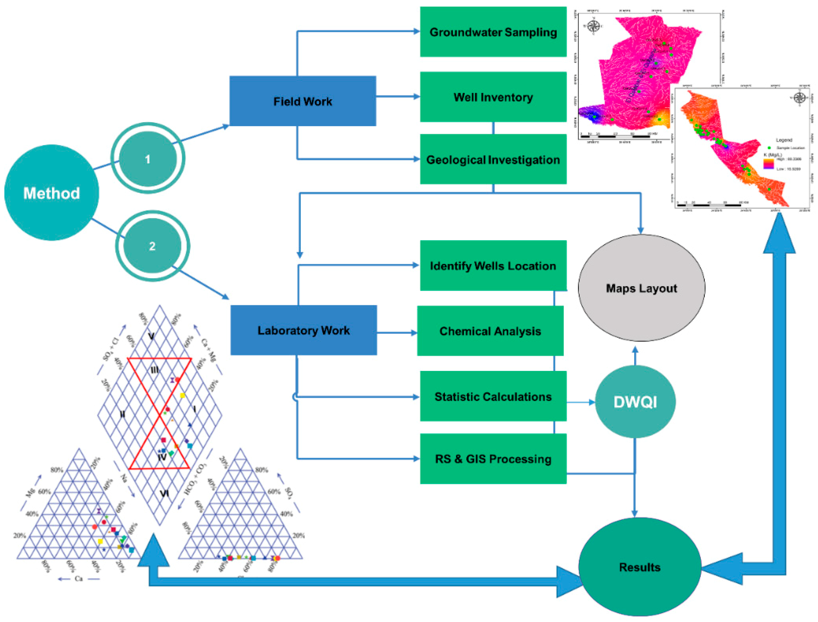
2. Materials and Methods
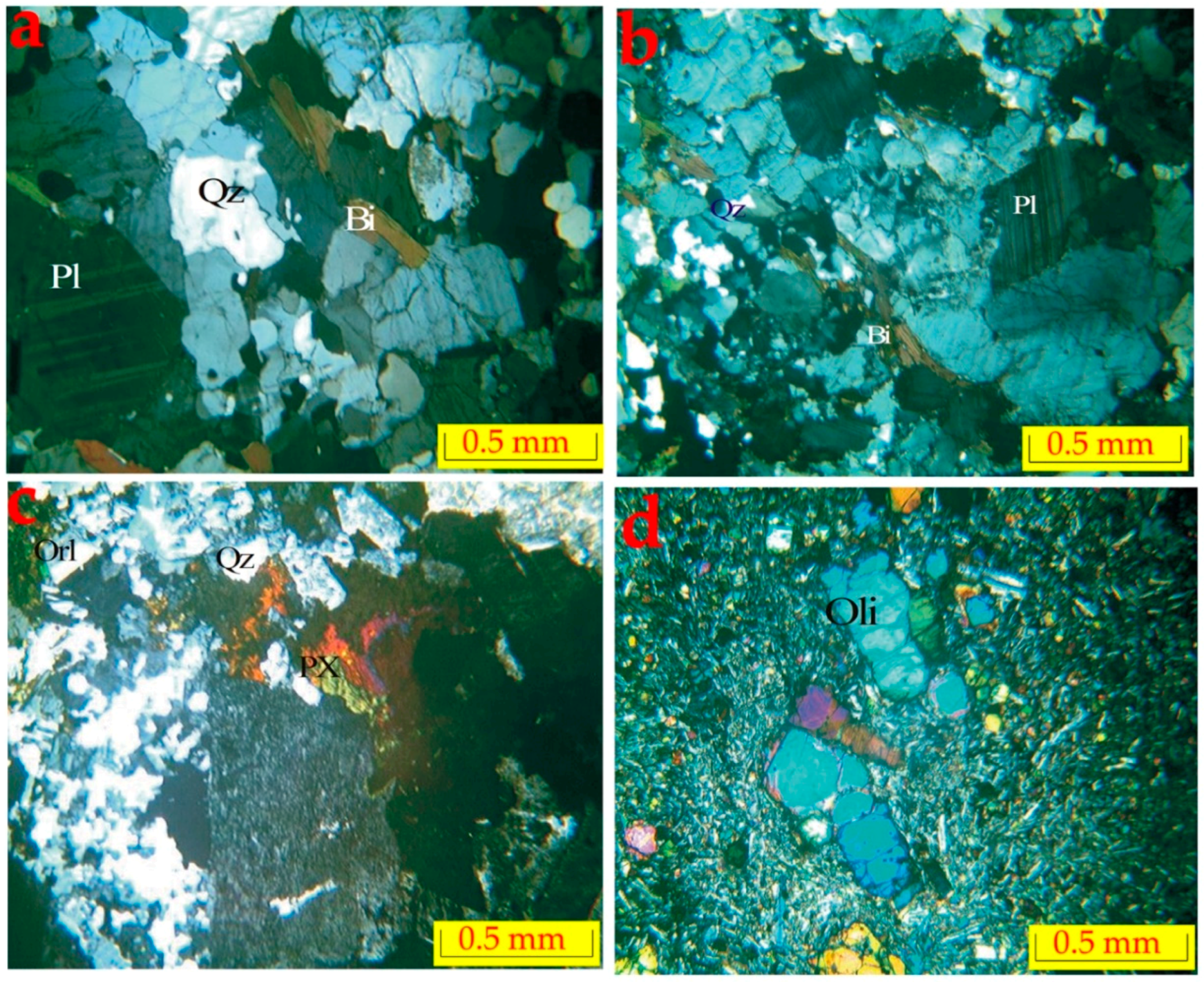
2.1. Geology

Geologically Figure 1; the lower Proterozoic rocks of the basement complex (Mainly Granitic Gneisses) [34], Syn-orogenic Granit and Syn-orogenic gabbro underlain the sandstone of Gedaref formation, Tertiary (Oligocene) basalt [35], Umm Rawaba formation, sand sheets and recent alluvium and wadi deposits. The groundwater of the area was taped at the sandstone of Gedaref formation sequence, alluvium soil, and fractures of the Oligocene basalt aquifers with depths ranging from 14 to 64 m.

2.2. Hydrogeological Setting

The groundwater was studied by using the data collected from forty boreholes drilled in Fw-Rh and Qa-Qu area as seen in Table 1. The hydrogeological characteristics of rock units were investigated, and aquifer systems were determined depending on field investigations and previous studies. Therefore, the hydrogeological map of the Fw-Rh and Qa-Qu area was settled adopting ArcGIS v.10.5 software, based on characteristics of the lithological units Figure 2. According to these evaluations, the aquifer types were described as sandstone, alluvium, and fracture basalt.

2.3. Spatial Interpolation and Groundwater Quality Mapping

Spatial interpolation is a procedure of predicting the value of attributes at unsampled sites from measurements made at point locations within the same area [36]. There are two main groupings of interpolation techniques: deterministic and geostatistical. Deterministic interpolation techniques create surfaces from measured points, based on either the extent of similarity (e.g., Inverse Distance Weighted) or the degree of smoothing (e.g., radial basis functions). Geostatistical interpolation techniques (e.g., kriging) utilize the statistical properties of the measured points.
In this study, we found that the Kriging (Ordinary and Simple) interpolation method is the most suitable method. Thus, the histograms and normal QQplots were plotted to examine the normality distribution of the observed data for each water quality element in both Fw-Rh and Qa-Qu localities.

2.4. Drinking Water Quality Index DWQI

DWQI has been determined based on the standards of drinking water quality as counseled by WHO. Therefore, thirteen chemical parameters (pH, TDS, Ca, Mg, Na, K, Cl, HCO3, F, NO3, Fe, and E.C.) were used for the calculation. To apply DWQI in the current study, the study area was divided into two parts, Fw-Rh, and Qa-Qu localities. The water quality parts were generated by a weighting factor and then formerly aggregated by using the simple mean calculations. To estimate the water quality in this project, the quality rating (Qi) for all elements was estimated through the following equation;
Q i = { ( V a V i / V s V i ) } 100
where, Qi = Quality ranking of the element form a total number of water quality elements, Va = Real amount of the water quality element taken from laboratory study, Vi = Ideal rate of the water quality element can be realized from the standard Tables. Vi for pH = 7 and for other elements it is equaling to zero. Vs standard = Value of WHO standard.
Then, the Relative weight (Wr) was studied from inversed proportional of recommended standard (Si) for the corresponding parameter using the following expression;
W r = I S i
Here Wr = Relative (unit) weight for specific element; Si = Standard allowable amount for certain element; I = Proportionality constant.
Assuredly, the total DWQI was determined using the assemblage equations of the quality rating with the unit weight linearly as the following:
DWQI =   Q i W r /   W r #
where Qi = Quality rating; Wr = Relative weight.
In general, DWQI is determined for particular and intended uses of water. In this work, the DWQI was estimated for human consumption, and the maximum DWQI value for the drinking purposes was regarded as 100 scores.
The methodology ideas in this work have been done through several steps Figure 3.

3. Results

Several factors may control the groundwater geochemistry such as the type of rock forming the aquifer, residence time of water in the hosted aquifer, the origin of the groundwater and the flow directions of groundwater. Hydro-chemical properties of the groundwater of the area are shown in Table 2. The water pH ranges between 7.5 and 8.9, indicate an alkaline chemical reaction in both sandstone and basaltic aquifers. The electrical conductivity (E.C) varies from 345 to 3342 μS/cm.

3.1. Interpolation and Elements Distribution Maps

The quality of interpolation is described by the difference of the interpolated value from the true value. Thus, the Anderson-Darling test, which is an ECDF (empirical cumulative distribution function) based test, tests the prospect that the value of a parameter falls within a particular range of values (confidence level 95%). The data points are relatively close to the fitted normal distribution line. The p-value is greater than the significance level of 0.05. Subsequently, the scientist fails to reject the null hypothesis that the data follow a normal distribution.
According to this test, in Fw-Rh area we found that the parameters (Na and K) showed a normal distribution when the other elements (Ca, Mg, HCO3, Cl, SO4 and TDS) showed a more or less abnormal distribution in Figure 4 and Figure 5.
The same test has been performed in (Qa-Qu) area, which showed that the (Mg and SO4) parameters reflected normal distribution while the other variables (Ca, K, Na, HCO3, Cl, and TDS) present non-normally distributions.
Generally, most of the collected elements in both Fw-Rh and Qa-Qu localities were skewed. However, the transformations (Log & BoxCox), have been used to make the data normally distributed and satisfy the assumption of equal variability for the data.
For the maps prediction, several kinds of semivariogram models were examined for each water quality parameter to obtain the preferable one, as seen in Figure 6 as an example. Predictive performances of the fitted models were checked on the basis of cross-validation tests. The values of mean error (ME), mean square error (MSE), root mean error (RMSE), average standard error (ASR) and root mean square standardized error (RMSSE) were estimated to ascertain the performance of the developed models. After conducting the cross-validation procedure, maps of kriged estimates were created that provided a visual representation of the distribution of the groundwater quality parameters in the Fw-Rh and Qa-Gu areas.
Kriging (Ordinary and Simple) interpolation method is the most suitable method in the studied areas. The value range of the better interpolation models were observed and reported in Table 3. If the RMSE is close to the ASE, the prediction errors were assessed correctly. If the RMSE is smaller than the ASE, then the variability of the predictions is overestimated; conversely, if the RMSE is greater than the ASE, then the variability of the predictions is underestimated. The same could be deduced from the RMSSE statistic. It should be close to one. If the RMSSE is greater than one, the variability of the predictions is underestimated; also, if it is minimal than one, the variability is overestimated. After generating the cross-validation procedure, estimated maps of kriging were created, which gives a visual representation of the distribution of the groundwater quality parameters.
The hydro-chemical of Fw-Rh area; the sodium concentration patterns in Figure 7a show similar trends to the potassium in Figure 7b with higher values in the northwest and southeast when decreasing in the central part. The distribution of calcium Figure 7c, ranges from 4.54 mg/L to 37.47 mg/L, it reflects relatively moderate values in the middle of Fw-Rh area. The distribution of magnesium Figure 7d, ranges from 11.66 mg/L to 34.28 mg/L. It also reflects the relatively moderate value in the middle of the area. The bicarbonate HCO3 concentration Figure 7e, varies from 78.9 mg/L to 1450.00 mg/L, when the concentration of chloride Figure 7f, ranges from 8.10 mg/L to mg/L 172.50. The distribution of sulfate Figure 7g, ranges from 0.02 to 2.57, with a similar orientation as the TDS Figure 7h, both appear with higher values at the central part, moderate values in the southeast and low values in the northwest. The Fw-Ra consists most of the acidic rocks and Alluvium soil with clay layers in the project area, (i.e., granitic intrusions), thus, the origin of its most elements could be from weathering, hydro-chemical reactions and the solubility of minerals (i.e., The existence of potassium and sodium associated to the kaolin’s rich alunite (K, Na)Al3(SO4)2(OH)6] [36]); (Thirteen thematic layers of water quality parameters were used in ArcGIS environment to acquire the output of drinking water quality index DWQI maps for Fw-Rh Figure 8a, and Qa-Qu Figure 8b, localities. The water quality index was reclassified into five classes in order to characterize the quality of groundwater in the studied localities.
The hydro-chemical of Qa-Qu area; the sodium concentration in Figure 9a has similar trends as the potassium Figure 9b, with higher values in the east, middle values in the northwest to the north and low values in the southern part. The distribution of calcium in Figure 9c, ranges from 10.44 mg/L to 53.00 mg/L, the high values concentrated in the middle of Qa-Qu area, then decreases gradually to the north and south. The magnesium Figure 9d, ranges from 11.56 mg/L to 72.00 mg/L. It reflects random distribution values in the Qa-Qu area. The bicarbonate HCO3 concentration Figure 9e, varies from 118.60 mg/L to 930.00 mg/L, when the concentration of chloride in Figure 9f, ranges from 10.00 mg/L to mg/L 45.00. The distribution of sulfate in Figure 9g, ranges from 1.36 to 2.29, with the highest values in the southeast and lowest values in the southwest. The TDS in Figure 9h, ranges from 183.00 mg/L to 2007.00 mg/L, appears with low to medium values at the central part then, increases to the southeasterly direction. The Qa-Qa area represented the most of Gedaref Formation, which is superimposed and intercalated by basaltic rocks (Oligocene) and substantially covered by the clay soils. Thus, the origin of most of its cations could be from chemical weathering, hydro-chemical reactions and the solubility of minerals (See thirteen thematic layers of water quality parameters used in ArcGIS environment to acquire the output of drinking water quality index DWQI maps for Fw-Rh Figure 10a, and Qa-Qu Figure 10b, localities. The water quality index was reclassified into five classes in order to characterize the quality of groundwater in the studied localities.

3.2. Correlation Matrix

The correlation matrix provides the assessment of the correlation coefficients “r” between groundwater quality elements. These coefficients are applied to suppress the strength of the linear relationship between the variables. It has been used to estimate both positive and negative correlations. The project area describes three examples of groundwater aquifers; (1) sandstone aquifer, dominant at Fw-Rh area; (11 Boreholes) and subdominant at Qa-Qu area; (5 Boreholes). (2) Alluvium aquifer, dominant at Fw-Rh area; (12 Boreholes) and only one borehole at Qa-Qu area. (3) Basaltic aquifer found as (five boreholes) at Qa-Qu area. (Table 4); Fw-Rh; reveal a strong positive correlation can be identified between Na+/K+ (r = 0.99), TDS/E.C (r = 0.99), E.C/Mg+2 (r = 0.55), TDS/Mg+2 (r = 0.53), and Ca+2/K+ (r = 0.51). It is found that NO3 in most of the groundwater samples in this locality reflected strong correlations as: NO3/TDS (r = 0.56), NO3/E.C (r = 0.55), and NO3/Ca+2 (r = 0.50).
(Qa-Qu); the magnesium has a strong positive correlation between most of the groundwater elements; Mg+2/Ca+2 (r = 0.75), Mg+2/SO4−2 (r = 0.73), Mg+2/HCO3 (r = 0.54), Mg+2/K+ (r = 0.41), and Mg+2/Na+ (r = 0.40). Another positive correlation can be identified very strongly between; Na+/K+ (r = 0.99), HCO3/SO4−2 (r = 0.70), NO3/Fe+2 (r = 0.66), and pH/HCO3 (r = 0.57). The strong negative correlation in (Qa-Qu) area, indicated as: Mg+2/NO3 (r = −0.54), Cl/Fe+2 (r = −0.46) pH/Na+ (r = −0.38), Mg+2/K+, (r = −0.38), and Ca+2/F (r = −0.35) (Table 5).

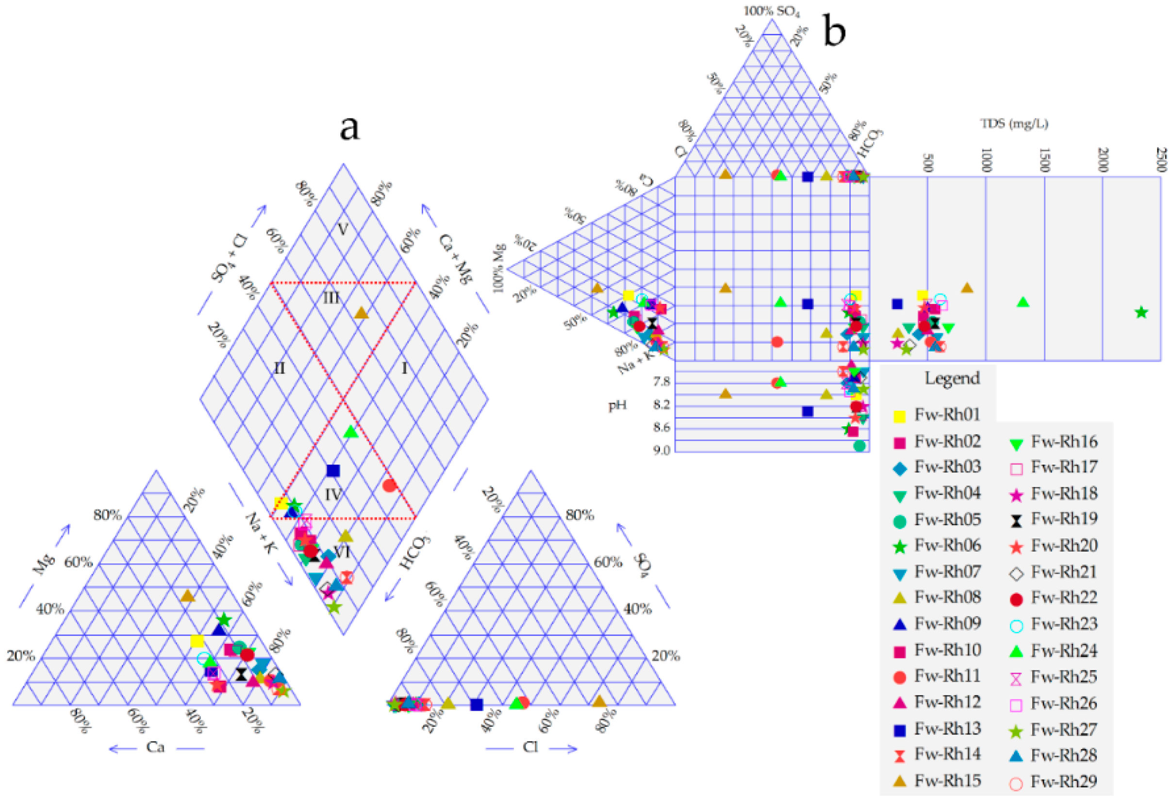
3.3. Groundwater Facies

Groundwater facies were defined by applying a Piper plot and Durov diagrams as seen in Figure 11 and Figure 12. The descriptions reveal that the area consists of eight groups of groundwater types Table 6, Na-Mg-HCO3, Na-HCO3, Na-Ca-HCO3, Na-Ca-Mg-HCO3, Mg-Na-Ca-Cl, Mg-Na-HCO3, Na-Ca-Mg-HCO3-Cl, and Na-Mg-Ca-HCO3. The analytical results achieved from the samples when plotted on Piper’s plot, explained that the alkalis (Na+, K+), appear considerably over the alkaline elements (Ca+2, Mg+2), and the weak acidic (HCO3) appear considerably over strong acidic anions (Cl & SO4−2). Moreover, Piper diagram matched 40% of the samples, under Na-Mg-HCO3 group and 35% under Na-HCO3 type.
According to the plotting from the Durov diagram, most of the elements of water plotted within the HCO3·Na zone, except some other samples that were fell in HCO3 Cl–Na, SO4·Cl·HCO3–Na, or HCO3·Cl–Na·Mg types.

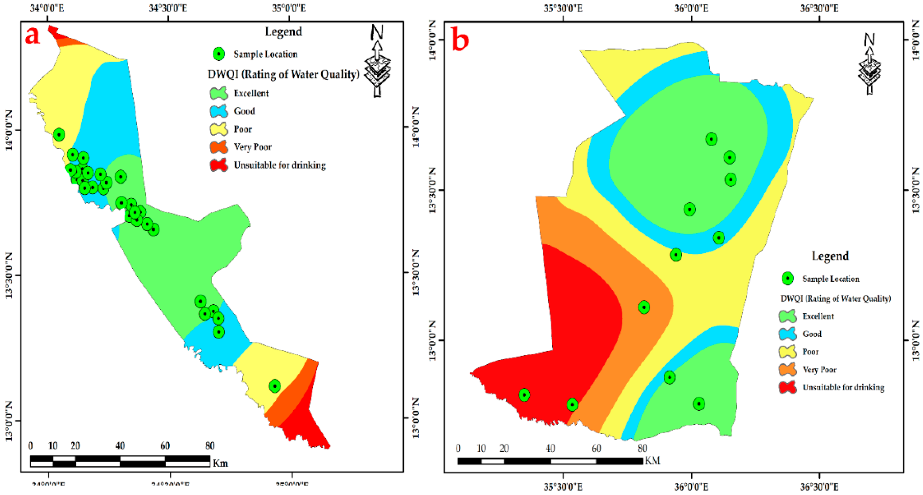
3.4. Drinking Water Quality Index (DWQI)

To gain a comprehensive representation of the quality of the drinking groundwater, drinking water quality index (DWQI) is one of the useful tools. It supplies a single amount to a state’s overall water quality at a specific location and time, based on a number of water quality parameters. DWQI in Table 7, was calculated by adopting weighted arithmetical index method considering thirteen water quality parameters (pH, TDS, Ca+2, Mg+2, Na+, K+, Fe+2, Cl, HCO3, SO4−2, F, NO3, and E.C) in order to assess the degree of groundwater contamination and suitability.
Thirteen thematic layers of water quality parameters were used in the ArcGIS environment to acquire the output of drinking water quality index DWQI maps for Fw-Rh Figure 13a, and Qa-Qu Figure 13b, localities. The water quality index was reclassified into five classes in order to characterize the quality of groundwater in the studied localities.

4. Discussion

In this study, most of the boreholes were recently drilled (2015–2017), no other boreholes were available. Due to the few observation points, limited previous investigations and few hydrogeological data, using geospatial distributions, GIS and DWQI provide support in groundwater studies. As far as we know, no other study was conducted using the techniques in Fw-Rh and Qa-Qu areas.
The chemical composition and elements concentration of groundwater, are related to the rocks lithology and time residence of the water in the aquifers. To identify the effects of the reaction between the groundwater and the (geological units) aquifer, the bivariate diagrams were applied to explain the chemical changes in ionic concentrations in the host rocks and groundwater. The reaction between water and the surrounding surface/soil from agricultural fields can change groundwater chemistry. The bivariate diagram of NO3 vs. TDS and E.C, Figure 14a,b, records that six samples of alluvium aquifer and two samples of sandstone aquifer, plots along the 1:1 aquiline, show the highest correlation among TDS/NO3. The appearance of NO3 associated with the fertilizers activities in the agricultural farms [37,38,39]. The elements Na+ versus K+ Figure 14c, at both sandstone and alluvium aquifers, reflects a linear relationship at (r = 0.99) suggesting the reactions of water with sodium feldspar (Albite) and potassium feldspar (Orthoclase) in equations five and six respectively. The Mg+2 strongly correlated with Ca+2 and SO4−2 Figure 14d,e, especially in the basaltic aquifer and some other boreholes in the alluvium locations, show a high response of water with a group of minerals (i.e., Pyroxene, Olivine and Biotite) in equations seven, eight, and nine respectively. For the better understanding of geological units in research areas, the thin sections of rock samples have been generated and studied to identify the main mineral composition for each rock sample, as seen in Figure 15. With this ability, the rock mineral contents have been determined much better.
The main mechanism for the dissolution of rock minerals that releases the element such as: (Ca, Mg, Na, K and HCO3); into the groundwater, have been indicated in the following reactions:
( Pl ) Anorthite :   CaAl 2 Si 2 O 3 + 2 CO 3 + H 2 O     Al 2 Si 2 O 5 ( OH ) 4 + Ca 2 + + 2 HCO 3
( Pl ) Albite : 2 NaAl 3 O 8 + 9 H 2 O + 2 H +   Al 2 Si 2 O 5 ( OH ) 4 + 4 H 4 SiO 4 + 2 Na +
( Orl )   Orthoclase : 2 KAlSi 3 O 8 + 11 H 2 O   Si 2 O 5 Al 2 ( OH ) 4 + 2 K + + 2 OH
( Px ) Pyroxene :   CaMg ( Si 2 O 6 ) + 4 CO 2 + 6 H 2 O   Ca 2 + + Mg 2 +   4 HCO 3 + 2 Si ( OH ) 4
( Oli ) Olivine ( Fe , Mg 2 + ) S i O 4 + 4 H 2 CO 3   2 ( Fe , Mg 2 + ) + H 4 Si O 4 + 4 HCO 3
( Bi )   Biotite :   K ( Mg ,   Fe ) 3 ( AlSi 3 O 10 ) ( F , OH 2 ) + 5 H 2 O + 4 CO 2 )   K + Mg + Fe ( OH ) 3 + 4 HCO 3 + H + 2 F

5. Conclusions

This study explains the geospatial distribution, adopting statistical methods with GIS to characteristics and mapped the groundwater quality in the different hydrogeological units such as sandstone, alluvium, and basaltic aquifers, which are located in eastern Sudan (the southwestern part of Gedaref State). Forty water boreholes samples from different locations were collected, analyzed and estimated.
Aqua Chem v.2014.2 software has been used for groundwater quality elements analysis, while ArcGIS software was chosen for the interpretation and spatial mapping, so that groundwater quality estimation studies have been completed successfully. This study envisions the significance of graphical illustrations, i.e., Piper, Bivariate, Dendrogram, and Durov diagrams plot, to determine variation in hydro-chemical facies and to understand the evolution of hydro-chemical processes in Qa-Qu and Fw-Rh areas.
The hydrogeochemical evaluation outcomes and distribution of groundwater cations (Na+, Ca+2, K+, Mg+2) and anions (HCO3, Cl, SO4−2, F) in both the Qa-Qu and Fw-Rh areas, shows that the groundwater is chemically affected by aquifer lithology. According to the plotting from the Durov diagram, most of the elements of water plotted within the HCO3·Na zone, except some other samples that fell in HCO3 Cl–Na, SO4·Cl·HCO3–Na, or HCO3·Cl–Na Mg types. With the exclusion of a few elements, the quality of groundwater is mostly suitable for drinking purposes and other domestic uses. The groundwater in this project is controlled by sodium and bicarbonate ions, which define the composition of the water type to be Na HCO3. According to this investigation, three potential aquifers (sandstone, alluvium, and basalt); have been identified in the research areas.
The DWQI was used to determine the groundwater quality and its suitability for drinking purposes. According to this investigation, 20% of groundwater samples represent “excellent water”, 50% indicate “good water”, 15% represent “poor water”, 7.5% shows “very poor water”, and 7.5% appear as “unsuitable for drinking”. The drinking water quality index that was produced for this study reveals that the northwest and southeast parts of Fw-Rh and the southwest part of Qa-Qu locations has the poorest water quality, which is classified as “unsuitable for drinking”.
It should be noted, that the actual variations in spatial interpolations, can considerably diverge from the values predicted by spatial interpolation, it may lead to probable limitations of Kriging especially when data is scarce and unequally distributed. Thus, it is essential to know the number of data locations and the geographical extent of the region containing those data locations. In this case, one of the crucial steps is estimating the variogram model, which is more difficult with a small number of data locations. In this study, the transformations (Log & BoxCox), have been used to make the data normally distributed and satisfy the assumption of equal variability for the data. Several types of semivariogram models were tested in Table 3, for all water quality parameters to achieve more reliable results.

Author Contributions

T.H., B.A.E. & J.Z. had the initial idea for the research project and writing of the article, M.M.B., W.A. & B.A.E. accomplished fieldwork, data acquisition and implemented the research experiments, K.M.E. & E.H.A. helping in data analysis and maps layout, H.T. supervise the plan and evaluate the conclusion of the manuscript.

Funding

This study financially supported by the Sichuan Environmental Engineering Assessment Center Project Technical Consultation on Comprehensive Assessment of Groundwater Pollution Status in Typical Industrial Park of Shiyang, Deyang (2017H01013).

Acknowledgments

The authors thank the Water Corporation of Gedaref State—Sudan (WCGSS) and Water Environmental Sanitation (WES), Project Gedaref State—Sudan; for the technical support of this study.

Conflicts of Interest

The authors declare no conflict of interest.

References

  1. Li, P.; Wu, J.; Tian, R.; He, S.; He, X.; Xue, C.; Zhang, K. Geochemistry, hydraulic connectivity and quality appraisal of multilayered groundwater in the Hongdunzi coal mine, northwest China. Mine Water Environ. 2018, 37, 222–237. [Google Scholar] [CrossRef]
  2. Ferchichi, H.; Hamouda, M.B.; Farhat, B.; Mammou, A.B. Assessment of groundwater salinity using GIS and multivariate statistics in a coastal Mediterranean aquifer. Int. J. Environ. Sci. Technol. 2018, 15, 2473–2492. [Google Scholar] [CrossRef]
  3. Tiwari, A.K.; Ghione, R.; De Maio, M.; Lavy, M. Evaluation of hydrogeochemical processes and groundwater quality for suitability of drinking and irrigation purposes: A case study in the Aosta Valley region, Italy. Arabian J. Geosci. 2017, 10, 264. [Google Scholar] [CrossRef]
  4. Kura, N.U.; Ramli, M.F.; Sulaiman, W.N.A.; Ibrahim, S.; Aris, A.Z.; Mustapha, A. Evaluation of factors influencing the groundwater chemistry in a small tropical island of Malaysia. Int. J. Environ. Res. Public Health 2013, 10, 1861–1881. [Google Scholar] [CrossRef] [PubMed]
  5. Bhusari, V.; Katpatal, Y.; Kundal, P. Performance evaluation of a reverse-gradient artificial recharge system in basalt aquifers of Maharashtra, India. Hydrogeol. J. 2017, 25, 689–706. [Google Scholar] [CrossRef]
  6. Vesali Naseh, M.R.; Noori, R.; Berndtsson, R.; Adamowski, J.; Sadatipour, E. Groundwater Pollution Sources Apportionment in the Ghaen Plain, Iran. Int. J. Environ. Res. Public Health 2018, 15, 172. [Google Scholar] [CrossRef] [PubMed]
  7. Appelo, C.A.J.; Postma, D. Geochemistry, Groundwater and Pollution; CRC Press: Amsterdam, The Netherlands, 2004; p. 647. [Google Scholar]
  8. Chacha, N.; Njau, K.N.; Lugomela, G.V.; Muzuka, A.N. Hydrogeochemical characteristics and spatial distribution of groundwater quality in Arusha well fields, Northern Tanzania. Appl. Water Sci. 2018, 8, 118. [Google Scholar] [CrossRef]
  9. Nelly, K.C.; Mutua, F. Ground Water Quality Assessment Using GIS and Remote Sensing: A Case Study of Juja Location, Kenya. Am. J. Geogr. Inf. Syst. 2016, 5, 12–23. [Google Scholar]
  10. Ravikumar, P.; Somashekar, R. Principal component analysis and hydrochemical facies characterization to evaluate groundwater quality in Varahi river basin, Karnataka state, India. Appl. Water Sci. 2017, 7, 745–755. [Google Scholar] [CrossRef]
  11. Varol, S.; Davraz, A. Evaluation of the groundwater quality with WQI (Water Quality Index) and multivariate analysis: A case study of the Tefenni plain (Burdur/Turkey). Environ. Earth Sci. 2015, 73, 1725–1744. [Google Scholar] [CrossRef]
  12. Eang, K.E.; Igarashi, T.; Kondo, M.; Nakatani, T.; Tabelin, C.B.; Fujinaga, R. Groundwater monitoring of an open-pit limestone quarry: Water-rock interaction and mixing estimation within the rock layers by geochemical and statistical analyses. Int. J. Min. Sci. Technol. 2018, 28, 849–857. [Google Scholar] [CrossRef]
  13. Ahmed, A.; Clark, I. Groundwater flow and geochemical evolution in the Central Flinders Ranges, South Australia. Sci. Total Environ. 2016, 572, 837–851. [Google Scholar] [CrossRef] [PubMed]
  14. Tóth, J. Groundwater as a geologic agent: An overview of the causes, processes, and manifestations. Hydrogeol. J. 1999, 7, 1–14. [Google Scholar] [CrossRef]
  15. Zaki, S.R.; Redwan, M.; Masoud, A.M.; Moneim, A.A.A. Chemical characteristics and assessment of groundwater quality in Halayieb area, southeastern part of the Eastern Desert, Egypt. Geosci. J. 2018, 23, 149–164. [Google Scholar] [CrossRef]
  16. Gidey, A. Geospatial distribution modeling and determining suitability of groundwater quality for irrigation purpose using geospatial methods and water quality index (WQI) in Northern Ethiopia. Appl. Water Sci. 2018, 8, 82. [Google Scholar] [CrossRef]
  17. Lawrence, A.; Gooddy, D.; Kanatharana, P.; Meesilp, W.; Ramnarong, V. Groundwater evolution beneath Hat Yai, a rapidly developing city in Thailand. Hydrogeol. J. 2000, 8, 564–575. [Google Scholar] [Green Version]
  18. Edmunds, W.; Ma, J.; Aeschbach-Hertig, W.; Kipfer, R.; Darbyshire, D. Groundwater recharge history and hydrogeochemical evolution in the Minqin Basin, North West China. Appl. Geochem. 2006, 21, 2148–2170. [Google Scholar] [CrossRef]
  19. Castilla-Hernández, P.; del Rocío Torres-Alvarado, M.; Herrera-San Luis, J.A.; Cruz-López, N. Water quality of a reservoir and its major tributary located in east-central Mexico. Int. J. Environ. Res. Public Health 2014, 11, 6119–6135. [Google Scholar] [CrossRef] [PubMed]
  20. Pande, C.B.; Moharir, K. Spatial analysis of groundwater quality mapping in hard rock area in the Akola and Buldhana districts of Maharashtra, India. Appl. Water Sci. 2018, 8, 106. [Google Scholar] [CrossRef]
  21. Das, S.; Behera, S.; Kar, A.; Narendra, P.; Guha, S. Hydrogeomorphological mapping in ground water exploration using remotely sensed data—A case study in keonjhar district, orissa. J. Indian Soc. Remote Sens. 1997, 25, 247–259. [Google Scholar] [CrossRef]
  22. Abdalla, F. Mapping of groundwater prospective zones using remote sensing and GIS techniques: A case study from the Central Eastern Desert, Egypt. J. Afr. Earth Sci. 2012, 70, 8–17. [Google Scholar] [CrossRef]
  23. Moubark, K.; Abdelkareem, M. Characterization and assessment of groundwater resources using hydrogeochemical analysis, GIS, and field data in southern Wadi Qena, Egypt. Arabian J. Geosci. 2018, 11, 598. [Google Scholar] [CrossRef]
  24. Şener, Ş.; Şener, E.; Davraz, A. Evaluation of water quality using water quality index (WQI) method and GIS in Aksu River (SW-Turkey). Sci. Total Environ. 2017, 584, 131–144. [Google Scholar] [CrossRef] [PubMed]
  25. Sahu, P.; Sikdar, P.J.E.G. Hydrochemical framework of the aquifer in and around East Kolkata Wetlands, West Bengal, India. Environ. Geol. 2008, 55, 823–835. [Google Scholar] [CrossRef]
  26. Rubio-Arias, H.; Contreras-Caraveo, M.; Quintana, R.M.; Saucedo-Teran, R.A.; Pinales-Munguia, A. An overall water quality index (WQI) for a man-made aquatic reservoir in Mexico. Int. J. Environ. Res. Public Health 2012, 9, 1687–1698. [Google Scholar] [CrossRef] [PubMed]
  27. De La Mora-Orozco, C.; Flores-Lopez, H.; Rubio-Arias, H.; Chavez-Duran, A.; Ochoa-Rivero, J. Developing a water quality index (WQI) for an irrigation dam. Int. J. Environ. Res. Public Health 2017, 14, 439. [Google Scholar] [CrossRef] [PubMed]
  28. Iqbal, M.; Shoaib, M.; Farid, H.; Lee, J. Assessment of Water Quality Profile Using Numerical Modeling Approach in Major Climate Classes of Asia. Int. J. Environ. Res. Public Health 2018, 15, 2258. [Google Scholar] [CrossRef] [PubMed]
  29. Ravikumar, P.; Somashekar, R.; Prakash, K. A comparative study on usage of Durov and Piper diagrams to interpret hydrochemical processes in groundwater from SRLIS river basin, Karnataka, India. Elixir Earth Sci. 2015, 80, 31073–31077. [Google Scholar]
  30. Wu, Z.; Wang, X.; Chen, Y.; Cai, Y.; Deng, J. Assessing river water quality using water quality index in Lake Taihu Basin, China. Sci. Total Environ. 2018, 612, 914–922. [Google Scholar] [CrossRef] [PubMed]
  31. Misaghi, F.; Delgosha, F.; Razzaghmanesh, M.; Myers, B. Introducing a water quality index for assessing water for irrigation purposes: A case study of the Ghezel Ozan River. Sci. Total Environ. 2017, 589, 107–116. [Google Scholar] [CrossRef] [PubMed]
  32. Tameim, O.; Zakaria, Z.; Hussein, H.; el Gaddal, A.A.; Jobin, W.R. Control of schistosomiasis in the new Rahad Irrigation Scheme of Central Sudan. J. Trop. Med. Hyg. 1985, 88, 115–124. [Google Scholar] [PubMed]
  33. World Health Organization. Guidelines for drinking-water quality: First addendum to the fourth edition; World Health Organization: Geneva, Switzerland, 2017; p. 631. [Google Scholar]
  34. Ibrahim, K.; Hussein, M.; Giddo, I. Application of combined geophysical and hydrogeological techniques to groundwater exploration: A case study of Showak-Wad Elhelew area, Eastern Sudan. J. Afr. Earth Sci. 1992, 15, 1–10. [Google Scholar] [CrossRef]
  35. Eisawi, A.; Schrank, E. Terrestrial palynology and age assessment of the Gedaref Formation (eastern Sudan). J. Afr. Earth Sci. 2009, 54, 22–30. [Google Scholar] [CrossRef]
  36. Wipki, M.; Germann, K.; Schwarz, T. Alunitic kaolins of the Gedaref region (NE-Sudan). In Geoscientific Research in Northeast Africa; CRC Press: Berlin, Germany, 2017; pp. 509–514. [Google Scholar]
  37. Dawelbeit, M.I.; Babiker, E.J.S. Effect of tillage and method of sowing on wheat yield in irrigated Vertisols of Rahad, Sudan. Soil Tillage Res. 1997, 42, 127–132. [Google Scholar] [CrossRef]
  38. Saunders, D.A. Wheat in Heat-stressed Environments: Irrigated, Dry Areas, and Rice-wheat Farming Systems: Proceedings of the International Conferences: Wheat in Hot, Dry, Irrigated Environments, Wad Medani, Sudan, 1-4 February 1993, Wheat in Warm Area, Rice-wheat Farming Systems, Dinajpur, Bangladesh, 13-15 Feburary [sic] 1993; CIMMYT: Wad Medani, Sudan, 1994; p. 415. [Google Scholar]
  39. Mozafar, A. Nitrogen fertilizers and the amount of vitamins in plants: A review. J. Plant Nutr. 1993, 16, 2479–2506. [Google Scholar] [CrossRef]
Figure 1. Location map and geological units of study area.
Ijerph 16 00731 g001
Figure 2. Hydrogeological map of the study area.
Ijerph 16 00731 g002
Figure 3. Methodology chart of study procedures.
Ijerph 16 00731 g003
Figure 4. Graphical summary and probability plots of cations in Fw-Rh area.
Ijerph 16 00731 g004
Figure 5. Graphical summary and probability plots of HCO3, SO4−2, Cl & TDS in Fw-Rh area.
Ijerph 16 00731 g005
Figure 6. An example of Cross Validation Comparison. (a) Ordinary Kriging Spherical and (b) ordinary Kriging-Circular for Na element.
Ijerph 16 00731 g006
Figure 7. (a) Na, (b) K, (c) Ca, (d) Mg, (e) HCO3, (f) SO4, (g) Cl and, (h) TDS distributions in Fw-Rh area.
Ijerph 16 00731 g007
Figure 8. Spatial interpolation of Drinking Water Quality Index (DWQI). (a) Fw-Rh and (b) Qa-Qu localities Discussion.
Ijerph 16 00731 g008
Figure 9. (a) Na, (b) K, (c) Ca, (d) Mg, (e) HCO3, (f) SO4, (g) Cl, and, (h) TDS distributions in Qa-Qu area.
Ijerph 16 00731 g009
Figure 10. Spatial interpolation of Drinking Water Quality Index (DWQI). (a) Fw-Rh and (b) Qa-Qu localities discussion.
Ijerph 16 00731 g010
Figure 11. (a) Piper and (b) Durov diagrams of Fw-Rh area.
Ijerph 16 00731 g011
Figure 12. (a) Piper and (b) Durov diagrams of Qa-Qu area.
Ijerph 16 00731 g012
Figure 13. Spatial interpolation of DWQI, (a) Fw-Rh and (b) Qa-Qu localities.
Ijerph 16 00731 g013
Figure 14. Bivariate diagrams of ionic relations in groundwater of different aquifers.
Ijerph 16 00731 g014
Figure 15. Selective rock thin sections: (a) Granite, (b) Migmatite gneiss, (c) Quartz Syenite, and Oligocene basalt (Qtz = quartz, Pl = plagioclase, Bi = Biotite, Orl = orthoclase, Px = pyroxene, & Oli = olivine).
Ijerph 16 00731 g015
Table 1. Hydrogeological data of forty wells drilled in the study area.
Aquifer TypeWell Depth (m)S.W.L (M)Elevation (m)Water Table (m)Well Name
Alluvium2316425409Ellewatah3
Sandstone2716424408Abu Kalbo
Sandstone6437423386Um Rakuba
Sandstone4827425398Um Tireaza
Sandstone2111444432Um Tireaza 2
Sandstone6013554505Macancana
Sandstone4811.94426414Wd Margi
Sandstone2111446435Mohamed Ali
Alluvium 147424417Um Gazaz
Sandstone6412425413Wad Elkarar1
Alluvium 2719424405Eldar Elbeida
Sandstone4213655634Ellewatah2
Alluvium 2716486470Halaly5
Alluvium 3014427413Wad Elwosta
Alluvium 5734424383Wad Elkarar2
Basaltic4224423410Hilat Ali
Alluvium 22.512428416Abu Saeed
Alluvium 2813427414Elyas
Alluvium 2612648634Elmeageerah
Sandstone257598591Dora
Well CodeAquifer TypeWell Depth (m)S.W.L (M)Elevation (m)Water Table (m)
Fw-Rh21Alluvium 3414447433
Fw-Rh22Alluvium 1810444434
Fw-Rh23Alluvium 5741433399
Fw-Rh24Alluvium 2618428410
Fw-Rh25Alluvium 2114422411
Fw-Rh26Basaltic158658650
Fw-Rh27Alluvium 2410428418
Fw-Rh28Alluvium 218431423
Fw-Rh29Alluvium 2316425409
Qa-Qu01Sandstone5332627595
Qa-Qu02Sandstone6049426413
Qa-Qu03Alluvium 2112422411
Qa-Qu04Basaltic4221631607
Qa-Qu05Basaltic2614454442
Qa-Qu06Sandstone4335500465
Qa-Qu07Alluvium 2716428412
Qa-Qu08Sandstone2111431417
Qa-Qu09Sandstone5742635593
Qa-Qu10Sandstone3121447426
Qa-Qu11Basaltic309650641
Table 2. Descriptive statistical analysis result of water samples (N = 40).
Fw-Rh (N = 29)Qa-Qu (N = 11)
VariableWHOMinimumMaximumMeanStd. D.MinimumMaximumMeanStd. D.
pH7.0–8.07.508.908.030.357.608.707.960.32
TDS (mg/L)1000242.002340.00601.72399.60183.002007.00663.18502.41
Ca754.45130.0037.4730.0610.4453.0022.2112.43
Mg3011.66120.5334.2823.8611.5672.0036.2018.23
Na20076.00359.00214.2869.8776.00597.00167.18150.29
K-15.0070.0041.7213.4016.00115.0033.3628.68
Cl2508.10172.5035.9037.6910.0045.0021.398.96
HCO3-78.901450.00499.35311.78118.60930.00355.40247.40
SO42500.022.570.740.701.362.291.830.31
F0.5–10.012.560.550.550.022.560.650.70
NO3500.2015.003.883.961.5011.105.053.11
Fe0.030.010.800.150.220.011.040.190.31
E.C (µ.S/cm)-345.003342.00888.23570.54281.539692.001777.972721.19
(WHO)= The world health organization standard.
Table 3. Characteristics parameters of variogram models.
AreaGroundwater ParametersKriging TypeTransformationBest Fitted ModelMERMSEASEMSERMSSE
Fw-RhNaSimpleNoneSpherical−1.598571.005173.1880−0.02260.9816
KOrdinaryNoneSpherical−0.281813.610814.0445−0.02070.9817
CaOrdinaryLogCircular0.657932.148630.10620.01551.0624
MgOrdinaryLogGaussian0.521018.985322.6372−0.02240.8808
HCO3OrdinaryBoxCoxStable19.5080328.5189367.53600.04980.9083
ClOrdinaryLogCircular−0.415138.029937.4075−0.00771.0432
SO4OrdinaryBoxCoxStable0.05930.66930.63510.08921.0814
TDSOrdinaryBoxCoxStable12.4257434.6693453.43100.02941.0040
Qa-QuNaSimpleNoneStable10.9458143.4509156.62270.06880.8907
KSimpleLogSpherical−0.168327.114219.2757−0.01021.4215
CaSimpleBoxCoxStable−0.376114.104211.5697−0.01761.1645
MgOrdinaryLogCircular1.659320.618023.8640−0.06151.0218
HCO3OrdinaryBoxCoxStable15.3778261.7170258.98170.05560.9939
ClOrdinaryLogStable−0.37369.63357.1223−0.11651.2648
SO4OrdinaryNoneSpherical0.02510.32090.31930.06541.0026
TDSSimpleBoxCoxGaussian6.7649614.1923453.6139−0.28291.8464
(ME)= Values of mean error, (RMSE)= Root mean error, (ASE)= Average standard error, (MSE)= Mean square error, (RMSSE)= Root mean square standardized error.
Table 4. Correlation matrix analysis result of the groundwater quality parameters in Fw-Rh area.
VariablespHTDSCaMgNaKClHCO3SO4FNO3FeE.C
pH1
TDS0.201
Ca0.110.261
Mg0.100.530.311
Na−0.300.020.230.071
K−0.310.020.230.080.991
Cl−0.140.330.510.490.130.151
HCO3−0.11−0.16−0.070.10−0.010.00−0.101
SO40.100.05−0.080.01−0.17−0.180.06−0.341
F−0.26−0.17−0.35−0.210.140.13−0.180.09−0.261
NO30.250.560.490.320.240.240.16−0.190.03−0.211
Fe−0.15−0.14−0.15−0.41−0.02−0.02−0.09−0.26−0.170.13−0.061
E.C0.190.990.240.550.000.000.34−0.160.05−0.160.55−0.151
Values in bold are different from 0 with a significance level alpha = 0.5.
Table 5. Correlation matrix analysis result of the groundwater quality parameters in Qa-Qu area.
VariablespHTDSCaMgNaKClHCO3SO4FNO3FeE.C
pH1
TDS0.091
Ca0.150.051
Mg0.13−0.090.751
Na−0.38−0.090.040.401
K−0.38−0.090.040.410.991
Cl0.330.450.290.06−0.19−0.191
HCO30.57−0.210.520.540.000.01−0.071
SO40.24−0.160.370.730.430.44−0.150.701
F−0.27−0.22−0.35−0.18−0.09−0.09−0.16−0.42−0.301
NO3−0.260.06−0.19−0.54−0.15−0.15−0.34−0.08−0.50−0.161
Fe0.18−0.16−0.05−0.26−0.29−0.29−0.460.08−0.27−0.110.661
E.C−0.130.24−0.16−0.040.140.160.130.170.34−0.270.15−0.231
Values in bold are different from 0 with a significance level alpha = 0.5.
Table 6. Groundwater facies distribution in the study area.
Water TypeFw-RhQa-QuWater Type %
Na-Mg-HCO310616 (40%)
Na-HCO311314 (35%)
Na-Ca-Mg-HCO3303 (7.5%)
Na-Ca-HCO3303 (7.5%)
Mg-Na-Ca-Cl101 (2.5%)
Mg-Na-HCO3011 (2.5%)
Na-Ca-Mg-HCO3-Cl101 (2.5%)
Na-Mg-Ca-HCO3011 (2.5%)
Table 7. DWQI for groundwater samples in (Fw-Rh-Qa-Qu) area.
DWQI ValueRating of Water QualityPercent %Fw-Rh AreaQa-Qu Area
0–25Excellent8 (20%)53
25–50Good20 (50%)173
51–100Poor6 (15%)33
101–200Very Poor3 (7.5%)21
>>200Unsuitable for drinking3 (7.5%)21

