Associations between Urban Sprawl and Life Expectancy in the United States


Abstract
:1. Introduction
2. Materials and Methods
2.1. Data and Variables
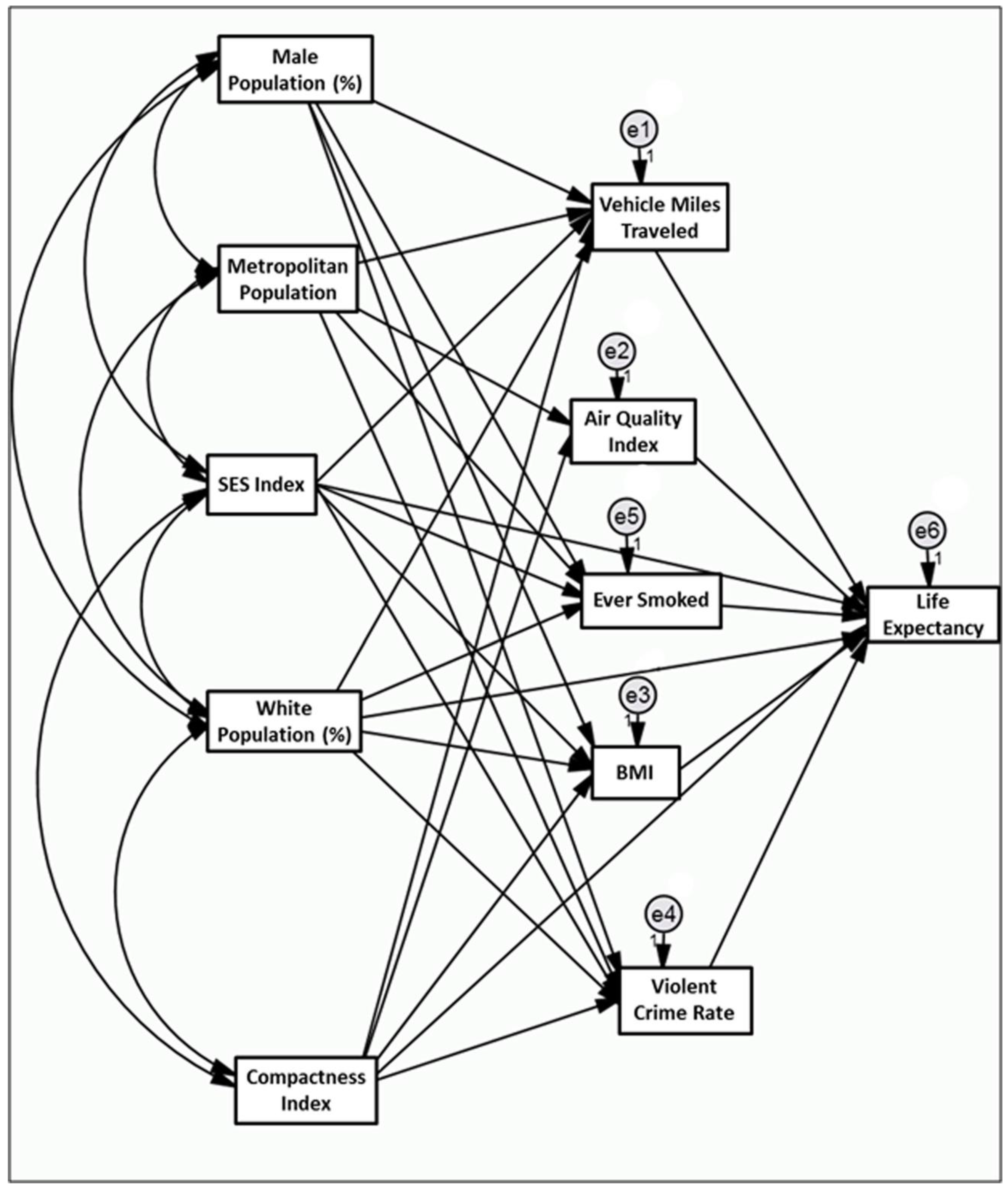
2.2. Statistical Analysis
3. Results
4. Discussion
5. Conclusions
Author Contributions
Acknowledgments
Conflicts of Interest
References
- World Health Organization. World Health Statistic Annual 2013; WHO: Geneva, Switzerland, 2013. [Google Scholar]
- Crimmins, E.M.; Preston, S.H.; Cohen, B. (Eds.) Explaining Divergent Levels of Longevity in High-Income Countries; National Academies Press: Washington, DC, USA, 2011; p. 17. [Google Scholar]
- Kindig, D.A.; Cheng, E.R. Even as mortality fell in most US counties, female mortality nonetheless rose in 42.8 percent of counties from 1992 to 2006. Health Aff. 2013, 32, 451–458. [Google Scholar] [CrossRef] [PubMed]
- Murray, C.J.; Kulkarni, S.C.; Michaud, C.; Tomijima, N.; Bulzacchelli, M.T.; Iandiorio, T.J.; Ezzati, M. Eight Americas: Investigating mortality disparities across races, counties, and race-counties in the United States. PLoS Med. 2006, 3, e260. [Google Scholar]
- Mirowsky, J.; Ross, C. Socioeconomic Status and Subjective Life Expectancy. Soc. Psychol. Q. 2000, 63, 133–151. [Google Scholar] [CrossRef]
- Ezzati, M.; Friedman, A.; Kulkarni, S.; Murray, C. The Reversal of Fortunes: Trends in County Mortality and Cross-County Mortality Disparities in the United States. PLoS Med. 2008, 5, 557–568. [Google Scholar]
- Olshansky, S.J.; Antonucci, T.; Berkman, L.; Binstock, R.H.; Boersch-Supan, A.; Cacioppo, J.T.; Carnes, B.A.; Carstensen, L.L.; Fried, L.P.; Goldman, D.P.; et al. Differences in life expectancy due to race and educational differences are widening, and many may not catch up. Health Aff. 2012, 31, 1803–1813. [Google Scholar] [CrossRef] [PubMed]
- Crimmins, E.M.; Saito, Y. Trends in healthy life expectancy in the United States, 1970–1990: Gender, racial, and educational differences. Soc. Sci. Med. 2001, 52, 1629–1641. [Google Scholar] [CrossRef]
- Olshansky, S.J.; Carnes, B.A.; Désesquelles, A. Demography: Prospects for human longevity. Science 2001, 291, 1491–1492. [Google Scholar] [CrossRef] [PubMed]
- Olshansky, S.J.; Passaro, D.J.; Hershow, R.C.; Layden, J.; Carnes, B.A.; Brody, J.; Hayflick, L.; Butler, R.N.; Allison, D.B.; Ludwig, D.S. A potential decline in life expectancy in the United States in the 21st century. N. Engl. J. Med. 2005, 352, 1138–1145. [Google Scholar] [CrossRef] [PubMed]
- Swanson, D.A.; Sanford, A.G. Socio-Economic Status and Life Expectancy in the United States, 1990–2010: Are We Reaching the Limits of Human Longevity? Popul. Rev. 2012, 51, 16–40. [Google Scholar]
- Mellor, J.M.; Milyo, J. Income inequality and health status in the United States: Evidence from the current population survey. J. Hum. Resour. 2002, 37, 510–539. [Google Scholar] [CrossRef]
- Wilkinson, R.G.; Pickett, K.E. Income inequality and population health: A review and explanation of the evidence. Soc. Sci. Med. 2006, 62, 1768–1784. [Google Scholar] [CrossRef] [PubMed]
- Harper, S.; Lynch, J.; Burris, S.; Smith, G.D. Trends in the black-white life expectancy gap in the United States, 1983–2003. JAMA 2007, 297, 1224–1232. [Google Scholar] [CrossRef] [PubMed]
- Danaei, G.; Rimm, E.; Oza, S.; Kulkarni, S.; Murray, C.; Ezzati, M. The promise of prevention: The effects of four preventable risk factors on national life expectancy and life expectancy disparities by race and county in the United States. PLoS Med. 2010, 7, 1–13. [Google Scholar] [CrossRef] [PubMed]
- Christenson, B.; Johnson, N. Educational Inequality in Adult Mortality: An Assessment with Death Certificate Data from Michigan. Demography 1995, 32, 215–229. [Google Scholar] [CrossRef] [PubMed]
- Elo, I.; Preston, S. Educational Differentials in Morality: United States, 1979–85. Soc. Sci. Med. 1996, 42, 47–57. [Google Scholar] [CrossRef]
- Manton, K.G.; Stallard, E. Health and disability differences among racial and ethnic groups. In National Research Council, Racial and Ethnic Differences in the Health of Older Americans; Martin, L.G., Soldo, B.J., Eds.; Committee on Population. Commission on Behavioral and Social Sciences and Education; National Academy Press: Washington, DC, USA, 1997; pp. 43–104. [Google Scholar]
- Meara, E.R.; Richards, S.; Cutler, D.M. The gap gets bigger: Changes in mortality and life expectancy, by education, 1981–2000. Health Aff. 2008, 27, 350–360. [Google Scholar] [CrossRef] [PubMed]
- US Department of Health and Human Services. The Health Consequences of Smoking: A Report of the Surgeon General; US Department of Health and Human Services, Centers for Disease Control and Prevention, National Center for Chronic Disease Prevention and Health Promotion, Office on Smoking and Health: Atlanta, GA, USA, 2004; Volume 62.
- Stewart, S.T.; Cutler, D.M.; Rosen, A.B. Forecasting the effects of obesity and smoking on US life expectancy. N. Engl. J. Med. 2009, 361, 2252–2260. [Google Scholar] [CrossRef] [PubMed]
- Kaplan, R.M.; Anderson, J.P.; Kaplan, C.M. Modeling quality-adjusted life expectancy loss resulting from tobacco use in the United States. Soc. Indic. Res. 2007, 81, 51–64. [Google Scholar] [CrossRef]
- Streppel, M.T.; Boshuizen, H.C.; Ocké, M.C.; Kok, F.J.; Kromhout, D. Mortality and life expectancy in relation to long-term cigarette, cigar and pipe smoking: The Zutphen Study. Tob. Control 2007, 16, 107–113. [Google Scholar] [CrossRef] [PubMed]
- Mokdad, A.H.; Marks, J.S.; Stroup, D.F.; Gerberding, J.L. Actual causes of death in the United States, 2000. JAMA 2004, 291, 1238–1245. [Google Scholar] [CrossRef] [PubMed]
- Kochanek, K.D.; Xu, J.; Murphy, S.L.; Miniño, A.M.; Kung, H.C. National vital statistics reports. Natl. Vital Stat. Rep. 2011, 59, 1. [Google Scholar] [PubMed]
- Levy, J.I.; Carrothers, T.J.; Tuomisto, J.T.; Hammitt, J.K.; Evans, J.S. Assessing the public health benefits of reduced ozone concentrations. Environ. Health Perspect. 2001, 109, 9–20. [Google Scholar] [CrossRef]
- World Health Organization. Health Aspects of Air Pollution with Particulate Matter, Ozone and Nitrogen Dioxide; A WHO Working Group: Bonn, Germany, 13–15 January 2003. [Google Scholar]
- Dockery, D.W. Health effects of particulate air pollution. Ann. Epidemiol. 2009, 9, 257–263. [Google Scholar] [CrossRef] [PubMed]
- Silva, R.A.; West, J.J.; Zhang, Y.; Anenberg, S.C.; Lamarque, J.F.; Shindell, D.T.; Collins, W.J.; Dalsoren, S.; Faluvegi, G.; Folberth, G.; et al. Global premature mortality due to anthropogenic outdoor air pollution and the contribution of past climate change. Environ. Res. Lett. 2013, 8, 034005. [Google Scholar] [CrossRef]
- Redelings, M.; Lieb, L.; Sorvillo, F. Years off your life? The effects of homicide on life expectancy by neighborhood and race/ethnicity in Los Angeles County. J. Urban Health 2010, 87, 670–676. [Google Scholar] [CrossRef] [PubMed]
- Ewing, R.; Schmid, T.; Killingsworth, R.; Zlot, A.; Raudenbush, S. Relationship between Urban Sprawl and Physical Activity, Obesity, and Morbidity. Am. J. Health Promot. 2003, 18, 47–57. [Google Scholar] [CrossRef] [PubMed]
- Lopez, R. Urban sprawl and risk for being overweight or obese. Am. J. Public Health 2004, 94, 1574–1579. [Google Scholar] [CrossRef] [PubMed]
- Sturm, R.; Cohen, D.A. Suburban sprawl and physical and mental health. Public Health 2004, 118, 488–496. [Google Scholar] [CrossRef] [PubMed]
- Alley, D.E.; Lloyd, J.; Shardell, M. Can obesity account for cross-national differences in life expectancy trends? In National Research Council, International Differences in Mortality at Older Ages: Dimensions and Sources; Crimmins, E.M., Preston, S.H., Cohen, B., Eds.; Panel on Understanding Divergent Trends in Longevity in High-Income Countries. Committee on Population. Division of Behavioral and Social Sciences and Education; The National Academies Press: Washington, DC, USA, 2010; pp. 164–192. [Google Scholar]
- Feng, J.; Glass, T.A.; Curriero, F.C.; Stewart, W.F.; Schwartz, B.S. The built environment and obesity: A systematic review of the epidemiologic evidence. Health Place 2010, 16, 175–190. [Google Scholar] [CrossRef] [PubMed]
- Papas, M.A.; Alberg, A.J.; Ewing, R.; Helzlsouer, K.J.; Gary, T.L.; Klassen, A.C. The built environment and obesity. Epidemiol. Rev. 2007, 29, 129–143. [Google Scholar] [CrossRef] [PubMed]
- Black, J.L.; Macinko, J. Neighborhoods and obesity. Nutr. Rev. 2008, 66, 2–20. [Google Scholar] [CrossRef] [PubMed]
- Ewing, R.; Meakins, G.; Hamidi, S.; Nelson, A.C. Relationship between urban sprawl and physical activity, obesity, and morbidity—Update and refinement. Health Place 2014, 26, 118–126. [Google Scholar] [CrossRef] [PubMed]
- Ewing, R.; Schieber, R.; Zegeer, C. Urban Sprawl as a Risk Factor in Motor Vehicle Occupant and Pedestrian Fatalities. Am. J. Public Health 2003, 93, 1541–1545. [Google Scholar] [CrossRef] [PubMed]
- Stone, B. Urban Sprawl and Air Quality in Large U.S. Cities. J. Environ. Manag. 2008, 86, 688–698. [Google Scholar] [CrossRef] [PubMed]
- Ewing, R.; Pendall, R.; Chen, D. Measuring Sprawl and Its Impacts; Smart Growth America: Washington, DC, USA, 2002. [Google Scholar]
- Schweitzer, L.; Zhou, J. Neighborhood Air Quality Outcomes in Compact and Sprawled Regions. JAPA 2010, 76, 363–371. [Google Scholar]
- Bereitschaft, B.; Debbage, K. Urban Form, Air Pollution, and CO2 Emissions in Large U.S. Metropolitan Areas. Prof. Geogr. 2013, 65, 612–635. [Google Scholar] [CrossRef]
- Browning, C.R.; Byron, R.A.; Calder, C.A.; Krivo, L.J.; Kwan, M.P.; Lee, J.Y.; Peterson, R.D. Commercial density, residential concentration, and crime: Land use patterns and violence in neighborhood context. J. Res. Crime Delinq. 2010, 47, 329–357. [Google Scholar] [CrossRef]
- Litman, T. Safer than you think! Revising the transit safety narrative. Presented at the 92th Annual Meeting of the Transportation Research Board, Washington, DC, USA, 13–17 January 2013. [Google Scholar]
- Jacobs, J. The Death and Life of Great American Cities; Random House LLC: New York, NY, USA, 1961. [Google Scholar]
- Lucy, W.H. Mortality Risk Associated with Leaving Home: Recognizing the Relevance of the Built Environment. Am. J. Public Health 2003, 93, 1564–1569. [Google Scholar] [CrossRef] [PubMed]
- Myers, S.R.; Branas, C.C.; French, B.C.; Nance, M.L.; Kallan, M.J.; Wiebe, D.J.; Carr, B.G. Safety in numbers: Are major cities the safest places in the United States? Ann. Emerg. Med. 2013, 62, 408–418. [Google Scholar] [CrossRef] [PubMed]
- Wang, H.; Schumacher, A.E.; Levitz, C.E.; Mokdad, A.H.; Murray, C.J. Left behind: Widening disparities for males and females in US county life expectancy, 1985–2010. Popul. Health Metr. 2013, 11, 8. [Google Scholar] [CrossRef] [PubMed]
- Institute for Health Metrics and Evaluations, County Level Life Expectancy Database. Available online: http://www.healthmetricsandevaluation.org/publications/summaries/left-behind-widening-disparities-males-and-females-us-county-life-expectancy-#/data-methods (accessed on 24 March 2018).
- Environmental Protection Agency’s VMT Estimates. Available online: http://www.epa.gov/pmdesignations/2012standards/docs/vmt2011.xlsx (accessed on 24 March 2018).
- Environmental Protection Agency’s Air Quality Index. Available online: https://www.epa.gov/outdoor-air-quality-data (accessed on 24 March 2018).
- Behavioral Risk Factor Surveillance System (BRFSS) Survey. Available online: http://www.cdc.gov/brfss/smart/smart_data.htm (accessed on 24 March 2018).
- Federal Bureau of Investigation (FBI) Crime Statistics. Available online: http://www.ucrdatatool.gov/ (accessed on 24 March 2018).
- Small Area Estimates for Cancer-Related Measures. Available online: http://sae.cancer.gov/estimates/lifetime.html (accessed on 5 May 2017).
- Yost, K.; Perkins, C.; Cohen, R.; Morris, C.; Wright, W. Socioeconomic status and breast cancer incidence in California for different race/ethnic groups. Cancer Causes Control 2001, 12, 703–711. [Google Scholar] [CrossRef] [PubMed]
- Yu, M.; Tatalovich, Z.; Gibson, J.T.; Cronin, K.A. Using a composite index of socioeconomic status to investigate health disparities while protecting the confidentiality of cancer registry data. Cancer Causes Control 2014, 25, 81–92. [Google Scholar] [CrossRef] [PubMed]
- Ewing, R.; Hamidi, S. Costs of Sprawl; Taylor & Francis: Abingdon, UK, 2017. [Google Scholar]
- Ewing, R.; Pendall, R.; Chen, D. Measuring sprawl and its transportation impacts. Transp. Res. Rec. 2003, 1831, 175–183. [Google Scholar] [CrossRef]
- Ewing, R.; Hamidi, S. Measuring Urban Sprawl and Validating Sprawl Measures; Technical Report Prepared for the National Cancer Institute, National Institutes of Health, the Ford Foundation, and Smart Growth America; University of Utah: Salt Lake City, UT, USA, 2014. [Google Scholar]
- Ewing, R.; Hamidi, S.; Grace, J.B. Urban sprawl as a risk factor in motor vehicle crashes. Urban Stud. 2016, 53, 247–266. [Google Scholar] [CrossRef]
- Ewing and Hamidi Compactness Index. Available online: http://gis.cancer.gov/tools/urban-sprawl (accessed on 24 March 2018).
- Grace, J.B. Structural Equation Modeling and Natural Systems; Cambridge University Press: Cambridge, UK, 2006. [Google Scholar]
- Hoyle, R.H. (Ed.) Handbook of Structural Equation Modeling; Chapter 7; Guilford Press: New York, NY, USA, 2012. [Google Scholar]
- Ewing, R.; Dumbaugh, E. The Built Environment and Traffic Safety: A Review of Empirical Evidence. J. Plan. Lit. 2009, 23, 347–367. [Google Scholar] [CrossRef]
- Singh, G.K.; Siahpush, M. Widening Rural–Urban Disparities in Life Expectancy, US, 1969–2009. Am. J. Prev. Med. 2014, 46, 19–29. [Google Scholar] [CrossRef] [PubMed]
- Berrigan, D.; Tatalovich, Z.; Pickle, L.W.; Ewing, R.; Ballard-Barbash, R. Urban sprawl, obesity, and cancer mortality in the United States: Cross-sectional analysis and methodological challenges. Int. J. Health Geogr. 2014, 13, 3. [Google Scholar] [CrossRef] [PubMed]
- Marlow, N.M.; Pavluck, A.L.; Bian, J.; Ward, E.M.; Halpern, M.T. The Relationship between Insurance Coverage and Cancer Care: A Literature Synthesis; RTI Press Publication: Research Triangle Park, NC, USA, 2009. [Google Scholar]
- Jackson, R.J.; Dannenberg, A.L.; Frumkin, H. Health and the Built Environment: 10 Years After. Am. J. Public Health 2013, 103, 1542. [Google Scholar] [CrossRef] [PubMed]


| Variable | Abbreviation | Data Sources | Mean (SD) |
|---|---|---|---|
| Endogenous Variables | |||
| Average life expectancy | Life expectancy | IMHE 2010 [50] | 78.14 (2.03) |
| Annual vehicle miles traveled per household | VMT per household | EPA 2011 [51] | 27,015 (8500) |
| Air quality index | Air quality index | EPA 2010 [52] | 1.72 (3.48) |
| Average body mass index | Body mass index | BRFSS 2010 [53] | 30.99 (2.01) |
| Violent crime rate per 100,000 population | Violent crime rate | FBI Uniform Crime Statistics 2010 [54] | 346.17 (230.6) |
| Ever smoked | Ever smoked | NIH 2003 [55] | 0.471 (0.057) |
| Exogenous Variables | |||
| Metropolitan population | Metropolitan Pop. | Census 2010 | 1,931,779 (3,340,260) |
| Socio-economic status (SES) index | SES index | Yost et al. (2001) [56,57] | 37,480 (7936) |
| Percentage of white population | White Pop. (%) | Census 2010 | 78.25 (14.94) |
| Percentage of male population | Male Pop. (%) | Census 2010 | 49.17 (1.07) |
| County compactness index for 2010 | Compactness index | Ewing and Hamidi, 2017 [58] | 106.76 (19.84) |
| Variables | Estimate (Standard Error) | Critical Ratio | p-Value | ||
| Demographic Variables | |||||
| Metropolitan Pop. | → | Air quality index | 0.13 (0.02) | 6.613 | <0.001 |
| Metropolitan Pop. | → | VMT per household | −0.013 (0.008) | −1.597 | 0.110 |
| Metropolitan Pop. | → | Violent crime rate | −0.052 (0.02) | −2.65 | 0.008 |
| Metropolitan Pop. | → | Ever smoked | −0.01 (0.004) | −2.695 | 0.007 |
| White Pop. (%) | → | Body mass index | −0.02 (0.012) | −1.563 | 0.118 |
| White Pop. (%) | → | Ever smoked | 0.262 (0.021) | 12.179 | <0.001 |
| White Pop. (%) | → | VMT per household | −0.295 (0.049) | −6.017 | <0.001 |
| White Pop. (%) | → | Violent crime rate | −1.338 (0.116) | −11.571 | <0.001 |
| White Pop. (%) | → | Life expectancy | 0.029 (0.004) | 7.683 | <0.001 |
| Male Pop. (%) | → | VMT per household | 0.472 (0.475) | 0.994 | 0.320 |
| Male Pop. (%) | → | Ever smoked | −0.847 (0.219) | −3.875 | <0.001 |
| Male Pop. (%) | → | Body mass index | −0.019 (0.119) | −0.163 | 0.871 |
| Male Pop. (%) | → | Violent crime rate | −1.448 (1.119) | −1.294 | 0.196 |
| SES index | → | VMT per household | 0.121 (0.048) | 2.534 | 0.011 |
| SES index | → | Violent crime rate | −0.634 (0.113) | −5.604 | <0.001 |
| SES index | → | Ever smoked | −0.126 (0.022) | −5.663 | <0.001 |
| SES index | → | Body mass index | −0.063 (0.01) | −6.005 | <0.001 |
| SES index | → | Life expectancy | 0.05 (0.003) | 16.805 | <0.001 |
| Compactness Index | |||||
| Compactness index | → | VMT per household | −0.956 (0.059) | −16.344 | <0.001 |
| Compactness index | → | Air quality index | 0.553 (0.15) | 3.682 | <0.001 |
| Compactness index | → | Body mass index | −0.042 (0.015) | −2.866 | <0.001 |
| Compactness index | → | Violent crime rate | 1.162 (0.138) | 8.441 | <0.001 |
| Risk Factors | |||||
| VMT per household | → | Life expectancy | −0.015 (0.003) | −5.443 | <0.001 |
| Air quality index | → | Life expectancy | −0.001 (0.001) | −1.293 | 0.196 |
| Ever smoked | → | Life expectancy | −0.08 (0.006) | −14.073 | <0.001 |
| Body mass index | → | Life expectancy | −0.024 (0.011) | −2.281 | 0.023 |
| Violent crime rate | → | Life expectancy | −0.006 (0.001) | −5.236 | <0.001 |
| Compactness index | → | Life expectancy | 0.022 (0.005) | 4.587 | <0.001 |
| Variable | Direct Effect | Indirect Effect | Total Effect |
|---|---|---|---|
| Metropolitan Pop | 0 | 0.001 | 0.001 |
| White Pop (%) | 0.029 | −0.008 | 0.021 |
| Male Pop (%) | 0.010 | 0.070 | 0.080 |
| SES index | 0.051 | 0.014 | 0.064 |
| VMT per household | −0.015 | 0 | −0.015 |
| Air quality index | −0.001 | 0 | −0.001 |
| Ever smoked | −0.080 | 0 | −0.080 |
| Body mass index | −0.024 | 0 | −0.024 |
| Violent crime rate | −0.006 | 0 | −0.006 |
| Compactness index | 0.022 | 0.007 | 0.030 |
© 2018 by the authors. Licensee MDPI, Basel, Switzerland. This article is an open access article distributed under the terms and conditions of the Creative Commons Attribution (CC BY) license (http://creativecommons.org/licenses/by/4.0/).
Share and Cite
Hamidi, S.; Ewing, R.; Tatalovich, Z.; Grace, J.B.; Berrigan, D. Associations between Urban Sprawl and Life Expectancy in the United States. Int. J. Environ. Res. Public Health 2018, 15, 861. https://doi.org/10.3390/ijerph15050861
Hamidi S, Ewing R, Tatalovich Z, Grace JB, Berrigan D. Associations between Urban Sprawl and Life Expectancy in the United States. International Journal of Environmental Research and Public Health. 2018; 15(5):861. https://doi.org/10.3390/ijerph15050861
Chicago/Turabian StyleHamidi, Shima, Reid Ewing, Zaria Tatalovich, James B. Grace, and David Berrigan. 2018. "Associations between Urban Sprawl and Life Expectancy in the United States" International Journal of Environmental Research and Public Health 15, no. 5: 861. https://doi.org/10.3390/ijerph15050861
APA StyleHamidi, S., Ewing, R., Tatalovich, Z., Grace, J. B., & Berrigan, D. (2018). Associations between Urban Sprawl and Life Expectancy in the United States. International Journal of Environmental Research and Public Health, 15(5), 861. https://doi.org/10.3390/ijerph15050861