
An Ensemble Spatiotemporal Model for Predicting PM2.5 Concentrations


Abstract
:1. Introduction
2. Materials and Methods
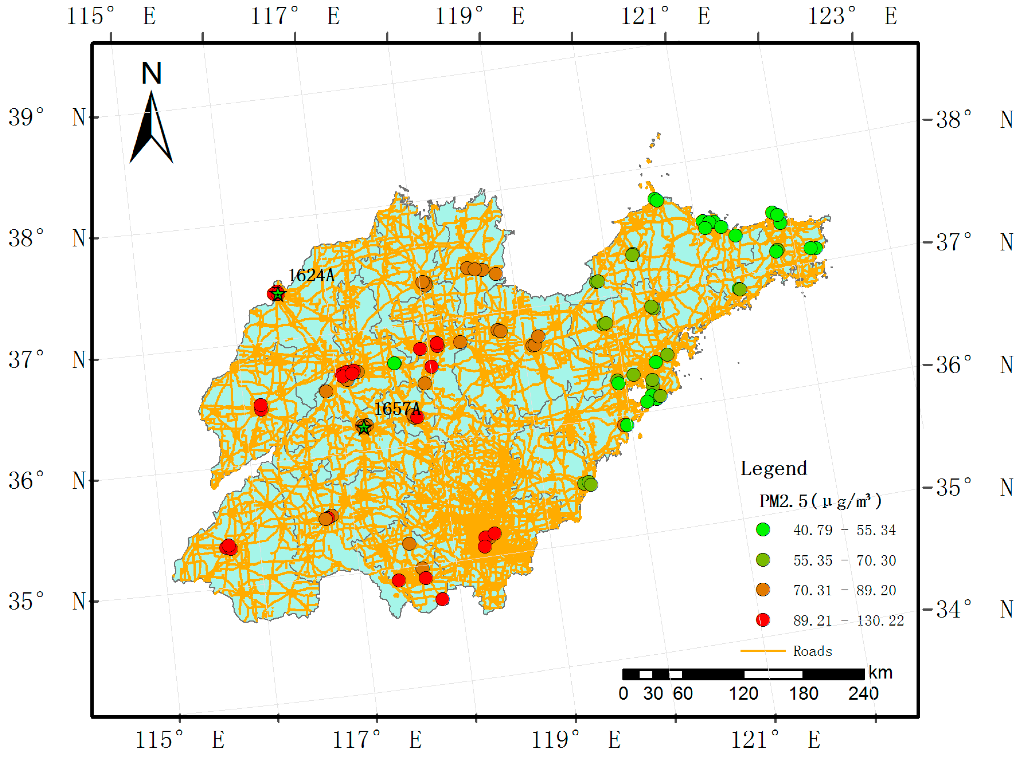
2.1. Study Domain
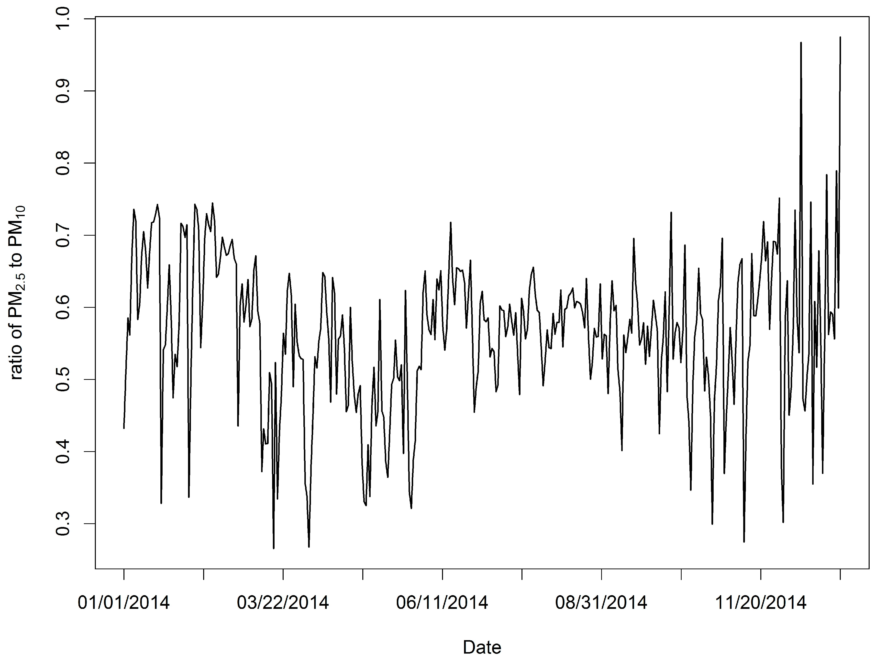
2.2. Monitoring Data
2.3. Predictors
2.4. Modeling Approach
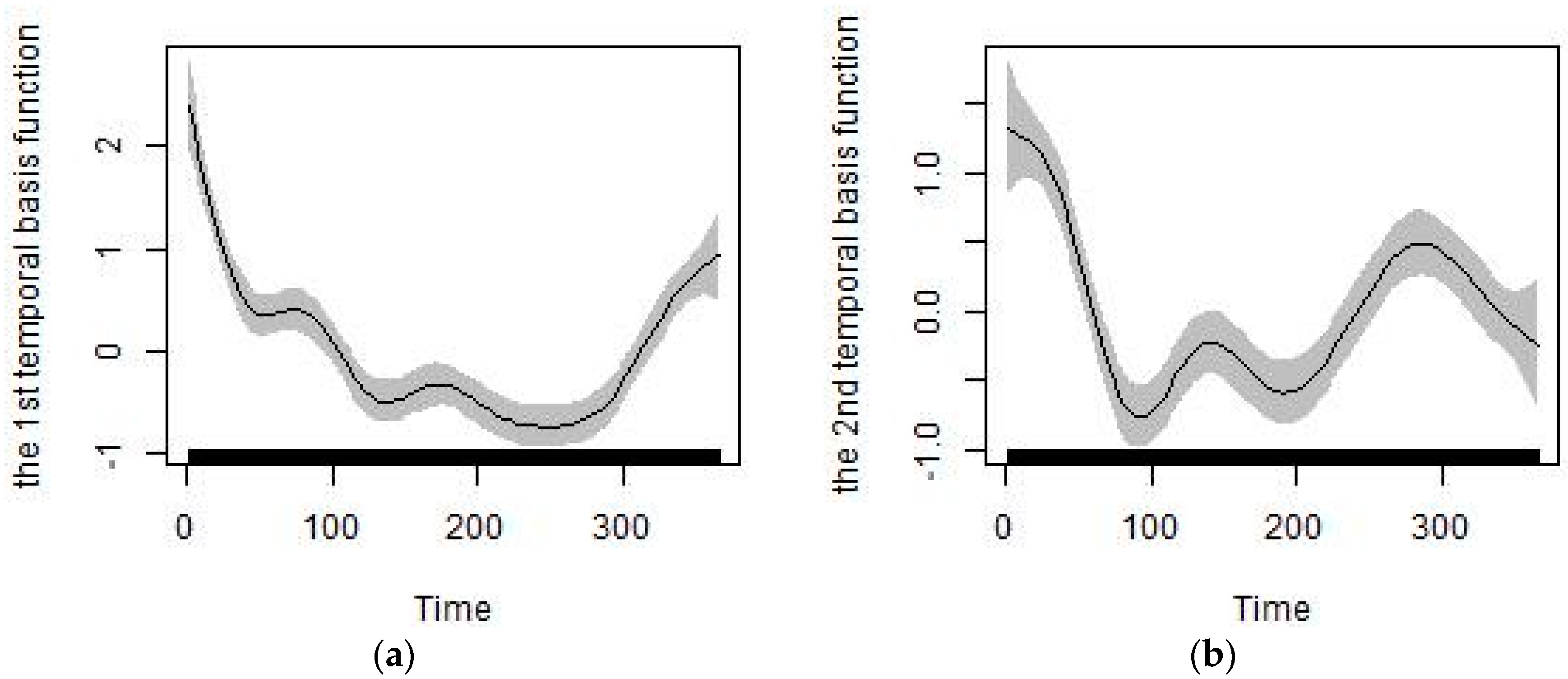
2.4.1. Generation of the Predictors of Temporal Trends
2.4.2. Non-Linear Additive Modeling
2.4.3. Ensemble Learning
2.4.4. Kriging of Spatiotemporal Residuals
2.4.5. Validation and Independent Test
3. Results
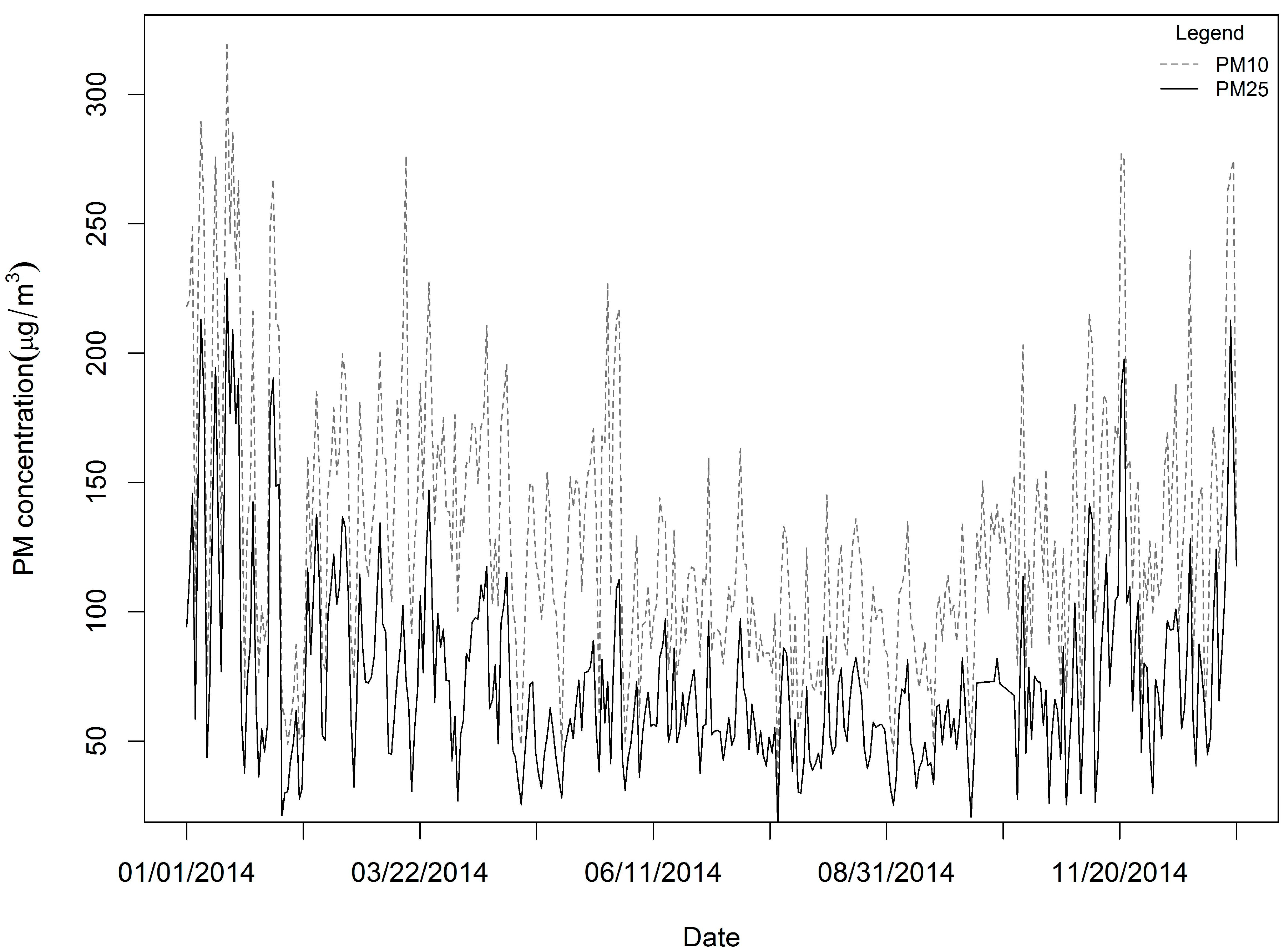
3.1. Data Summary
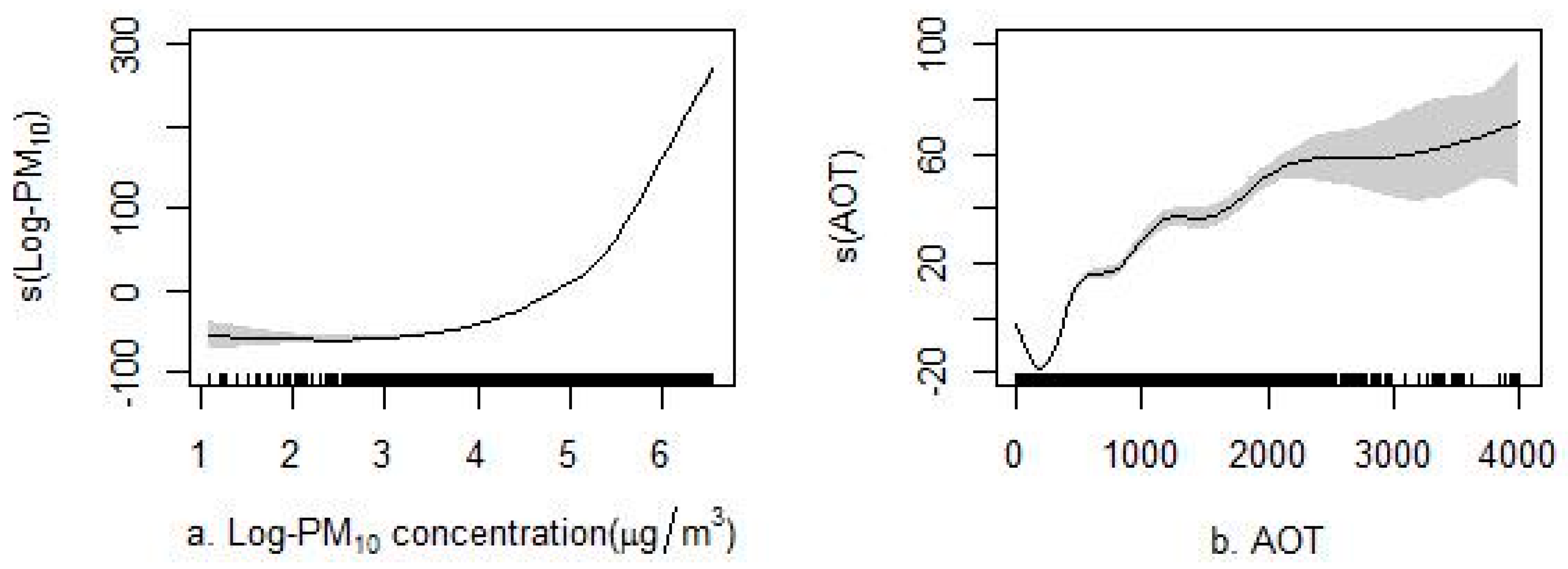
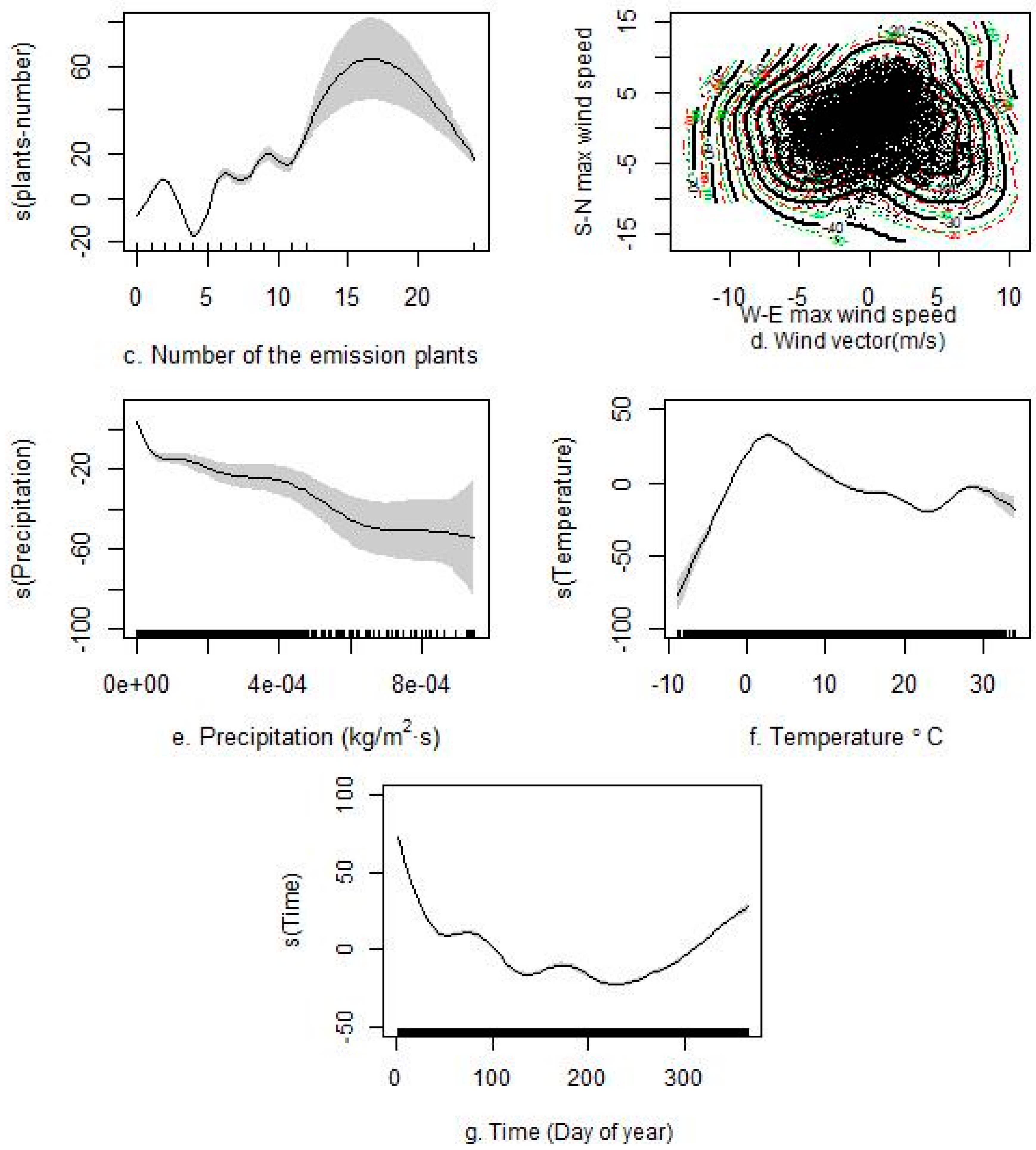
3.2. Predictors
3.3. Comparision of the Different Models and Independent Test
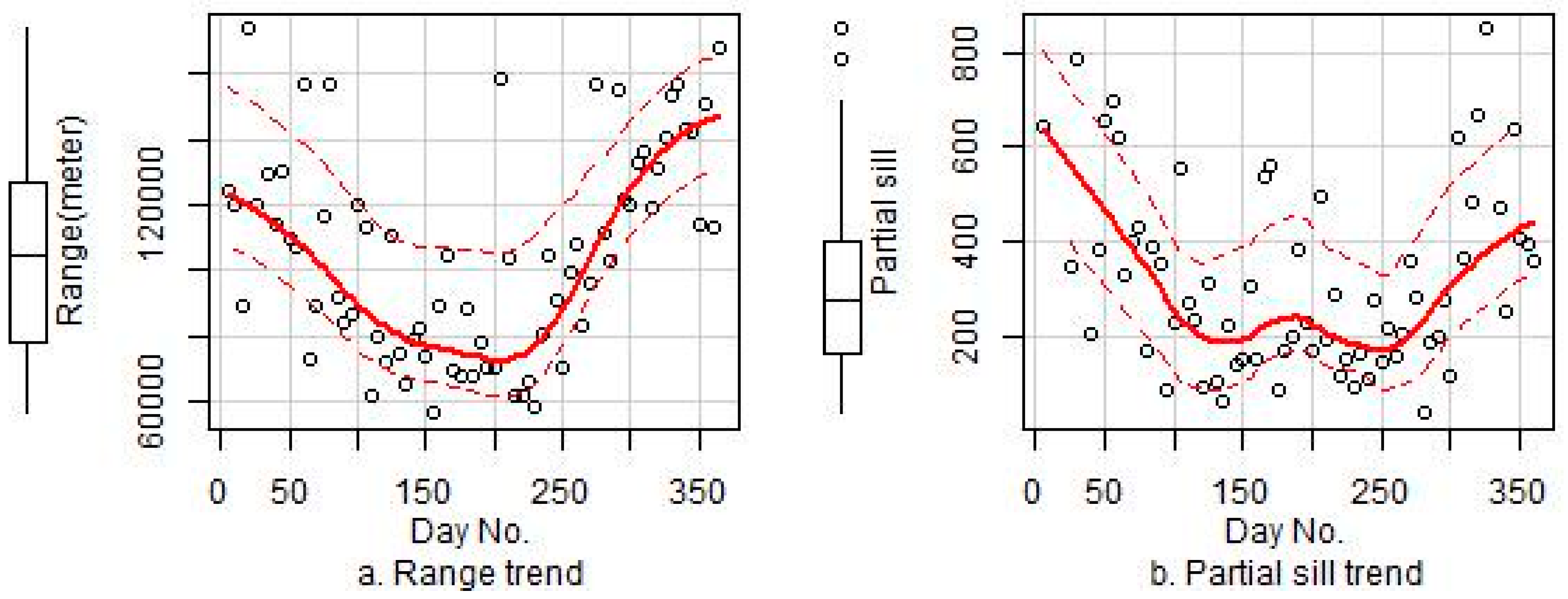
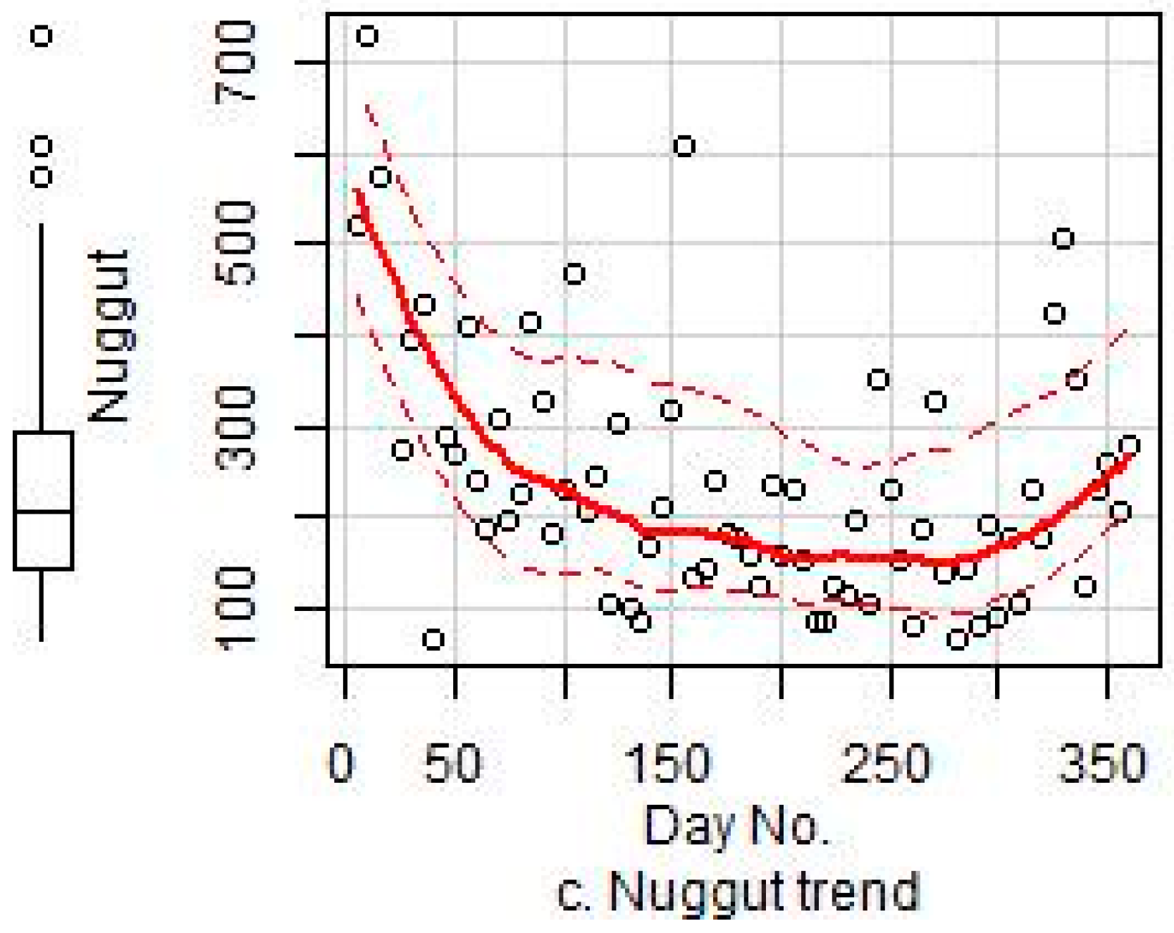
3.4. Variogram Modeling of the Residuals
3.5. Uncertainty
4. Discussion
5. Conclusions
Supplementary Materials
Acknowledgments
Author Contributions
Conflicts of Interest
References
- Bell, M.L. Assessment of the health impacts of particulate matter characteristics. Res. Rep. 2012, 161, 5–38. [Google Scholar]
- World Health Organization. Review of Evidence on Health Aspects of Air Pollution—REVIHAAP Project: Final Technical Report. Available online: http://www.euro.who.int/en/health-topics/environment-and-health/air-quality/publications/2013/review-of-evidence-on-health-aspects-of-air-pollution-revihaap-project-final-technical-report (accessed on 1 December 2016).
- World Health Organization. Health Effects of Particular Matter: Policy Implications for Countries in Eastern Europe, Caucasus and Central Asia; 2013. Available online: http://www.euro.who.int/en/health-topics/environment-and-health/air-quality/publications/2013/health-effects-of-particulate-matter.-policy-implications-for-countries-in-eastern-europe,-caucasus-and-central-asia-2013 (accessed on 1 December 2016).
- EPA. Criteria Air Pollutants; 2015. Available online: https://www.epa.gov/criteria-air-pollutants (accessed on 1 December 2016).
- Perrone, M.; Gualtieri, M.; Consonni, V.; Ferrero, L.; Sangiorgi, G.; Longhin, E.; Ballabio, D.; Bolzacchini, E.; Camatini, M. Particle size, chemical composition, seasons of the year and urban, rural or remote site origins as determinants of biological effects of particulate matter on pulmonary cells. Environ. Pollut. 2013, 176, 215–227. [Google Scholar] [CrossRef] [PubMed]
- Bono, R.; Tassinari, R.; Bellisario, V.; Gilli, G.; Pazzi, M.; Pirro, V.; Mengozzi, G.; Bugiani, M.; Piccioni, P. Urban air and tobacco smoke as conditions that increase the risk of oxidative stress and respiratory response in youth. Environ. Res. 2015, 137, 141–146. [Google Scholar] [CrossRef] [PubMed]
- Abbey, D.E.; Ostro, B.E.; Petersen, F.; Burchette, R.J. Chronic respiratory symptoms associated with estimated long-term ambient concentrations of fine particulates less than 2.5 microns in aerodynamic diameter (PM2.5) and other air pollutants. J. Expo. Anal. Environ. Epidemiol. 1994, 5, 137–159. [Google Scholar]
- Mar, T.F.; Jansen, K.; Shepherd, K.; Lumley, T.; Larson, T.V.; Koenig, J.Q. Exhaled nitric oxide in children with asthma and short-term PM2.5 exposure in Seattle. Environ. Health Perspect. 2005, 113, 1791–1794. [Google Scholar] [CrossRef] [PubMed]
- Nikasinovic, L.; Just, J.; Sahraoui, F.; Seta, N.; Grimfeld, A.; Momas, I. Nasal inflammation and personal exposure to fine particles PM2. 5 in asthmatic children. J. Allergy Clin. Immunol. 2006, 117, 1382–1388. [Google Scholar] [CrossRef] [PubMed]
- Tecer, L.H.; Alagha, O.; Karaca, F.; Tuncel, G.; Eldes, N. Particulate matter (PM2.5, PM10–2.5, and PM10) and children’s hospital admissions for asthma and respiratory diseases: A bidirectional case-crossover study. J. Toxicol. Environ. Health 2008, 71, 512–520. [Google Scholar] [CrossRef] [PubMed]
- Loomis, D.; Grosse, Y.; Lauby-Secretan, B.; El Ghissassi, F.; Bouvard, V.; Benbrahim-Tallaa, L.; Guha, N.; Baan, R.; Mattock, H.; Straif, K. The carcinogenicity of outdoor air pollution. Lancet Oncol. 2013, 14, 1262. [Google Scholar] [CrossRef]
- Brunekreef, B.; Janssen, N.; de Hartog, J.J.; Oldenwening, M.; Meliefste, K.; Hoek, G.; Lanki, T.; Timonen, K.L.; Vallius, M.; Pekkanen, J. Personal, indoor, and outdoor exposures to PM2.5 and its components for groups of cardiovascular patients in Amsterdam and Helsinki. Res. Rep. 2005, 127, 1–79. [Google Scholar]
- Dockery, D.W. Epidemiologic evidence of cardiovascular effects of particulate air pollution. Environ. Health Perspect. 2001, 109 (Suppl. 4), 483–486. [Google Scholar] [CrossRef] [PubMed]
- Liao, D.; Creason, J.; Shy, C.; Williams, R.; Watts, R.; Zweidinger, R. Daily variation of particulate air pollution and poor cardiac autonomic control in the elderly. Environ. Health Perspect. 1999, 107, 521–525. [Google Scholar] [CrossRef] [PubMed]
- Yuan, Y.; Liu, S.; Castro, R.; Xubin, P. PM2. 5 monitoring and mitigation in the cities of China. Environ. Sci. Technol. 2012, 46, 3627–3628. [Google Scholar] [CrossRef] [PubMed]
- Statistical Center of Beijing University. Assessment Report of Air Quality (In Chinese); Statistics Science Center of Beijing University: Beijing, China, 2015. [Google Scholar]
- Blanchard, C.L.; Tanenbaum, S.; Motallebi, N. Spatial and temporal characterization of PM2.5 mass concentrations in California, 1980–2007. J. Air Waste Manag. Assoc. 2011, 61, 339–351. [Google Scholar] [CrossRef] [PubMed]
- Lall, R.; Kendall, M.; Ito, K.; Thurston, D.G. Estimation of historical annual PM2.5 exposures for health effects assessment. Atmos. Environ. 2004, 38, 5217–5226. [Google Scholar] [CrossRef]
- Hoek, G.; Beelen, R.; de Hoogh, K.; Vienneau, D.; Gulliver, J.; Fischer, P. A review of land-use regression models to assess spatial variation of outdoor air pollution. Atmos. Environ. 2008, 42, 7561–7578. [Google Scholar] [CrossRef]
- Kim, S.Y.; Sheppard, L.; Kim, H. Health effects of long-term air pollution: Influence of exposure prediction methods. Epidemiology 2009, 20, 442–450. [Google Scholar] [CrossRef] [PubMed]
- Di, Q.; Kloog, I.; Koutrakis, P.; Lyapustin, A.; Wang, Y.J.; Schwartz, J. Assessing PM2.5 exposures with high spatiotemporal resolution across the continental United States. Environ. Sci. Technol. 2016, 50, 4712–4721. [Google Scholar] [CrossRef] [PubMed]
- Yuval; Broday, D.M. Enhancement of PM2.5 exposure estimation using PM10 observations. Environ. Sci. Proc. Imp. 2014, 16, 1094–1102. [Google Scholar] [CrossRef] [PubMed]
- Kloog, I.; Coull, B.A.; Zanobetti, A.; Koutrakis, P.; Schwartz, J.D. Acute and chronic effects of particles on hospital admissions in New England. PLoS ONE 2012, 7, e34664. [Google Scholar] [CrossRef] [PubMed]
- Xie, Y.; Wang, Y.; Zhang, K.; Dong, W.; Lv, B.; Bai, Y. Daily estimation of ground-level PM2.5 concentrations over Beijing using 3 km resolution MODIS AOD. Environ. Sci. Technol. 2015, 49, 12280–12288. [Google Scholar] [CrossRef] [PubMed]
- Zheng, Y.X.; Zhang, Q.; Liu, Y.; Geng, G.N.; He, K.B. Estimating ground-level PM2.5 concentrations over three megalopolises in China using satellite-derived aerosol optical depth measurements. Atmos. Environ. 2016, 124, 232–242. [Google Scholar] [CrossRef]
- Li, L.; Wu, J.; Hudda, N.; Sioutas, C.; Fruin, S.A.; Delfino, R.J. Modeling the concentrations of on-road air pollutants in Southern California. Environ. Sci. Technol. 2013, 47, 9291–9299. [Google Scholar] [CrossRef] [PubMed]
- Troyanskaya, O.; Cantor, M.; Sherlock, G.; Brown, P.; Hastie, T.; Tibshirani, R.; Botstein, D.; Altman, R.B. Missing value estimation methods for DNA microarrays. Bioinformatics 2001, 17, 520–525. [Google Scholar] [CrossRef] [PubMed]
- Bayraktar, H.; Turalioğlu, F.S.; Tuncel, G. Average mass concentrations of TSP, PM10 and PM2.5 in Erzurum urban atmosphere, Turkey. Stoch. Environ. Res. Risk Assess. 2008, 24, 57–65. [Google Scholar] [CrossRef]
- Tai, A.P.K.; Mickley, L.J.; Jacob, D.J. Correlations between fine particulate matter (PM2.5) and meteorological variables in the United States: Implications for the sensitivity of PM2.5 to climate change. Atmos. Environ. 2010, 44, 3976–3984. [Google Scholar] [CrossRef]
- Tai, A.P.K.; Mickley, L.J.; Jacob, D.J.; Leibensperger, E.M.; Zhang, L.; Fisher, J.A.; Pye, H.O.T. Meteorological modes of variability for fine particulate matter (PM2.5) air quality in the United States: Implications for PM2.5 sensitivity to climate change. Atmos. Chem. Phys. 2011, 13, 3131–3145. [Google Scholar] [CrossRef]
- Liu, Y.; Paciorek, C.J.; Koutrakis, P. Estimating regional spatial and temporal variability of PM2.5 concentrations using satellite data, meteorology, and land use information. Environ. Health Perspect. 2009, 117, 886. [Google Scholar] [CrossRef] [PubMed]
- Dawson, J.P.; Adams, P.J.; Pandis, S.N. Sensitivity of PM2.5 to climate in the eastern us: A modeling case study. Atmos. Chem. Phys. 2007, 7, 4295–4309. [Google Scholar] [CrossRef]
- Bosilovich, M.G.; Lucchesi, R.; Suarez, M. Merra-2: File Specification. 2015. Available online: https://ntrs.nasa.gov/search.jsp?R=20150019760 (accessed on 1 December 2016).
- Global Modeling and Assimilation Office (GMAO). M2T1NXFLX. Available online: https://disc.sci.gsfc.nasa.gov/uui/datasets?keywords=M2T1NXFLX_V5.12.4 (accessed on 1 July 2016).
- Wang, X.; Bi, X.; Sheng, G.; Fu, J. Chemical composition and sources of PM10 and PM2.5 aerosols in Guangzhou, China. Environ. Monit. Assess. 2006, 119, 425–439. [Google Scholar] [CrossRef] [PubMed]
- Giugliano, M.; Lonati, G.; Butelli, P.; Romele, L.; Tardivo, R.; Grosso, M. Fine particulate (PM2.5–PM1) at urban sites with different traffic exposure. Atmos. Environ. 2005, 39, 2421–2431. [Google Scholar] [CrossRef]
- Querol, X.; Alastuey, A.; Ruiz, C.R.; Artiñano, B.; Hansson, H.C.; Harrison, R.M.; Buringh, E.; Brink, H.M.T.; Lutz, M.; Bruckmann, P. Speciation and origin of PM10 and PM2.5 in selected European cities. J. Aerosol Sci. 2004, 38, 6547–6555. [Google Scholar] [CrossRef]
- Fusheng, W.; Enjiang, T.; Guoping, W.; Wei, H.; Wilson, W.E.; Chapman, R.S.; Pau, J.C.; Zhang, J. Concentrations and elemental components of PM2.5 and PM10 in ambient air in four large Chinese cities. Environ. Monit. China 2001, 17, 1–6. (In Chinese) [Google Scholar]
- Chinese Academy of Sciences (RESDC). Available online: http://www.resdc.cn (accessed on 1 July 2016).
- NASA Center for Climate Simulation. Available online: ftp://dataportal.nccs.nasa.gov/DataRelease/ (accessed on 1 July 2016).
- Ma, Z.; Hu, X.; Sayer, A.M.; Levy, R.; Zhang, Q.; Xue, Y.; Tong, S.; Bi, J.; Huang, L.; Liu, Y. Satellite-based spatiotemporal trends in PM2.5 concentrations: China, 2004–2013. Environ. Health Perspect. 2016, 124, 184–193. [Google Scholar] [CrossRef] [PubMed]
- Wang, J. Intercomparison between satellite-derived aerosol optical thickness and PM2.5 mass: Implications for air quality studies. Geophys. Res. Lett. 2003, 30, 267–283. [Google Scholar] [CrossRef]
- Geospatal Data Cloud. Available online: http://www.gscloud.cn (accessed on 1 July 2016).
- Jiang, M.; Weiwei, S. Investigating Metrological and Geographical Effect in Remote Sensing Retrival of PM2.5 Concentration in Yangtze River Delta. In Proceedings of the Geoscience and Remote Sensing Symposium (IGARSS), Beijing, China, 10–15 July 2016; pp. 4108–4111. [Google Scholar]
- O’brien, R.M. A caution regarding rules of thumb for variance inflation factors. Qual. Quant. 2007, 41, 673–690. [Google Scholar] [CrossRef]
- Bozdogan, H. Model selection and Akanke’s information criterion (AIC): The general theory and its analytical extensions. Psychometrika 1987, 52, 345–370. [Google Scholar] [CrossRef]
- Yang, Y.; Christakos, G. Spatiotemporal characterization of ambient PM2.5 concentrations in Shandong province (China). Environ. Sci. Technol. 2015, 49, 13431–13438. [Google Scholar] [CrossRef] [PubMed]
- Huang, N.E.; Shen, Z.; Long, S.R.; Wu, M.C.; Shih, H.H.; Zheng, Q.; Yen, N.-C.; Tung, C.C.; Liu, H.H. The empirical mode decomposition and the Hilbert spectrum for nonlinear and non-stationary time series analysis. Proc. Math. Phys. Eng. Sci. 1998, 903–995. [Google Scholar] [CrossRef]
- Li, L.; Wu, J.; Ghosh, J.K.; Ritz, B. Estimating Spatiotemporal Variability of Ambient Air Pollutant Concentrations with a Hierarchical Model. Atmos. Environ. 2013, 71, 54–63. [Google Scholar] [CrossRef] [PubMed]
- Onorati, R.; Sampson, P.; Guttorp, P. A spatio-temporal model based on the SVD to analyze daily average temperature across the Sicily region. J. Environ. Stat. 2013, 5. [Google Scholar]
- Lindstrom, J.; Szpiro, A.A.; Sampson, P.D.; Sheppard, L.; Oron, A.; Richards, M.; Larson, T. A Flexible Spatio-Temporal Model for Air Pollution: Allowing for Spatio-Temporal Covariates. UW Biostatistics Working Paper Series. 2011. Available online: http://lup.lub.lu.se/record/4730139 (accessed on 1 December 2016).
- Dietterich, T.G. Ensemble methods in machine learning. Mult. Classifier Syst. 2000, 1857, 1–15. [Google Scholar] [CrossRef]
- Bühlmann, P.; Hothorn, T. Boosting algorithms: Regularization, prediction and model fitting. Stat. Sci. 2007, 22, 477–505. [Google Scholar] [CrossRef]
- Liaw, A.; Wiener, M. Classification and regression by randomforest. R News 2002, 2, 18–22. [Google Scholar]
- Peters, A.; Hothorn, T.; Lausen, B. Ipred: Improved predictors. R News 2002, 2, 33–36. [Google Scholar]
- Ridgeway, G. The state of boosting. Comput. Sci. Stat. 1999, 172–181. [Google Scholar]
- Breiman, L. Bagging predictors. Mach. Learn. 1996, 24, 123–140. [Google Scholar] [CrossRef]
- Aslam, J.; Popa, R.; Rivest, R. On estimating the size and confidence of a statistical audit. EVT 2007, 7, 8. [Google Scholar]
- Christakos, G. A Bayesian maximum entropy view to the spatial estimation problem. Math. Geol. 1990, 22, 763–777. [Google Scholar] [CrossRef]
- Goovaerts, P. Geostatistics for Natural Resources Evaluation; Oxford University Press: New York, NY, USA, 1997; ISBN 9780195115383. [Google Scholar]
- Chiles, P.J.; Delfiner, P. Geostatistics: Modeling Spatial Uncertainty; John Wiley & Sons: New York, NY, USA, 1999; ISBN 0-471-08315-1. [Google Scholar]
- Johnston, K.; Hoef, M.J.; Krivoruchko, K.; Lucas, N. ArcGIS 9: Using ArcGIS Geostatistical Analyst; ESRI Press: Sacramento, CA, USA, 2004; ISBN 9781589481060. [Google Scholar]
- Bell, S. A beginner’s Guide to Uncertainty of Measurement; National Physical Laboratory: Teddington, UK, 2001; ISBN 1368-6550. [Google Scholar]
- Kalla, S. Measurement of Uncertainty: Standard Deviation. Available online: https://explorable.com/measurement-of-uncertainty-standard-deviation (accessed on 11 December 2016).
- Kloog, I.; Koutrakis, P.; Coull, B.A.; Lee, H.J.; Schwartz, J. Assessing temporally and spatially resolved PM2.5 exposures for epidemiological studies using satellite aerosol optical depth measurements. Atmos. Environ. 2011, 45, 6267–6275. [Google Scholar] [CrossRef]
- Zang, Z.; Wang, W.; You, W.; Li, Y.; Ye, F.; Wang, C. Estimating ground-level PM2.5 concentrations in Beijing, China using aerosol optical depth and parameters of the temperature inversion layer. Sci. Total Environ. 2017, 575, 1219–1227. [Google Scholar] [CrossRef] [PubMed]
- Raffuse, S.; McCarthy, M.; Craig, K.; DeWinter, J.; Jumbam, L.; Fruin, S.; Gauderman, J.; Lurmann, F. High-resolution MODIS aerosol retrieval during wildfire events in California for use in exposure assessment. J. Geophys. Res. Atmos. 2013, 118, 11242–11255. [Google Scholar] [CrossRef]
- Watson, J.G.; Chow, J.C.; Shah, J.J. Analysis of Inhalable and Fine Particulate Matter Measurements; National Tech Information Service: Alexandria, VA, USA, 1981; ISBN 9781249430346. [Google Scholar]
- Jerrett, M.; Burnett, R.; Pope, A.; Krewski, D.; Thurston, G.; Christakos, G.; Hughes, E.; Ross, Z.; Shi, Y.; Thun, M. Spatiotemporal Analysis of Air Pollution and Mortality in California Based on the American Cancer Society Cohort: Final Report; State of California Air Resources Board: Sacramento, CA, USA, 2012. [Google Scholar]
- Robichaud, A.; Ménard, R. Multi-year objective analyses of warm season ground-level ozone and PM2.5 over North America using real-time observations and Canadian operational air quality models. Atmos. Chem. Phys. 2014, 14, 1769–1800. [Google Scholar] [CrossRef]
- Li, L.; Wu, A.; Cheng, I.; Wu, J. Spatiotemporal Estimation of Historical 1 PM2.5 Concentrations Using PM10, Meteorological Variables, and Spatial Effect. Atmos. Environ. 2017. under review. [Google Scholar]


| Predictive Variable (Unit) | Variance Explained in the Univariate Model | Variance Explained in the Multivariate Model (without PM10) | Variance Explained in the Multivariate Model (Including PM10) |
|---|---|---|---|
| PM10 (g/m3) | 73.00% | - | 67.97% |
| Aerosol optical thickness (AOT) | 7.38% | 4.77% | 0.48% |
| Normalized difference vegetation index (NDVI) | 3.14% | 0.24% | 0.24% |
| Precipitation (kg/m2s) | 1.75% | 0.02% | 0.02% |
| Temperature (°C) | 1.08% | 2.62% | 0.48% |
| Mean specific humidity (kg/kg) | 9.08% | 0.48% | 0.48% |
| Roadway length within the 10 km buffer of a monitoring station (m) | 2.62% | 2.86% | 1.45% |
| Shortest distance of roadway to a monitoring station (m) | 1.73% | 2.15% | 1.21% |
| Wind speed vector | 3.76% | 1.43% | 0.48% |
| Area proportion of the factories and mines, oil fields and stone-pit land-use | 2.29% | 2.15% | 0.73% |
| Area proportion of the forest land-use | 2.06% | 2.62% | 0.48% |
| Number of the emission plants | 4.48% | 1.67% | 0.97% |
| Shortest distance to the emission plants | 1.70% | 1.67% | 0.24% |
| The first temporal basis function | 37.00% | 26.71% | 4.84% |
| The second temporal basis function | 5.79% | 1.43% | 0.48% |
| Time (day of year) | 14.70% | 2.38% | 0.73% |
| Total | 53.20% | 81.30% |
| Model | Use of Predictive Variables and Residual Kriging | R2 | CV a R2 | CV RMSE b (g/m3) |
|---|---|---|---|---|
| Model 1 | GAM with no use of PM10 data and residual kriging | 0.53 | 0.53 | 34.69 |
| Model 2 | GAM with PM10 data but without residual kriging | 0.81 | 0.81 | 21.87 |
| Model 3 | Bagging without PM10 data and residual kriging | 0.53 | 34.79 | |
| Model 4 | Bagging without PM10 data but with residual kriging | 0.86 | 18.85 | |
| Model 5 | Bagging with PM10 data but without residual kriging | 0.82 | 21.82 | |
| Model 6 | Bagging with PM10 data and residual kriging | 0.89 | 17.06 |
| Model | Parameter | Minimum | 1st Qu. a | Median | Mean | 3rd Qu. a | Maximum |
|---|---|---|---|---|---|---|---|
| Model 4 | Range | 5551 | 63,780 | 93,050 | 107,100 | 137,000 | 712,900 |
| Partial sill | 1.65 | 96.18 | 208 | 448.7 | 507 | 6560 | |
| Nugget | 20.74 | 97.12 | 159.6 | 260.4 | 284.3 | 3096 | |
| Model 6 | Range | 4250 | 60,350 | 95,660 | 103,100 | 144,500 | 475,200 |
| Partial sill | 0.0839 | 29.7 | 71.27 | 144.4 | 162.3 | 2866 | |
| Nugget | 0.0912 | 85.33 | 146.6 | 228.1 | 264.5 | 2650 |
| Model | Minimum | 1st Qu. a | Median | Mean | 3rd Qu. a | Max. |
|---|---|---|---|---|---|---|
| Models 3 and 4 | 0.43 | 1.33 | 1.80 | 2.18 | 2.54 | 21.43 |
| Models 5 and 6 | 0.26 | 0.79 | 1.19 | 1.47 | 1.76 | 26.81 |
© 2017 by the authors. Licensee MDPI, Basel, Switzerland. This article is an open access article distributed under the terms and conditions of the Creative Commons Attribution (CC BY) license (http://creativecommons.org/licenses/by/4.0/).
Share and Cite
Li, L.; Zhang, J.; Qiu, W.; Wang, J.; Fang, Y. An Ensemble Spatiotemporal Model for Predicting PM2.5 Concentrations. Int. J. Environ. Res. Public Health 2017, 14, 549. https://doi.org/10.3390/ijerph14050549
Li L, Zhang J, Qiu W, Wang J, Fang Y. An Ensemble Spatiotemporal Model for Predicting PM2.5 Concentrations. International Journal of Environmental Research and Public Health. 2017; 14(5):549. https://doi.org/10.3390/ijerph14050549
Chicago/Turabian StyleLi, Lianfa, Jiehao Zhang, Wenyang Qiu, Jinfeng Wang, and Ying Fang. 2017. "An Ensemble Spatiotemporal Model for Predicting PM2.5 Concentrations" International Journal of Environmental Research and Public Health 14, no. 5: 549. https://doi.org/10.3390/ijerph14050549
APA StyleLi, L., Zhang, J., Qiu, W., Wang, J., & Fang, Y. (2017). An Ensemble Spatiotemporal Model for Predicting PM2.5 Concentrations. International Journal of Environmental Research and Public Health, 14(5), 549. https://doi.org/10.3390/ijerph14050549