The Potential Impact of Satellite-Retrieved Cloud Parameters on Ground-Level PM2.5 Mass and Composition


Abstract
:1. Introduction
2. Materials and Methods
3. Results
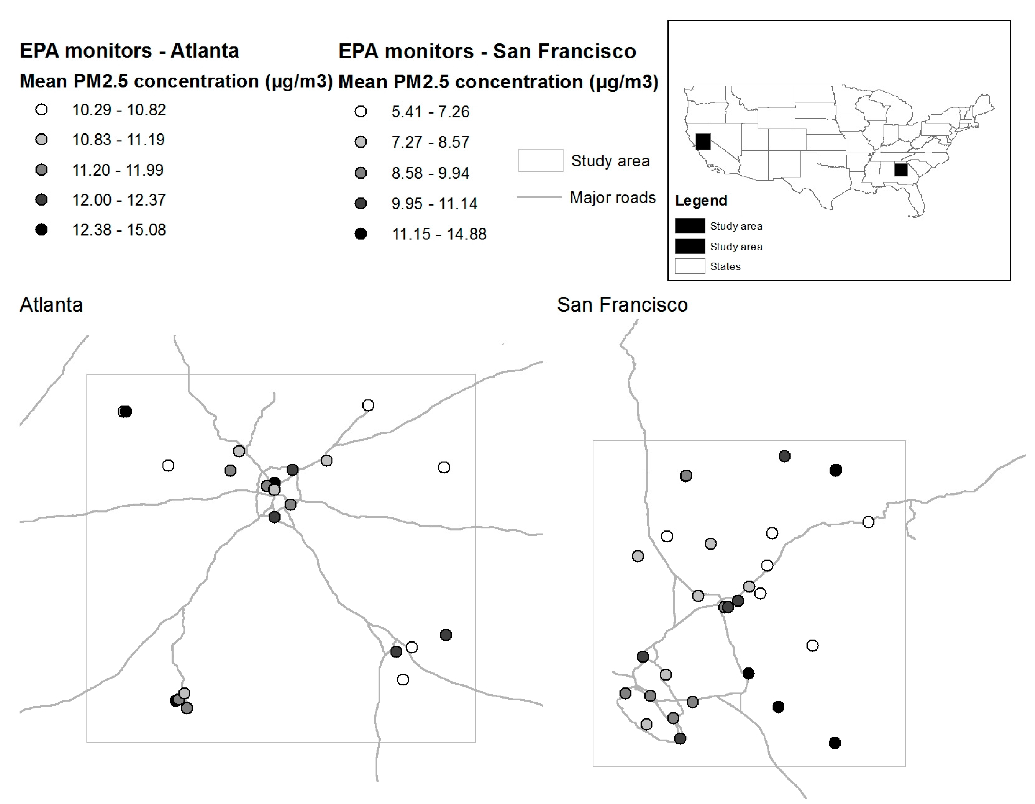
3.1. Study Area Characteristics
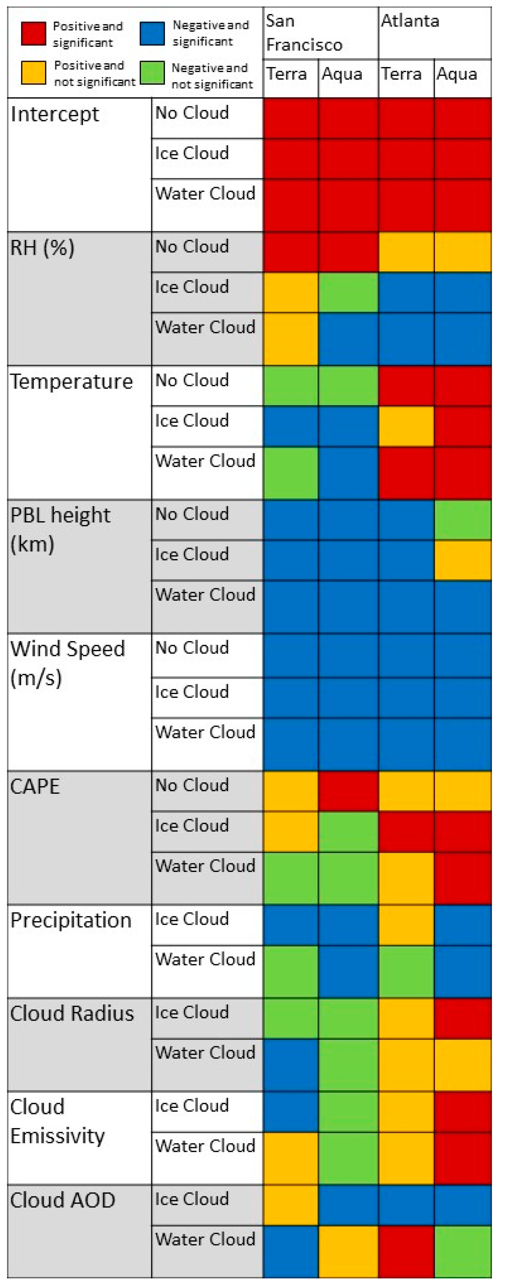
3.2. Clouds and 24-Hour Gravimetric Mass
3.3. Clouds and Speciation of PM2.5
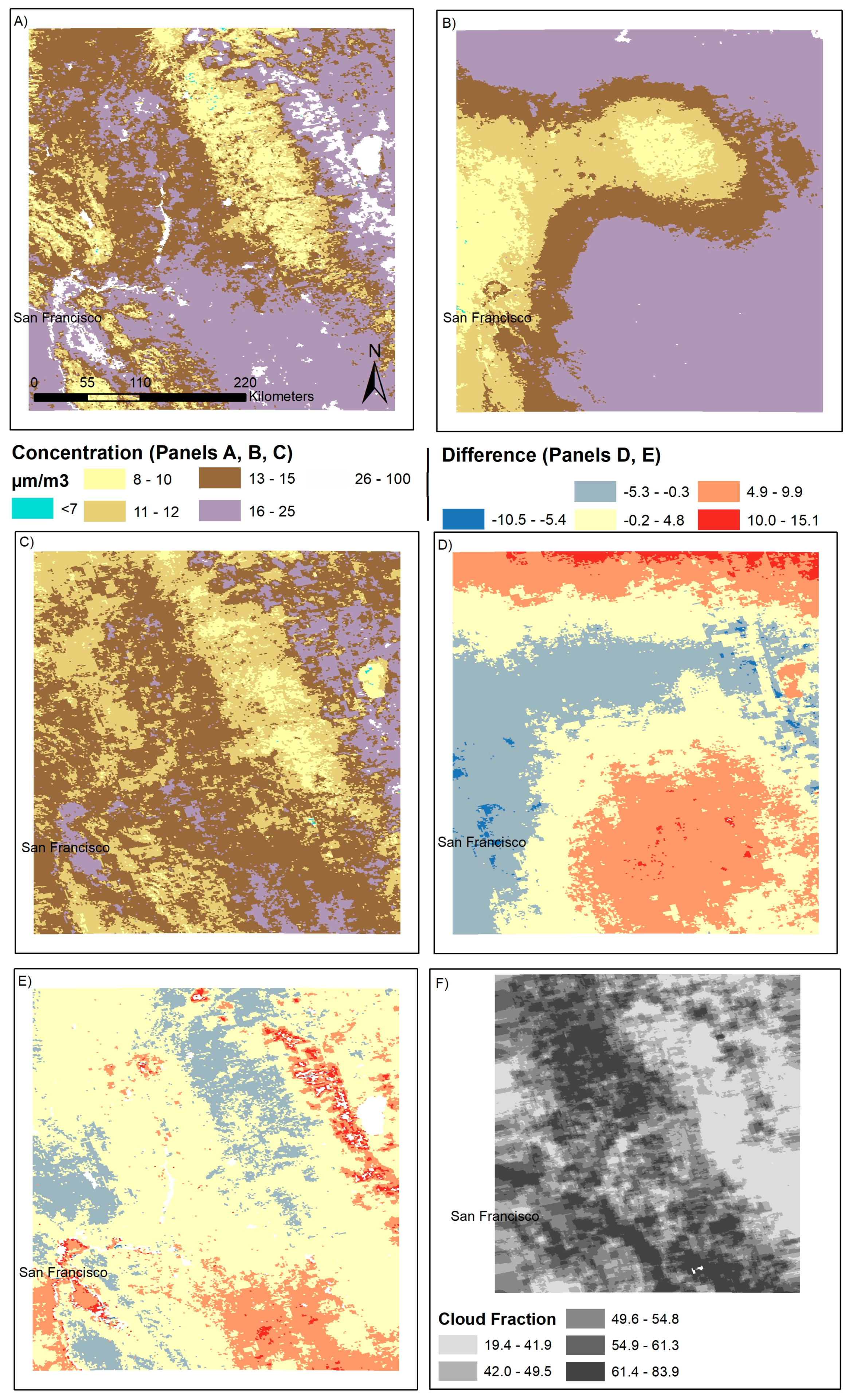
3.4. Application to MAIAC-Derived PM2.5
4. Discussion
5. Conclusions
Supplementary Materials
Acknowledgments
Author Contributions
Conflicts of Interest
References
- Sorek-Hamer, M.; Just, A.C.; Kloog, I. Satellite remote sensing in epidemiological studies. Curr. Opin. Pediatr. 2016, 28, 228–234. [Google Scholar] [CrossRef] [PubMed]
- Fasso, A.; Finazzi, F. Statistical Mapping of Air Quality by Remote Sensing. In Proceedings of the Accuracy 2010 Conference, leicester, UK, 20–23 July 2010; Available online: http://www.spatial-accuracy.org/FassoAccuracy2010 (accessed on 17 October 2017).
- Belle, J.; Liu, Y. Evaluation of aqua modis collection 6 aod parameters for air quality research over the continental united states. Remote Sens. 2016, 8, 815. [Google Scholar] [CrossRef]
- Anderson, T.L.; Charlson, R.J.; Winker, D.M.; Ogren, J.A.; Holmén, K. Mesoscale variations of tropospheric aerosols. J. Atmos. Sci. 2003, 60, 119–136. [Google Scholar] [CrossRef]
- Just, A.C.; Wright, R.O.; Schwartz, J.; Coull, B.A.; Baccarelli, A.A.; Tellez-Rojo, M.M.; Moody, E.; Wang, Y.; Lyapustin, A.; Kloog, I. Using high-resolution satellite aerosol optical depth to estimate daily PM2.5 geographical distribution in mexico city. Environ. Sci. Technol. 2015, 49, 8576–8584. [Google Scholar] [CrossRef] [PubMed]
- Ford, B.; Heald, C. Exploring the uncertainty associated with satellite-based estimates of premature mortality due to exposure to fine particulate matter. Atmos. Chem. Phys. Discuss. 2015, 15, 25329–25380. [Google Scholar] [CrossRef]
- Van Donkelaar, A.; Martin, R.V.; Brauer, M.; Boys, B.L. Use of satellite observations for long-term exposure assessment of global concentrations of fine particulate matter. Environ. Health Perspect. 2015, 123, 135. [Google Scholar] [CrossRef] [PubMed]
- Christopher, S.A.; Gupta, P. Satellite remote sensing of particulate matter air quality: The cloud-cover problem. J. Air Waste Manag. Assoc. 2010, 60, 596–602. [Google Scholar] [CrossRef] [PubMed]
- Gupta, P.; Christopher, S.A. An evaluation of terra-modis sampling for monthly and annual particulate matter air quality assessment over the southeastern united states. Atmos. Environ. 2008, 42, 6465–6471. [Google Scholar] [CrossRef]
- Yu, C.; Di Girolamo, L.; Chen, L.; Zhang, X.; Liu, Y. Statistical evaluation of the feasibility of satellite-retrieved cloud parameters as indicators of PM2.5 levels. J. Expo. Sci. Environ. Epidemiol. 2015, 25, 457–466. [Google Scholar] [CrossRef] [PubMed]
- Strickland, M.; Hao, H.; Hu, X.; Chang, H.; Darrow, L.; Liu, Y. Pediatric emergency visits and short-term changes in PM2.5 concentrations in the us state of georgia. Environ. Health Perspect. 2015, 124, 690–696. [Google Scholar] [CrossRef] [PubMed]
- Seinfeld, J.H.; Pandis, S.N. Atmospheric Chemistry and Physics: From Air Pollution to Climate Change; John Wiley & Sons: New York, NY, USA, 2012. [Google Scholar]
- Mauger, G.S.; Norris, J.R. Meteorological bias in satellite estimates of aerosol-cloud relationships. Geophys. Res. Lett. 2007, 34. [Google Scholar] [CrossRef]
- Rossow, W.B.; Schiffer, R.A. Advances in understanding clouds from ISCCP. Bull. Am. Meteorol. Soc. 1999, 80, 2261–2287. [Google Scholar] [CrossRef]
- Klein, S.A.; Hartmann, D.L.; Norris, J.R. On the relationships among low-cloud structure, sea surface temperature, and atmospheric circulation in the summertime northeast pacific. J. Clim. 1995, 8, 1140–1155. [Google Scholar] [CrossRef]
- Zhang, H.; Surratt, J.; Lin, Y.; Bapat, J.; Kamens, R. Effect of relative humidity on soa formation from isoprene/no photooxidation: Enhancement of 2-methylglyceric acid and its corresponding oligoesters under dry conditions. Atmos. Chem. Phys. 2011, 11, 6411–6424. [Google Scholar] [CrossRef]
- Zhou, Y.; Zhang, H.; Parikh, H.M.; Chen, E.H.; Rattanavaraha, W.; Rosen, E.P.; Wang, W.; Kamens, R.M. Secondary organic aerosol formation from xylenes and mixtures of toluene and xylenes in an atmospheric urban hydrocarbon mixture: Water and particle seed effects (II). Atmos. Environ. 2011, 45, 3882–3890. [Google Scholar] [CrossRef]
- Morgan, W.; Allan, J.; Bower, K.; Capes, G.; Crosier, J.; Williams, P.; Coe, H. Vertical distribution of sub-micron aerosol chemical composition from north-western europe and the north-east atlantic. Atmos. Chem. Phys. 2009, 9, 5389–5401. [Google Scholar] [CrossRef]
- Hicks, B.; Baldocchi, D.; Meyers, T.; Hosker, R.; Matt, D. A preliminary multiple resistance routine for deriving dry deposition velocities from measured quantities. Water Air Soil Pollut. 1987, 36, 311–330. [Google Scholar] [CrossRef]
- Ng, N.; Kwan, A.; Surratt, J.; Chan, A.; Chhabra, P.; Sorooshian, A.; Pye, H.O.; Crounse, J.; Wennberg, P.; Flagan, R. Secondary organic aerosol (SOA) formation from reaction of isoprene with nitrate radicals (NO3). Atmos. Chem. Phys. 2008, 8, 4117–4140. [Google Scholar] [CrossRef]
- Liao, H.; Adams, P.J.; Chung, S.H.; Seinfeld, J.H.; Mickley, L.J.; Jacob, D.J. Interactions between tropospheric chemistry and aerosols in a unified general circulation model. J. Geophys. Res. Atmos. 2003, 108. [Google Scholar] [CrossRef]
- Radke, L.F.; Hobbs, P.V.; Eltgroth, M.W. Scavenging of aerosol particles by precipitation. J. Appl. Meteorol. 1980, 19, 715–722. [Google Scholar] [CrossRef]
- Rodhe, H.; Grandell, J. On the removal time of aerosol particles from the atmosphere by precipitation scavenging. Tellus 1972, 24, 442–454. [Google Scholar] [CrossRef]
- Fan, J.; Leung, L.R.; Rosenfeld, D.; Chen, Q.; Li, Z.; Zhang, J.; Yan, H. Microphysical effects determine macrophysical response for aerosol impacts on deep convective clouds. Proc. Natl. Acad. Sci. USA 2013, 110, E4581–E4590. [Google Scholar] [CrossRef] [PubMed]
- Stevens, B.; Feingold, G. Untangling aerosol effects on clouds and precipitation in a buffered system. Nature 2009, 461, 607–613. [Google Scholar] [CrossRef] [PubMed]
- EPA. Aqs Data Mart. Available online: https://aqs.epa.gov/aqsweb/documents/data_mart_welcome.html (accessed on 31 March 2016).
- Hand, J.; Copeland, S.; Day, D.; Dillner, A.; Indresand, H.; Malm, W.; McDade, C.; Moore, C.; Pitchford, M.; Schichtel, B. Spatial and Seasonal Patterns and Temporal Variability of Haze and Its Constituents in the United States Report V. IMPROVE Reports. Available online: http://vista.cira.colostate.edu/improve/Publications/improve_reports.htm (accessed 11 September 2011).
- Malm, W.C.; Schichtel, B.A.; Pitchford, M.L. Uncertainties in PM2.5 gravimetric and speciation measurements and what we can learn from them. J. Air Waste Manag. Assoc. 2011, 61, 1131–1149. [Google Scholar] [CrossRef] [PubMed]
- Levy, R.; Mattoo, S.; Munchak, L.; Remer, L.; Sayer, A.; Hsu, N. The collection 6 modis aerosol products over land and ocean. Atmos. Meas. Tech. 2013, 6, 2989–3034. [Google Scholar] [CrossRef]
- Lyapustin, A.; Wang, Y.; Laszlo, I.; Kahn, R.; Korkin, S.; Remer, L.; Levy, R.; Reid, J. Multiangle implementation of atmospheric correction (MAIAC): 2. Aerosol algorithm. J. Geophys. Res. Atmos. 2011, 116. [Google Scholar] [CrossRef]
- Platnick, S.; Ackerman, S.; King, M.; Menzel, P.; Wind, G.; Frey, R. MODIS Atmosphere l2 Cloud Product (06_L2); System, N.M.A.P., Ed.; Goddard Space Flight Center: Greenbelt, MD, USA, 2015.
- Benjamin, S.G.; Dévényi, D.; Weygandt, S.S.; Brundage, K.J.; Brown, J.M.; Grell, G.A.; Kim, D.; Schwartz, B.E.; Smirnova, T.G.; Smith, T.L. An hourly assimilation-forecast cycle: The ruc. Mon. Weather Rev. 2004, 132, 495–518. [Google Scholar] [CrossRef]
- Benjamin, S.G.; Weygandt, S.S.; Brown, J.M.; Hu, M.; Alexander, C.R.; Smirnova, T.G.; Olson, J.B.; James, E.P.; Dowell, D.C.; Grell, G.A. A north american hourly assimilation and model forecast cycle: The rapid refresh. Mon. Weather Rev. 2016, 144, 1669–1694. [Google Scholar] [CrossRef]
- Grün, B.; Leisch, F. Fitting finite mixtures of generalized linear regressions in R. Comput. Stat. Data Anal. 2007, 51, 5247–5252. [Google Scholar] [CrossRef]
- Leisch, F. Flexmix: A General Framework for Finite Mixture Models and Latent Glass Regression in R. J. Stat. Softw. 2004, 11, 1–18. [Google Scholar] [CrossRef]
- Hu, X.; Waller, L.A.; Lyapustin, A.; Wang, Y.; Al-Hamdan, M.Z.; Crosson, W.L.; Estes, M.G.; Estes, S.M.; Quattrochi, D.A.; Puttaswamy, S.J. Estimating ground-level PM2.5 concentrations in the southeastern united states using maiac aod retrievals and a two-stage model. Remote Sens. Environ. 2014, 140, 220–232. [Google Scholar] [CrossRef]
- Kloog, I.; Ridgway, B.; Koutrakis, P.; Coull, B.A.; Schwartz, J.D. Long-and short-term exposure to PM2.5 and mortality: Using novel exposure models. Epidemiology 2013, 24, 555. [Google Scholar] [CrossRef] [PubMed]
- Team, R.C. R: A Language and Environment for Statistical Computing. R Foundation for Statistical. Available online: https://www.R-project.org/ (accessed on 17 October 2017).
- Stockwell, W.R.; Calvert, J.G. The mechanism of the HO-SO2 reaction. Atmos. Environ. 1983, 17, 2231–2235. [Google Scholar] [CrossRef]
- Chamberlain, A. Aspects of Travel and Deposition of Aerosol and Vapour Clouds; Atomic Energy Research Establishment: Harwell/Berks, UK, 1953.


| Study Site and Season | Total Gravimetric Mass | Speciated Mass Fractions | ||||||
|---|---|---|---|---|---|---|---|---|
| No. of Observations | Mean PM2.5 (µg/m3) | Median PM2.5 (µg/m3) | No. of Observations | Nitrate * | Sulfate * | Organic Carbon (OC) * | ||
| San Francisco | Total | 23,357 | 9.5 | 7.0 | 2853 | 19.7 (2.5) | 16.5 (1.3) | 47.6 (5.3) |
| Winter | 6393 | 13.6 | 10.2 | 722 | 28.5 (5.3) | 7.0 (1.0) | 52.0 (8.5) | |
| Spring | 5739 | 6.0 | 5.5 | 675 | 17.9 (1.2) | 20.5 (1.3) | 42.5 (2.9) | |
| Summer | 5173 | 8.1 | 6.5 | 724 | 15.2 (1.1) | 24.6 (1.6) | 43.7 (3.5) | |
| Fall | 6052 | 9.8 | 7.9 | 732 | 17.4 (2.2) | 14.1 (1.3) | 51.9 (6.0) | |
| Atlanta | Total | 26,369 | 11.7 | 10.7 | 2410 | 6.7 (0.7) | 32.6 (3.4) | 46.5 (5.1) |
| Winter | 6124 | 10.2 | 9.2 | 570 | 11.9 (1.2) | 27.3 (2.6) | 48.2 (5.0) | |
| Spring | 6731 | 11.7 | 10.6 | 628 | 6.8 (0.7) | 34.5 (3.6) | 45.4 (5.3) | |
| Summer | 6677 | 13.9 | 12.8 | 607 | 3.3 (0.3) | 37.0 (4.4) | 43.4 (4.9) | |
| Fall | 6837 | 10.9 | 10.2 | 605 | 5.3 (0.5) | 31.1 (3.1) | 49.2 (5.0) | |
| Observation Category | Total Gravimetric Mass | Speciated Mass Fractions | |||||||
|---|---|---|---|---|---|---|---|---|---|
| Atlanta | San Francisco | Atlanta | San Francisco | ||||||
| Aqua | Terra | Aqua | Terra | Aqua | Terra | Aqua | Terra | ||
| Matches with MAIAC | All matches | 21,700 | 21,359 | 19,388 | 19,390 | 1997 | 1982 | 2385 | 2394 |
| Matches with AOD missing | 14,470 (67%) | 13,050 (61%) | 7922 (41%) | 7927 (41%) | 1313 (66%) | 1192 (60%) | 868 (36%) | 908 (38%) | |
| Cloud | 14,460 | 13,046 | 7733 | 7693 | 1313 | 1192 | 868 | 908 | |
| Including MODIS cloud and RUC/RAP information | Definitively uncloudy | 9 (<1%) | 2 (<1%) | 95 (1%) | 178 (2%) | 0 (0%) | 0 (0%) | 0 (0%) | 0 (0%) |
| Possibly cloudy | 5860 (41%) | 3556 (27%) | 2355 (30%) | 4326 (56%) | 464 (35%) | 480 (40%) | 254 (29%) | 458 (50%) | |
| Cloud—uncertain phase | 1100 (8%) | 1994 (15%) | 1124 (15%) | 800 (10%) | 100 (8%) | 141 (12%) | 114 (13%) | 98 (11%) | |
| Cloud—Ice cloud | 2725 (19%) | 3210 (25%) | 2397 (31%) | 1530 (20%) | 286 (22%) | 253 (21%) | 252 (29%) | 204 (22%) | |
| Cloud—Water cloud | 4719 (33%) | 4269 (33%) | 1929 (25%) | 1050 (14%) | 459 (35%) | 311 (26%) | 248 (29%) | 147 (16%) | |
| Model R2 Estimates | Possibly Cloudy | Ice Clouds | Water Clouds | |
|---|---|---|---|---|
| Atlanta | Terra | 0.56 | 0.71 | 0.74 |
| Aqua | 0.57 | 0.69 | 0.73 | |
| San Francisco | Terra | 0.47 | 0.60 | 0.64 |
| Aqua | 0.45 | 0.54 | 0.56 | |
© 2017 by the authors. Licensee MDPI, Basel, Switzerland. This article is an open access article distributed under the terms and conditions of the Creative Commons Attribution (CC BY) license (http://creativecommons.org/licenses/by/4.0/).
Share and Cite
Belle, J.H.; Chang, H.H.; Wang, Y.; Hu, X.; Lyapustin, A.; Liu, Y. The Potential Impact of Satellite-Retrieved Cloud Parameters on Ground-Level PM2.5 Mass and Composition. Int. J. Environ. Res. Public Health 2017, 14, 1244. https://doi.org/10.3390/ijerph14101244
Belle JH, Chang HH, Wang Y, Hu X, Lyapustin A, Liu Y. The Potential Impact of Satellite-Retrieved Cloud Parameters on Ground-Level PM2.5 Mass and Composition. International Journal of Environmental Research and Public Health. 2017; 14(10):1244. https://doi.org/10.3390/ijerph14101244
Chicago/Turabian StyleBelle, Jessica H., Howard H. Chang, Yujie Wang, Xuefei Hu, Alexei Lyapustin, and Yang Liu. 2017. "The Potential Impact of Satellite-Retrieved Cloud Parameters on Ground-Level PM2.5 Mass and Composition" International Journal of Environmental Research and Public Health 14, no. 10: 1244. https://doi.org/10.3390/ijerph14101244
APA StyleBelle, J. H., Chang, H. H., Wang, Y., Hu, X., Lyapustin, A., & Liu, Y. (2017). The Potential Impact of Satellite-Retrieved Cloud Parameters on Ground-Level PM2.5 Mass and Composition. International Journal of Environmental Research and Public Health, 14(10), 1244. https://doi.org/10.3390/ijerph14101244