1. Introduction
Since millions of tons of municipal solid waste (MSW) are being dumped onto “garbage mountains” every day, disposal of this waste is an increasing concern throughout the world [
1]. Further, as MSW consists of large amount of organic and vegetable wastes, the leachates from these wastes cause leachate levels to rise, which affects both the stability of the slope and the drainage of polluted water. These are new engineering geology and hydrogeology problems. For example, Hendron
et al. [
2] and Caicedo
et al. [
3] independently concluded that high pore water pressure in an excessively wet waste body were mainly responsible for the instability and failure of the Dona Juana landfill in Bogota, Colombia. Koerner and Soong [
4] found that for ten large solid waste landfill failures, the triggering mechanisms were excessive liquid in the waste and buildup of pore water pressure. Four of them were due to the buildup of leachate in the waste resulting in the failure surfaces occurring above the low permeable soil or geomembrane liner at the base of the landfills. In China, a large proportion of MSW is kitchen waste, which produces a significant amount of leachate. If the discharge mechanism is clogged, or the long-term drainage is impeded, this leachate accumulates thereby causing the water level in the landfill to rise. A survey shows that in China, there are many existing landfills have high water level problems, which may seriously challenge the stability of the landfills [
5]. Therefore, there is an urgent need to study the deformation characteristics and failure mode of landfills with high water levels. This study has identified the factors that are important in the prediction and evaluation of landfill stability, and for the prevention of landfill instability.
The failure mechanism and the mode of landfill instability have been studied through field investigations [
6,
7,
8,
9], physical model tests [
10,
11] and numerical simulations [
12,
13,
14]. However, none of these studies used an integrated system to monitor the landfill. Such a system can monitor the surface horizontal displacement, the deep lateral displacement, and the water level.
In this paper, the Shenzhen landfill (Shenzhen Xiaping landfill) landslide case study is presented. This landfill has undergone severe deformation and failure. An integrated monitoring system, including water level gauges, electronic total stations, and inclinometers, was used to monitor the failure process. A case report documenting these field monitoring data has been published previously in Chinese [
1]. The present study is a continuation of that earlier work, aiming to back-analyse the landfill instability induced by the high water level. The centrifuge modeling technique was used to quantitatively evaluate the effect of water level on the landfill instability.
2. Geological Setting
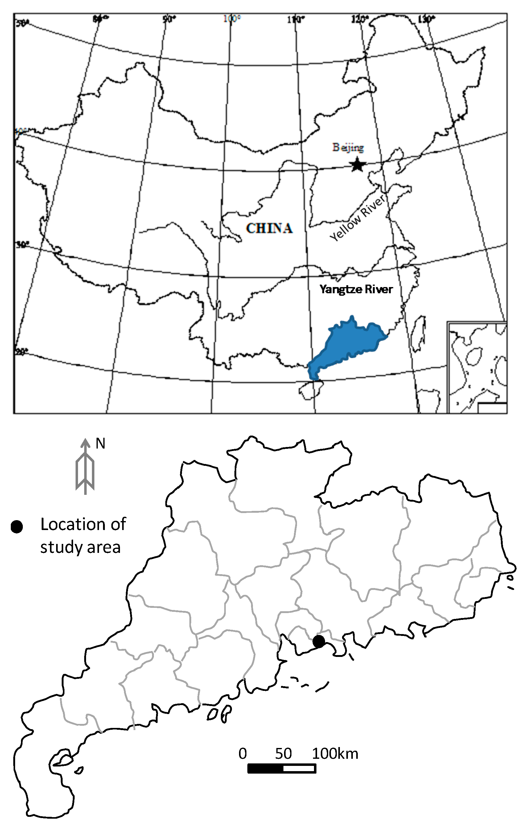
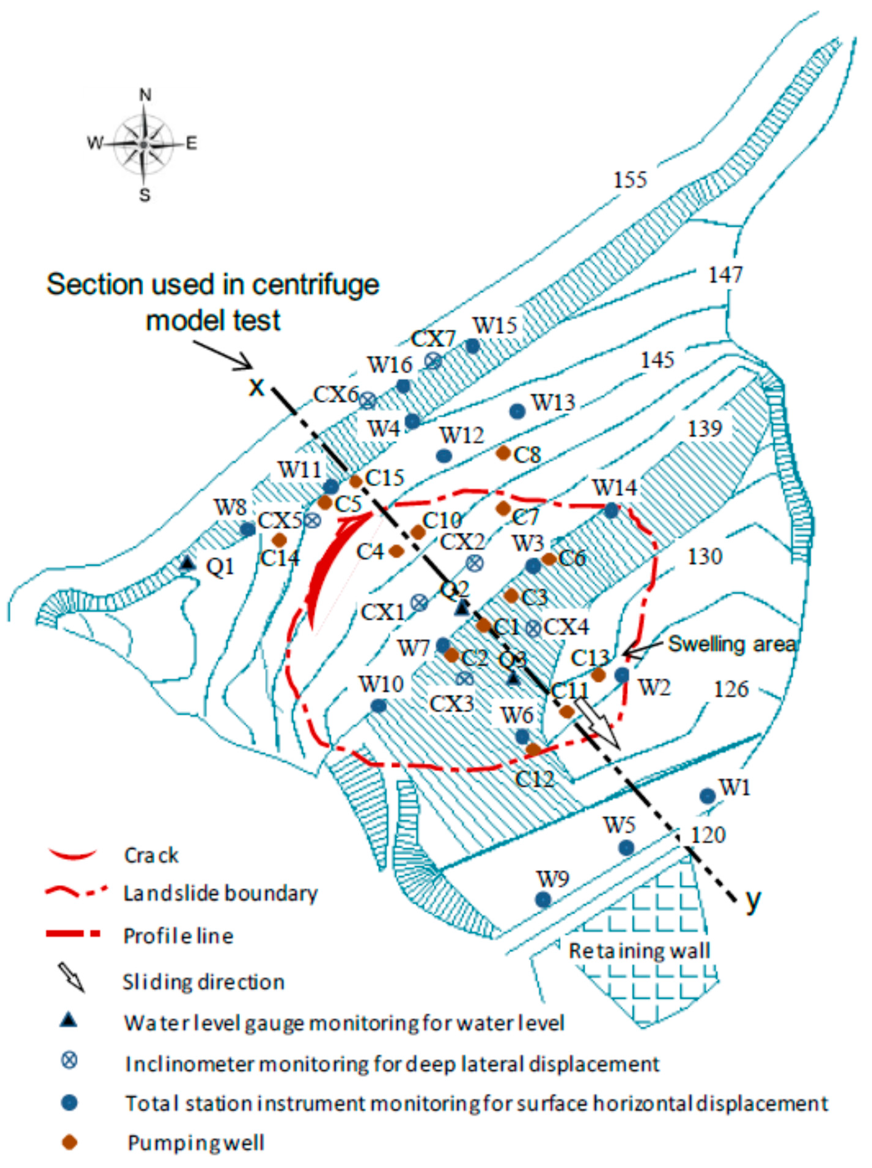
As shown in
Figure 1, the Shenzhen landfill is located in the village of Caopu, Shenzhen City, Guangdong Province, China. It is a typical valley type landfill. The topography at the base of the landfill is in a north to south direction As shown in
Figure 2, a retaining wall was built at the narrow valley end to hold the waste body. Behind the retaining wall in the north-west direction, the slope of the waste body was between 1:3.5 and 1:4. The maximum height of the waste body was about 40 m. At this landsite, the topography varies greatly. On the west side, there is a ridge that extended under the waste body, making the terrain very steep. The slope of the terrain along the base of the waste body was as steep as 24°. The bedrock mainly consists of sandstone (
i.e., siltstone and quartz sandstone). There is no weak intercalated layer or structural plane. The ground is therefore considered a solid foundation.
Figure 1.
Location of the Shenzhen landfill.
Figure 1.
Location of the Shenzhen landfill.
Figure 2.
Site plan of monitoring points and pumping wells.
Figure 2.
Site plan of monitoring points and pumping wells.
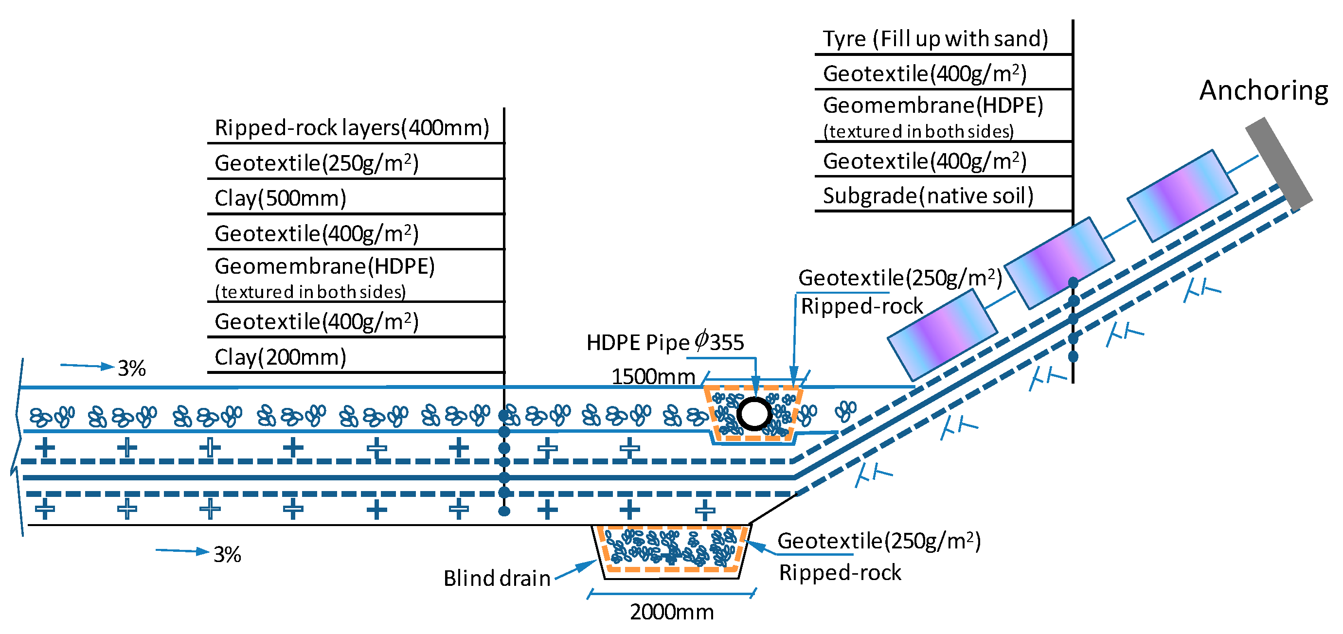
The Shenzhen landfill was one of the earliest sanitary landfills equipped with a composite liner system, as shown in
Figure 3. Based on research results and practical experience, in the composite liner, the shear strength is low at the high-density polyethylene (HDPE) geomembrane/geotextiles and the compacted clay/geotextiles interface [
15]. Hence, these are the weak interfaces for the stability of the waste body.
In 2000, the waste started to accumulate behind the retaining wall. The main components were municipal solid waste and a small amount (<10%) of construction waste. The interim covering layer was clayey soil containing gravel, and the thickness was between 0.5 and 1.0 m. The age of the filled waste ranged between 3 and 10 years, with the oldest waste at the bottom and the youngest at the top.
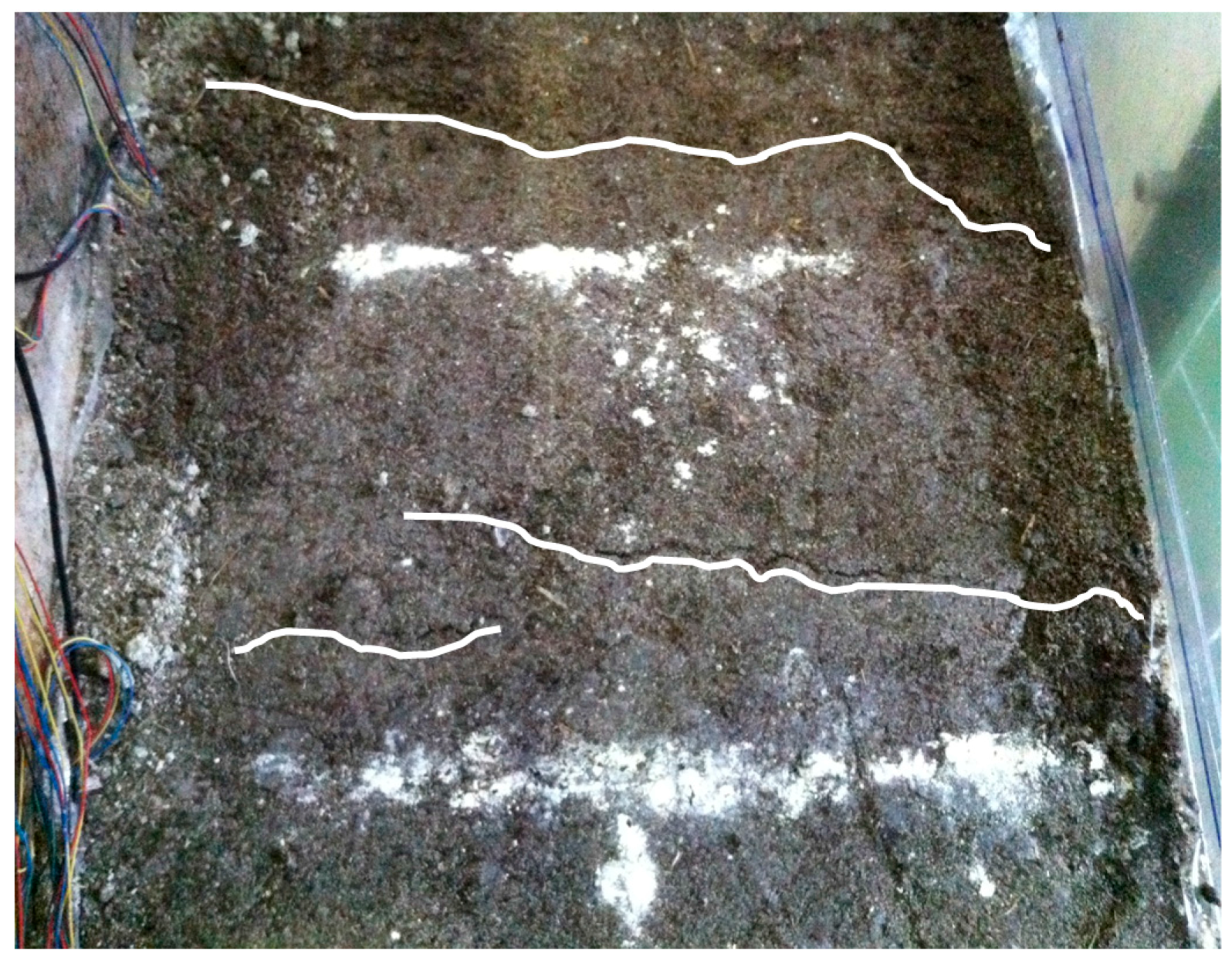
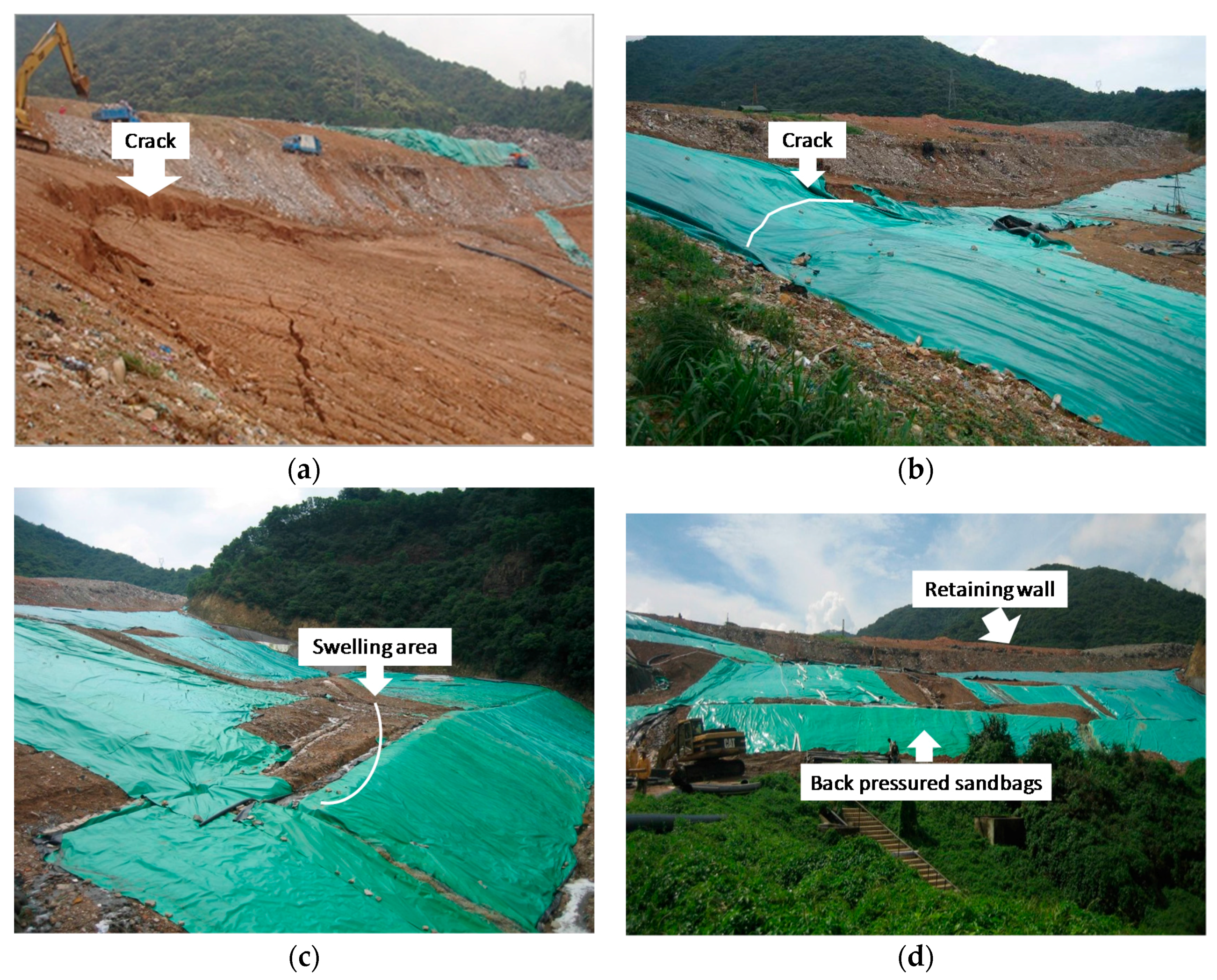
During the heavy rainfall events in 17–18 April 2008, the waste body slid by 1~2 m. The slip area was on the west side, about one-third from the top of the waste body. During another heavy rainfall event in 6–7 June 2008, the middle part and lower part of the waste body slid by 1~4 m. As shown in
Figure 4, due to the slip, a ridge of more than 3 m in height was formed. There was heave in the slip area which extended from one-third to two-thirds from the top of the waste body.
Figure 3.
Structural drawing of the composite liner system.
Figure 3.
Structural drawing of the composite liner system.
Figure 4.
Shenzhen landfill in June 2008 (a) Crack at the trailing edge of waste body; (b) Plastic mulch paved on the waste body surface; (c) Swelling area; (d) Retaining wall.
Figure 4.
Shenzhen landfill in June 2008 (a) Crack at the trailing edge of waste body; (b) Plastic mulch paved on the waste body surface; (c) Swelling area; (d) Retaining wall.
3. Field Monitoring and Emergency Management
According to the field observations, in early March 2008, a crack was formed on the west side near the top of the waste body. As such, that area was in a state of instability. Therefore, the local government decided to monitor the deformation of the landfill slope so that emergency actions could be carried out as necessary. The field monitoring included water level gauges for the monitoring of water levels, electronic total stations for the monitoring surface horizontal displacements, and inclinometers for the monitoring of deep horizontal displacements.
3.1. Monitoring of Water Level
There were a total of 10 water level gauges; three were installed in the water pipes (identified as Q1–Q3 in
Figure 2). The other seven were installed in the inclinometer casing (CX1–CX7 in
Figure 2). The water level was measured using a standpipe piezometer interrogated with a dipmeter.
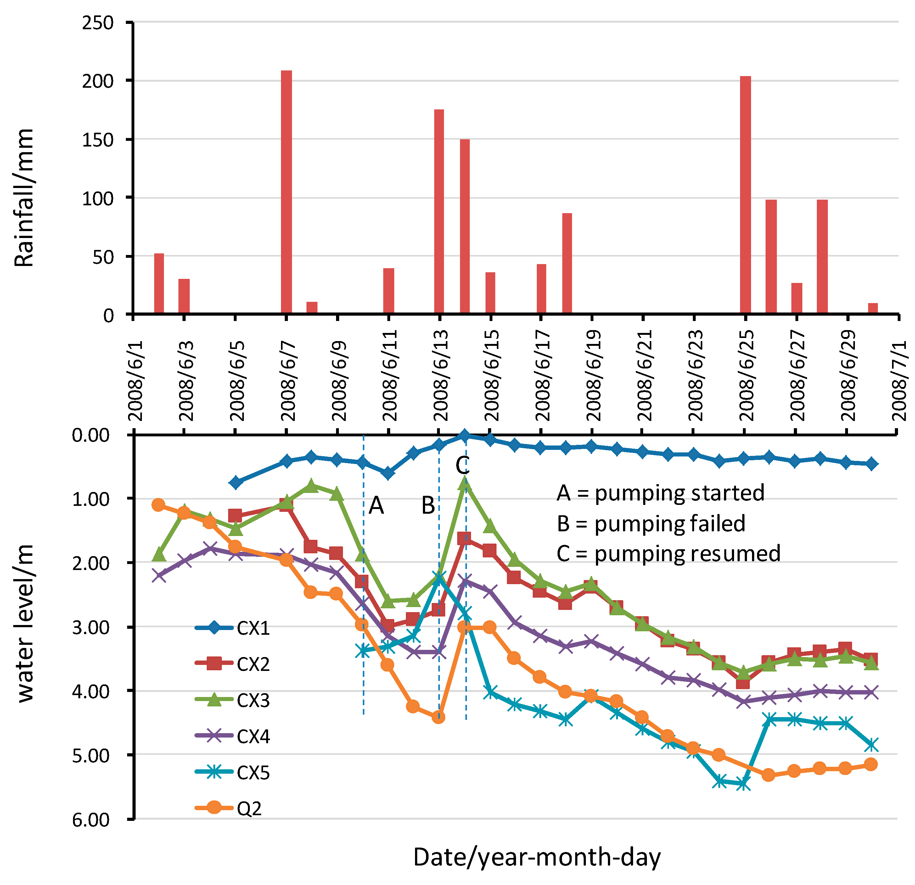
Figure 5 shows some of the monitored water level data and rainfall data in June, 2008. Water depth was measured from the surface of the waste body which was taken as zero. Water level gauges CX2~CX5 and Q2 were within the slip area, which also had dewatering wells during the 2008 emergency. As shown in
Figure 5, the water level within the waste body was very high at the beginning of June, and the water surface was 2 m below the surface of the waste body. It was observed onsite that leachate water mixture overflowed near the retaining wall, which eventually caused the waste body to slide during the 6~7 June heavy rainfall event. On 10 June, the construction of 15 wells within the waste body started, and plastic mulch was paved on the waste body surface so as to reduce infiltration of rainwater into the body. On 13 June, due to heavy rain and the failure of the pumping system, the water level again rose quickly . Subsequently, the pumping resumed and the water level fell quickly. The water levels in gauges CX2~CX5 all dropped to 3.5 m below the surface, and the water level in gauge Q2 dropped to 5.0 m below the surface. Regarding the gauge CX1, it was located in a position where there was a rise in topography. The thickness of the waste body was thin, and due to the supply of leachate and water from upstream, the water level change was not obvious.
Figure 5.
Change of water level with time and rainfall conditions.
Figure 5.
Change of water level with time and rainfall conditions.
3.2. Monitoring of Surface Horizontal Displacement
To capture the state of sliding of the waste body in a timely manner, total station instruments were installed so as to monitor the horizontal surface movements. A total of sixteen (W1–W16) surface displacement monitoring gauges were installed. The gauges W12–W16 were installed for the purpose of monitoring the displacements within the slip zone, which were greater after the 6–7 June heavy rainfall event.
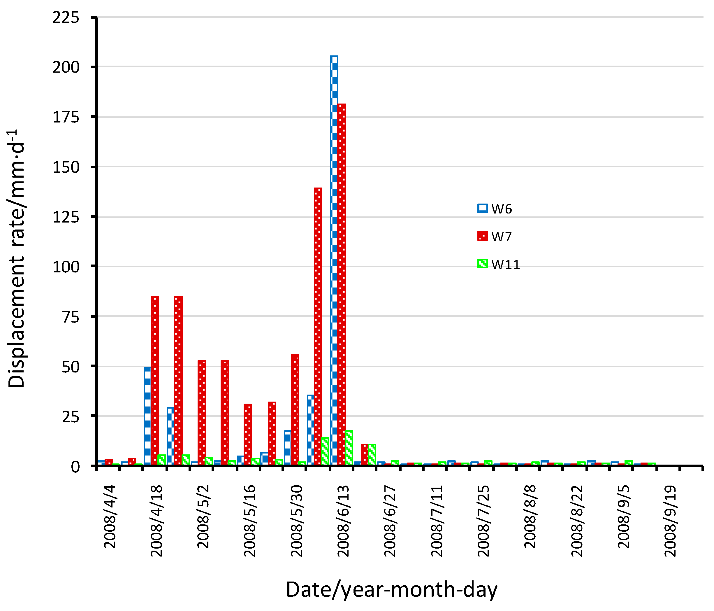
The surface horizontal displacement rate in the waste body is a direct reflection of the landfill movement. As the monitoring frequency varied according to the season and the displacement rate (
Table 1),
Figure 6 shows the adjusted monitored surface horizontal displacement rates from March–October, 2008. Since the recordings of the W6, W7, W11 gauges respectively represent the horizontal surface displacements of the lower, middle and top part the waste body (
Figure 2), only the results from these three gauges are shown in
Figure 6.
Figure 6.
Surface horizontal displacement rates for gauges W6, W7 and W11.
Figure 6.
Surface horizontal displacement rates for gauges W6, W7 and W11.
Table 1.
Horizontal displacement rate and monitoring frequency during dry and rainy seasons.
Table 1.
Horizontal displacement rate and monitoring frequency during dry and rainy seasons.
| Meteorological Condition | Dry Season | Dry Season | Rainy Season | Rainy Season |
|---|
| Horizontal displacement rate (DR) | DR < 5 mm/d | 5 mm/d > DR < 10 mm/d | 5 mm/d > DR < 10 mm/d | DR > 10 mm/d |
| Monitoring frequency | Once a month | Once a week | Once a day | Twice a day |
Considering the rainfall condition in June and the rise in water level, there were increases in the average daily displacement rates for all three gauges. In particular, the large displacement rates in 6–7 June, and 13 June correspond to the two slides. As shown in
Figure 6, the gauge W7 shows that the average daily surface horizontal displacement rates at the centre of the waste body were 135 mm/d and 185 mm/d during the two slides. The average displacement rate in the centre of the waste body is generally greater than that for the rest of the body. The displacement rate of the posterior region in the waste body is also generally smaller. This shows that the gauges W6 and W7 were within the same slip plane, with the centre part of the waste body moving outward.
3.3. Monitoring of Deep Lateral Displacement
At the monitoring point, elevation of the bottom of the landfill and the thickness of the waste can be determined based on geological data. The boreholes could be drilled to the required depth, where the bottom of the boreholes kept a certain distance (ranged from 3 to 5 m) from the liner. Inclinometer casings were then lowered into the borehole, and subsequently these boreholes were backfilled with gravel (3 to 6 mm in grain size). The bottom of the inclinometer casing was not fixed, so both the surface horizontal displacement monitoring and the deep lateral displacement monitoring ought to be carried out simultaneously. In this way, by combining the monitored horizontal displacement at the top of the inclinometer with the monitored lateral displacement at different depths of the inclinometer, the actual displacement at different depths of the waste body can then be derived.
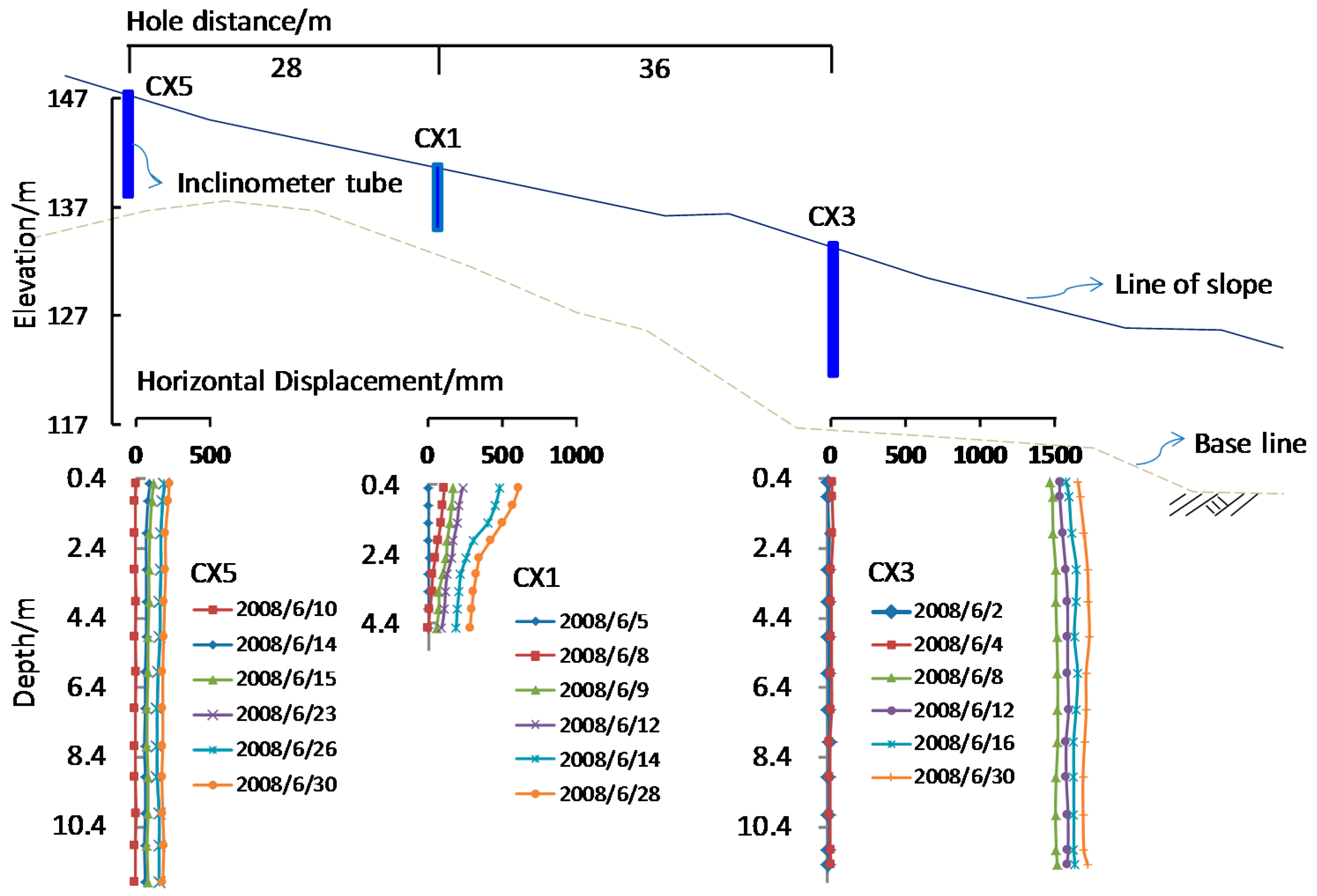
Figure 2 shows the locations of the deep lateral displacement monitor points. Using the monitoring results of gauges CX1, CX3 and CX5,
Figure 7 shows a set of typical monitoring results. These three gauges are in a line parallel to the x–y line. The gauge CX3 was located in the middle of the waste body. The gauge CX1 was located at the bulging area at the lower part of the waste body. The gauge CX5 was located near the top of the waste body.
Figure 7 shows that there was very little displacement at the lower part of the waste body, while there was large displacement in the middle part. The recordings of gauge CX5 show that the displacements are consistent throughout the entire depth of the gauge, where the displacement was as large as 1.5 m on 8 June. At this location, the depth of the sliding waste body was about 12 m. A comparison of the displacement results of the three gauges show that the slip surface went through the middle-lower part of the CX1 inclined tube, but not through the CX5 tube. This result suggests that the deformation occurred at the deep composite liner system. The translational slide is the most likely failure mode.
Figure 7.
Monitored deep lateral displacements at various time.
Figure 7.
Monitored deep lateral displacements at various time.
3.4. Emergency Management
After the landslide, a variety of emergency measures have been carried out, which subsequently proved to be effective. After the 6–7 June heavy rainfall event, 15 pumping wells were drilled into the waste body, as shown in
Figure 2. It can be seen from
Figure 5 that after the start of the pumping, the water level in the wells fell. At the same time, a plastic film was laid on top of the waste body so as to reduce infiltration to the body. Further, the drains were unclogged so that the surface water in concave area could flow out. At the point where the leachate overflowed, the drainage pipe was connected to a gravel ditch so that the leachate could flow out. Finally, sandbags were used to exert a back pressure to the bulging area at the foot of the slope. After these rescue measures, it can be seen from
Figure 6 that the displacement rates of the waste body slowed down significantly. In the subsequent heavy rainfall event, there was no obvious slip. These emergency measures played a key role in preventing further landslide during the 2008 rainy season.
4. Analysis of the Landslide Mechanisms
The use of liner systems for landfill design and construction brings some challenges. Construction of a landfill includes the placement of soil cover and waste layers up to various heights over these liners can result in application of substantial down-slope shear stresses on the liners leading to development of significant liner tension. In addition, interface strengths of the composite liner system may not be enough to resist the increased gravity forces gravity, which resulted in deep sliding along the weak interface at the bottom of landfill.
Jones and Dixon [
16] stated that the design of landfills must consider the stability both within and between elements of a lining system. However, when a liner system is anchored on one side, the displacement of the geosynthetics on that side is then limited. As such, the distribution of forces within each component is complex as it is mainly due to the deformability and frictional interaction between components. Therefore, to use an analytical method to determine the tensile stress in the geomembrane, and the displacement between each interface becomes more difficult. Hence, numerical simulation is often used to simulate the composite liner interface characteristics and the tensile properties of the composite liner [
17,
18,
19,
20,
21]. The explicit difference modelling code, FLAC (Fast Lagrangian Analysis of Continua in 2-Dimensions) (Itasca International Inc., Minnesota, MN, USA) [
22], is the most commonly used numerical analysis technique for simulating landfill lining systems.
Based on the field monitoring data, it can be deduced that the slip is most likely to occur at the side slope. Therefore, FLAC was mainly used to study the characteristics of the composite liner system at the side slope of Shenzhen landfill. In the current study, a three-layer geosynthetic lining system has been analyzed. Beam elements attached to sub-grids on both side with interfaces have been used to represent the geosynthetic elements (Itasca 2007) [
22]. A series of direct shear tests were used to simulate the behavior of the critical interface in the geosynthetic multilayer liner system.
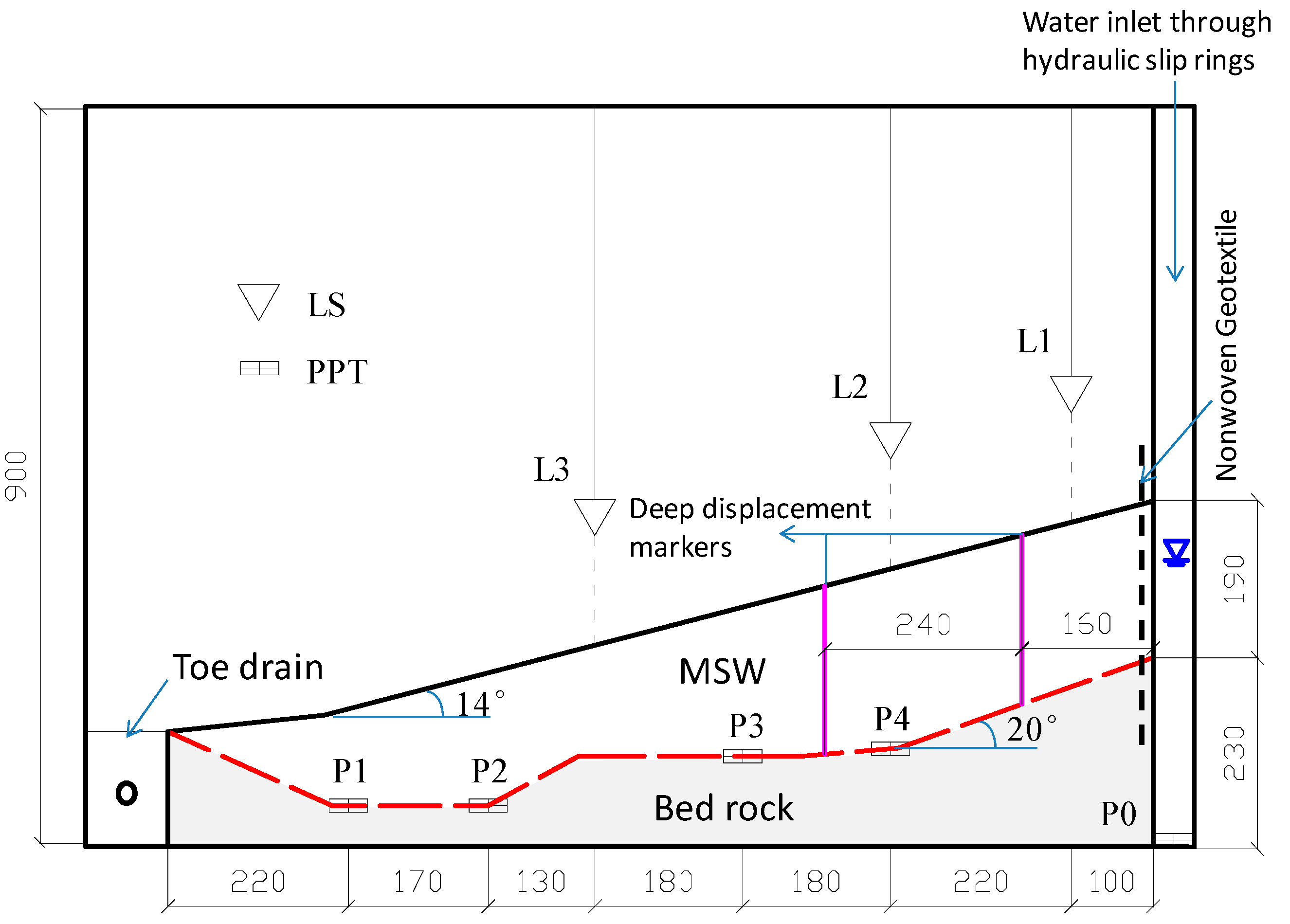
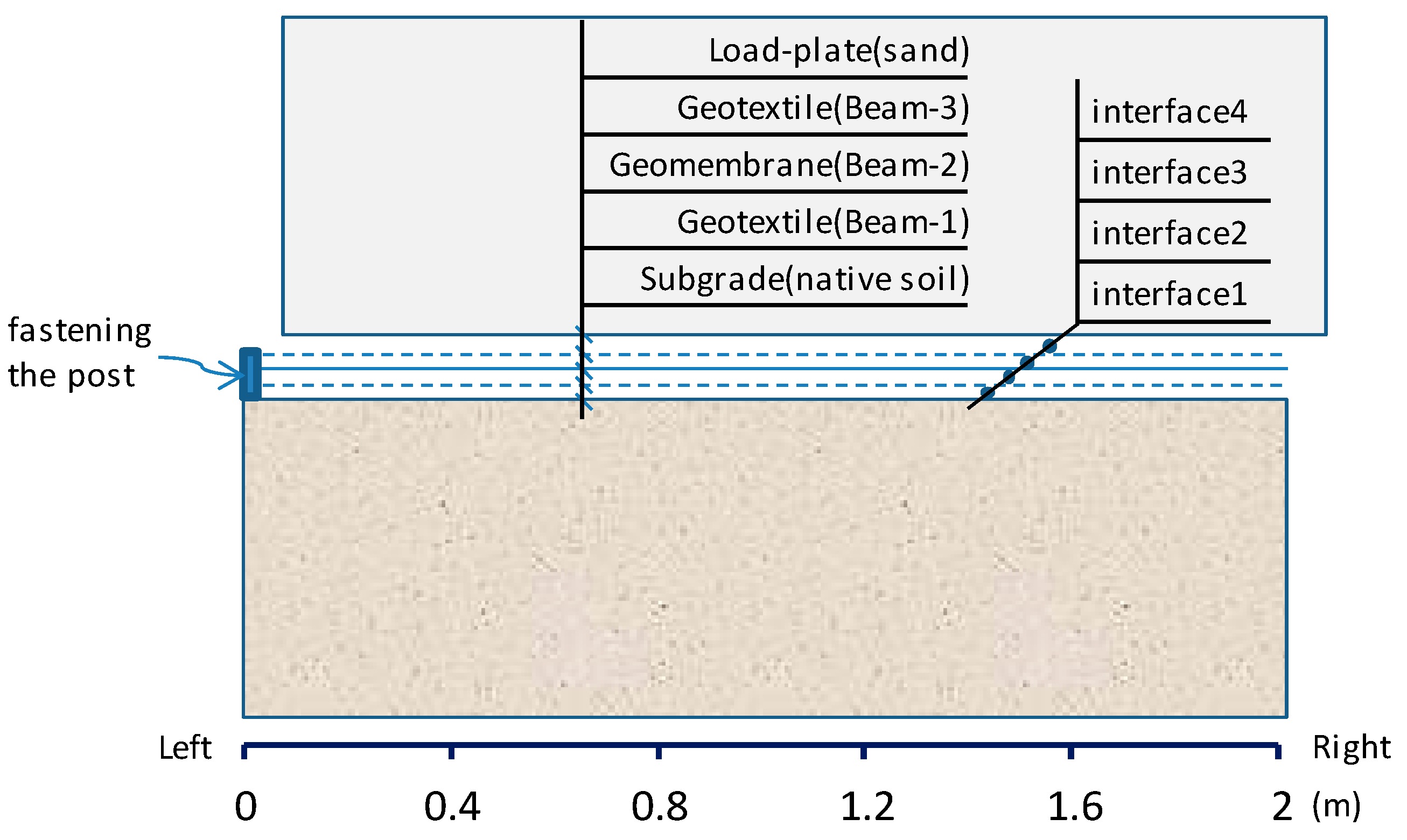
In the simulation model, the length has been set at 2 m. In the model, the left side of the liner system has been fixed so as to simulate the operation condition in the field where the fastening posts were anchored at the top of the slope, as shown in
Figure 8.
Figure 8.
Composite liner system in direct shear test.
Figure 8.
Composite liner system in direct shear test.
The beams were modelled using a linear elastic law. The tensile strength data for the textured HDPE geomembranes (GM) and the geotextiles (GT) were acquired from the laboratory tests, as shown in
Table 2. The interface behavior was assured to be elastic-perfectly with a Mohr-Coulomb failure criterion. The interface parameters resulting from the shear box characterization tests are shown in
Table 3. Villard
et al. [
18] describes the method on how to determine the values of these parameters. The system used, and the results obtained for the GT/GM interface, are shown in
Figure 9. An elastic element with a bulk modulus of 2e5kPa, and a shear modulus of 1e5kPa was used to simulate the load-plate (sand) and subgrade (native soil).
Table 2.
Mechanical properties of geosynthetics (modified from Lin, 2009 [
15]).
Table 2.
Mechanical properties of geosynthetics (modified from Lin, 2009 [15]).
| Geosynthetics | Thickness (mm) | Tensile Stiffness (kN/m) |
|---|
| Textured HDPE geomembrane | 1.5 | 380 |
| Geotextile(400 g/m2) | 4 | 33.3 |
Table 3.
Friction parameters of the various interfaces (modified from Lin, 2009 [
15]).
Table 3.
Friction parameters of the various interfaces (modified from Lin, 2009 [15]).
| Interface | Cohesion (kPa) | Friction Angle (°) | Normal Stiffness (MPa/m) | Shear Stiffness (MPa/m) |
|---|
| Granular soil/GT | 0 | 24 | 70 | 7 |
| GT/GM | 3 | 19.8 | 60 | 6 |
| GT/Native soil | 0 | 25 | 40 | 4 |
Figure 9.
Geotextile-geomembrane friction tests (reproduced from Lin, 2009 [
15]).
Figure 9.
Geotextile-geomembrane friction tests (reproduced from Lin, 2009 [
15]).
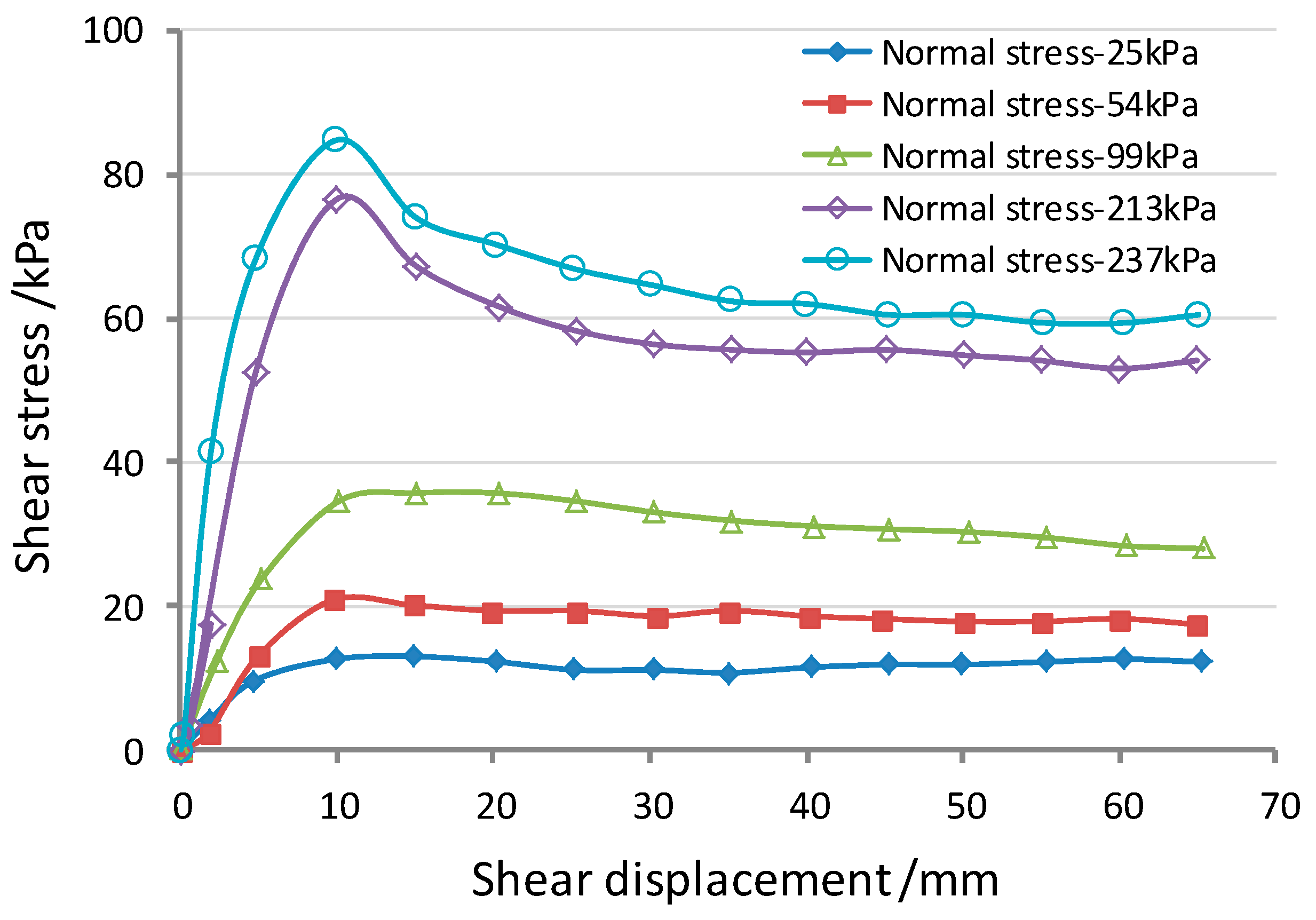
A series of interface tests conducted on a large direct shear apparatus (made by Geotest Company, Shaoxing, China), and the standard used in the test is ASTM (American Society for Testing Material) D5321. Interfaces are given the normal and shear stiffness values, and the interface shear strength.
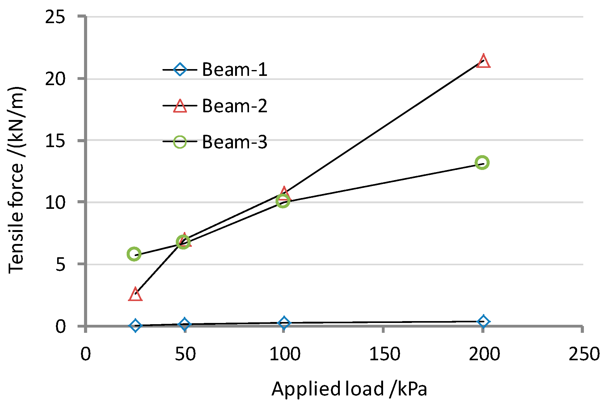
In the simulated direct shear test, a constant shearing speed of 1 mm/min was used together with the normal stresses of 25, 50, 100 and 200 kPa. The tension developed at the beam anchorages in all of the numerical analysis is shown in
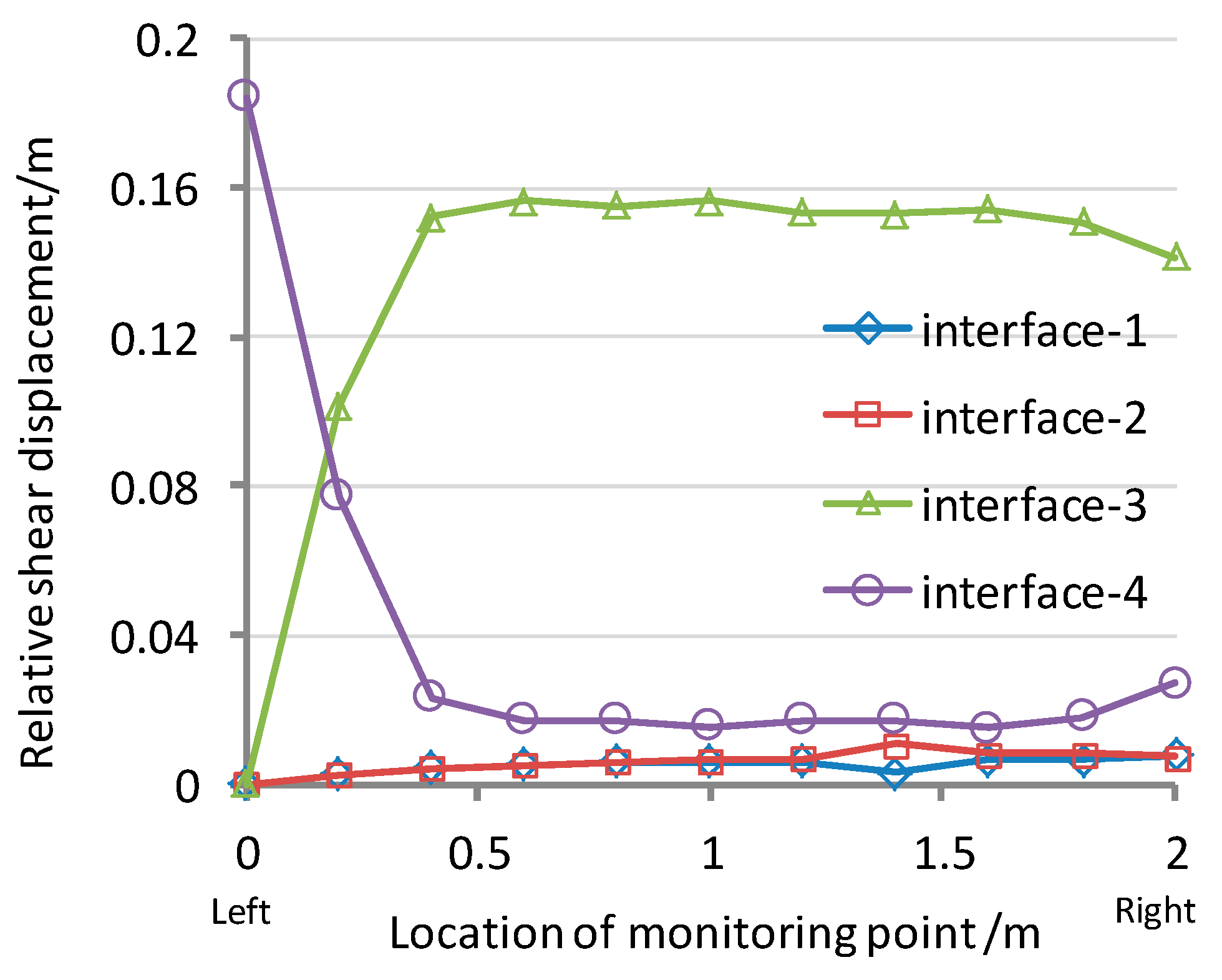
Figure 10. It can be seen that the pulling force of the geosynthetic materials is dependent on the position. The relative shear displacements at the interfaces are shown in
Figure 11. As the peak strength is minimum at the GT/GM interface, the largest relative shear displacements occurred at interface-3, and the displacements measured between the synthetic waste and the geotextile (interface-4) do not reach the post peak values. While the characteristics of interface-2 and interface-3 are similar, but since the GM tensile stiffness is relatively higher, it therefore undertakes a larger shear force coming from the upper part of the composite liner. This limits the relative displacement transferring to interface-2 and interface-1. So, there is only a small tensile stress in the geotextile under the GM, as shown in
Figure 10.
Figure 10.
Tension in the geosynthetic, at anchorage from FLAC models.
Figure 10.
Tension in the geosynthetic, at anchorage from FLAC models.
Figure 11.
Relative interface shear displacements between different interfaces (Normal stress = 100 kPa).
Figure 11.
Relative interface shear displacements between different interfaces (Normal stress = 100 kPa).
According to the results of the numerical models, the trends of the tensile stresses in the geosynthetics and the relative displacements at the interface give the quantitative data. The sliding path within composite liner at the side slope of Shenzhen landfill is most likely to occur between the upper GT/GM interfaces (interface 3).
Therefore, when considering the stability of a landfill which consists of a composite liner layer, it is important to know how much stress is transferred between the interfaces. The weakest interface as well as the most likely slip surface must be identified, so that a reasonable conclusion can be drawn.


