Estimating the Heterogeneous Relationship between Peer Drinking and Youth Alcohol Consumption in Chile Using Propensity Score Stratification

Abstract
:1. Introduction
1.1. An Alternative Statistical Approach: Propensity Score Stratification
1.1.1. Statistical Explanation
1.1.2. Application
1.2. Hypothesis and Analytic Strategy
1.3. Contribution
2. Method
2.1. Data
2.2. Measures
2.2.1. Dependent Variable
2.2.2. Independent and Control Variables
2.2.3. Auxiliary Variables
3. Results and Discussion
3.1. Descriptive Analysis

| Variable | (1) Have Friends Who Drink (n = 631) | (2) No Drinking Friends (n = 283) | p-Value a | ||
|---|---|---|---|---|---|
| Mean (%) | Standard Deviation | Mean (%) | Standard Deviation | ||
| Youth | |||||
| Number of drinks consumed in the past 30 days | 2.27 | 7.90 | 0.07 | 0.29 | <0.001 |
| Male | 50% | -- | 54% | -- | 0.178 |
| Age | 14.79 | 1.47 | 13.49 | 1.05 | <0.001 |
| Family Context | |||||
| Monthly income (unit: 100 Chilean pesos) | 3.19 | 1.60 | 2.98 | 1.45 | 0.056 |
| Less than middle school | 6% | -- | 6% | -- | 0.932 |
| Middle school to less than high school | 35% | -- | 43% | -- | 0.013 |
| High school | 56% | -- | 47% | -- | 0.016 |
| Some college or more | 4% | -- | 4% | -- | 0.933 |
| Married | 65% | -- | 70% | -- | 0.094 |
| Number of drinks consumed in the past 30 days | 16.46 | 44.51 | 15.20 | 39.23 | 0.680 |
| Social Context | |||||
| Neighborhood danger and drugs | 3.11 | 1.07 | 2.77 | 1.12 | <0.001 |
| Advertisement on newspapers/magazines (low exposure) | 23% | -- | 35% | -- | <0.001 |
| Advertisement on newspapers/magazines (moderate exposure) | 39% | -- | 35% | -- | 0.226 |
| Advertisement on newspapers/magazines (high exposure) | 39% | -- | 30% | -- | 0.016 |
| Advertisement on television (low exposure) | 18% | -- | 28% | -- | 0.001 |
| Advertisement on newspapers/magazines (low exposure) | 32% | -- | 31% | -- | 0.894 |
| Advertisement on newspapers/magazines (moderate exposure) | 50% | -- | 41% | -- | 0.007 |
3.2. Negative Binomial Regression under the Homogeneity Assumption
| Variables | Coefficient | Standard Error | Significance |
|---|---|---|---|
| Peers | |||
| Peer alcohol consumption | 2.40 | 0.35 | *** |
| Youth | |||
| Male | 0.40 | 0.23 | † |
| Age | 0.57 | 0.09 | *** |
| Family Context | |||
| Monthly income (unit: 100 Chilean pesos) | −0.47 | 0.29 | |
| Monthly income (squared) | 0.05 | 0.03 | |
| Less than middle school a | 0.04 | 0.73 | |
| Middle school to less than high school a | −0.39 | 0.60 | |
| High school a | −0.39 | 0.59 | |
| Married | −0.04 | 0.25 | |
| Number of drinks consumed in the past 30 days | 0.01 | 0.00 | † |
| Social Context | |||
| Neighborhood danger and drugs | 1.88 | 0.66 | ** |
| Neighborhood danger and drugs (squared) | −0.27 | 0.10 | ** |
| Advertisement on newspapers/magazines (low exposure) b | −0.34 | 0.38 | |
| Advertisement on newspapers/magazines (moderate exposure) b | −0.45 | 0.26 | |
| Advertisement on television (low exposure) c | −0.47 | 0.40 | |
| Advertisement on television (moderate exposure) c | 0.06 | 0.26 | |
| Constant | −12.10 | 1.75 | *** |
3.3. Propensity Score Analysis under the Heterogeneity Assumption
| Variables | Coefficient | Standard Error | Significance |
|---|---|---|---|
| Youth | |||
| Male | −0.11 | 0.10 | |
| Age | 0.46 | 0.04 | *** |
| Family Context | |||
| Monthly income (unit: 100 Chilean pesos) | −0.05 | 0.12 | |
| Monthly income (squared) | 0.01 | 0.01 | |
| Less than middle school a | 0.10 | 0.33 | |
| Middle school to less than high school a | −0.14 | 0.28 | |
| High school a | 0.17 | 0.27 | |
| Married | 0.01 | 0.10 | |
| Number of drinks consumed in the past 30 days | 0.00 | 0.00 | |
| Social Context | |||
| Neighborhood danger and drugs | 0.58 | 0.24 | * |
| Neighborhood danger and drugs (squared) | −0.07 | 0.04 | † |
| Advertisement on newspapers/magazines (low exposure) b | −0.27 | 0.14 | † |
| Advertisement on newspapers/magazines (moderate exposure) b | −0.01 | 0.12 | |
| Advertisement on television (low exposure) c | −0.20 | 0.14 | |
| Advertisement on television (moderate exposure) c | −0.06 | 0.12 | |
| Constant | −6.79 | 0.75 | *** |

| Peer Alcohol Consumption | Stratum 1 | Stratum 2 | Stratum 3 | Stratum 4 | Stratum 5 | ||||||||||
|---|---|---|---|---|---|---|---|---|---|---|---|---|---|---|---|
| Mean | p-Value a | Mean | p-Value a | Mean | p-Value a | Mean | p-Value a | Mean | p-Value a | ||||||
| Yes (n = 38) | No (n = 70) | Yes (n = 84) | No (n = 96) | Yes (n = 80) | No (n = 56) | Yes (n = 129) | No (n = 31) | Yes (n = 300) | No (n = 30) | ||||||
| Youth | |||||||||||||||
| Male | 0.68 | 0.56 | 0.20 | 0.54 | 0.52 | 0.84 | 0.54 | 0.66 | 0.15 | 0.42 | 0.48 | 0.51 | 0.48 | 0.43 | 0.60 |
| Age | 12.35 | 12.40 | 0.59 | 13.27 | 13.22 | 0.65 | 13.93 | 13.85 | 0.34 | 14.35 | 14.43 | 0.45 | 15.95 | 15.21 | 0.00 |
| Family Context | |||||||||||||||
| Monthly income (unit: 100 Chilean pesos) | 2.52 | 2.78 | 0.26 | 3.02 | 3.22 | 0.41 | 3.10 | 2.94 | 0.50 | 3.22 | 2.46 | 0.02 | 3.34 | 3.28 | 0.85 |
| Less than middle school | 0.05 | 0.03 | 0.53 | 0.13 | 0.03 | 0.01 | 0.04 | 0.11 | 0.11 | 0.06 | 0.06 | 0.96 | 0.04 | 0.13 | 0.03 |
| Middle school to less than high school | 0.53 | 0.63 | 0.30 | 0.37 | 0.40 | 0.71 | 0.40 | 0.34 | 0.47 | 0.34 | 0.48 | 0.14 | 0.31 | 0.23 | 0.38 |
| High school | 0.39 | 0.31 | 0.40 | 0.48 | 0.53 | 0.46 | 0.53 | 0.50 | 0.77 | 0.56 | 0.45 | 0.29 | 0.61 | 0.60 | 0.94 |
| Some college or more | 0.03 | 0.03 | 0.95 | 0.02 | 0.04 | 0.51 | 0.04 | 0.05 | 0.65 | 0.04 | 0.00 | 0.27 | 0.04 | 0.03 | 0.86 |
| Married | 0.76 | 0.81 | 0.53 | 0.73 | 0.72 | 0.91 | 0.63 | 0.61 | 0.83 | 0.68 | 0.58 | 0.28 | 0.60 | 0.70 | 0.29 |
| Number of drinks consumed in the past 30 days | 19.68 | 10.60 | 0.06 | 22.08 | 17.00 | 0.52 | 10.31 | 19.75 | 0.11 | 11.60 | 7.65 | 0.43 | 18.21 | 19.47 | 0.90 |
| Social Context | |||||||||||||||
| Neighborhood danger and drugs | 2.48 | 2.40 | 0.71 | 2.75 | 2.78 | 0.82 | 2.80 | 2.93 | 0.51 | 3.03 | 2.95 | 0.68 | 3.41 | 3.13 | 0.16 |
| Advertisement on newspapers/magazines (low exposure) | 0.37 | 0.57 | 0.04 | 0.45 | 0.35 | 0.18 | 0.25 | 0.18 | 0.32 | 0.22 | 0.19 | 0.77 | 0.14 | 0.30 | 0.02 |
| Advertisement on newspapers/magazines (moderate exposure) | 0.37 | 0.24 | 0.17 | 0.31 | 0.34 | 0.63 | 0.36 | 0.45 | 0.33 | 0.37 | 0.42 | 0.63 | 0.43 | 0.33 | 0.32 |
| Advertisement on newspapers/magazines (high exposure) | 0.26 | 0.19 | 0.35 | 0.24 | 0.30 | 0.34 | 0.39 | 0.38 | 0.88 | 0.41 | 0.39 | 0.81 | 0.43 | 0.37 | 0.48 |
| Advertisement on television (low exposure) | 0.34 | 0.43 | 0.38 | 0.26 | 0.32 | 0.37 | 0.16 | 0.21 | 0.44 | 0.24 | 0.10 | 0.08 | 0.12 | 0.13 | 0.83 |
| Advertisement on television (moderate exposure) | 0.24 | 0.27 | 0.70 | 0.39 | 0.30 | 0.20 | 0.36 | 0.36 | 0.95 | 0.26 | 0.29 | 0.76 | 0.31 | 0.37 | 0.55 |
| Advertisement on television (high exposure) | 0.42 | 0.30 | 0.21 | 0.35 | 0.38 | 0.68 | 0.48 | 0.43 | 0.59 | 0.50 | 0.61 | 0.24 | 0.57 | 0.50 | 0.48 |
| Observations (n) | 38 | 70 | -- | 84 | 96 | -- | 80 | 56 | -- | 129 | 31 | -- | 300 | 30 | -- |
| Stratum | Coefficient | Standard Error | p-Value | Significance | Observations |
|---|---|---|---|---|---|
| Level-1 | |||||
| 1 | 1.46 | 1.13 | 0.198 | 108 | |
| 2 | 1.66 | 0.66 | 0.012 | * | 180 |
| 3 | 2.85 | 0.92 | 0.002 | *** | 136 |
| 4 | 2.75 | 0.90 | 0.002 | *** | 160 |
| 5 | 3.36 | 0.70 | 0.000 | *** | 330 |
| Level-2 | |||||
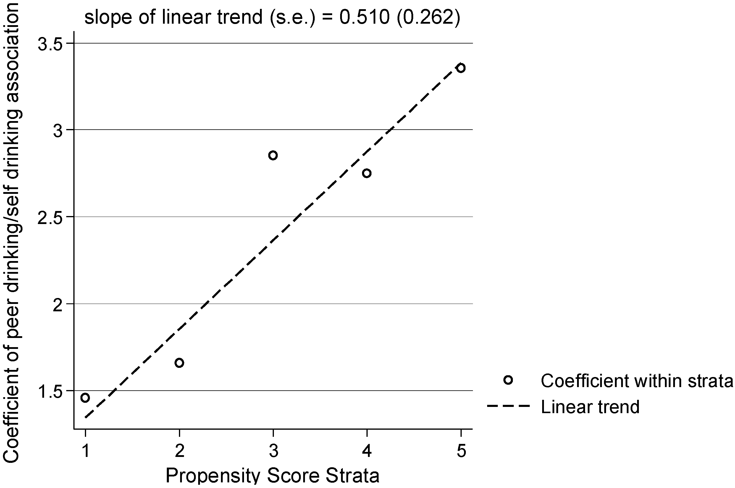
| Slope | 0.51 | 0.26 | 0.052 | † | 914 |
| Constant | 0.83 | 0.91 | 0.361 | ||

| Variables | Stratum 1 | Stratum 2 | Stratum 3 | Stratum 4 | Stratum 5 | (1)–(5) |
|---|---|---|---|---|---|---|
| Mean | Mean | Mean | Mean | Mean | p-Value a | |
| Rule-Breaking | 4.26 | 4.46 | 4.36 | 5.01 | 5.90 | <0.001 |
| Aggression | 6.44 | 7.65 | 7.69 | 9.26 | 8.90 | <0.001 |
| Risk-Taking | 15.61 | 16.16 | 16.59 | 17.03 | 17.71 | <0.001 |
| Self-esteem and Satisfaction | 28.19 | 28.36 | 28.45 | 26.86 | 28.02 | 0.746 |
4. Conclusions
Acknowledgments
Author Contributions
Conflicts of Interest
References
- Thornberry, T.P.; Krohn, M.D. Peers, drug use, and delinquency. In Handbook of Antisocial Behavior; Stoff, D.M., Breiling, J., Maser, J.D., Eds.; J. Wiley & Sons: New York, NY, USA, 1997; pp. 218–233. [Google Scholar]
- Berndt, T.J. Friendship and friends’ influence in adolescence. Curr. Dir. Psychol. Sci. 1992, 1, 156–159. [Google Scholar] [CrossRef]
- Patterson, G.R.; Capaldi, D.; Bank, L. An early starter model for predicting delinquency. In The Development and Treatment of Childhood Aggression; Pelper, D.J., Rubin, K.H., Eds.; Erlbaum: Hillsdale, NJ, USA, 1991; pp. 139–168. [Google Scholar]
- Coleman, J.C.; Hendry, L. The Nature of Adolescence, 3rd ed.; Routledge: London, UK, 1999. [Google Scholar]
- Foster-Clark, F.S.; Blyth, D.A. Peer relations and influences. In Encyclopedia of Adolescence; Lerner, R.M., Petersen, A.C., Brooks-Gunn, J., Eds.; Garland Publisher: New York, NY, USA, 1991; Volume 2, pp. 767–771. [Google Scholar]
- Sieving, R.E.; Perry, C.L.; Williams, C.L. Do friendships change behaviors, or do behaviors change friendships? Examining paths of influence in young adolescents’ alcohol use. J. Adolesc. Health 2000, 26, 27–35. [Google Scholar] [CrossRef] [PubMed]
- Fisher, L.A.; Bauman, K.E. Influence and selection in the friend-adolescent relationship—Findings from studies of adolescent smoking and drinking. J. Appl. Soc. Psychol. 1988, 18, 289–314. [Google Scholar] [CrossRef]
- Urberg, K.A.; DeÄŸirmencioÄŸlu, S.M.; Pilgrim, C. Close friend and group influence on adolescent cigarette smoking and alcohol use. Dev. Psychol. 1997, 33, 834–844. [Google Scholar] [CrossRef] [PubMed]
- Mason, W.A.; Windle, M. Family, religious, school and peer influences on adolescent alcohol use: A longitudinal study. J. Stud. Alcohol 2001, 62, 44–53. [Google Scholar] [PubMed]
- Gardner, T.W.; Dishion, T.J.; Connell, A.M. Adolescent self-regulation as resilience: Resistance to antisocial behavior within the deviant peer context. J. Abnorm. Child Psychol. 2008, 36, 273–284. [Google Scholar] [CrossRef] [PubMed]
- Fergus, S.; Zimmerman, M.A. Adolescent resilience: A framework for understanding healthy development in the face of risk. Annu. Rev. Pub. Health 2005, 26, 399–419. [Google Scholar] [CrossRef]
- Griffin, K.W.; Botvin, G.J.; Scheier, L.M.; Doyle, M.M.; Williams, C. Common predictors of cigarette smoking, alcohol use, aggression, and delinquency among inner-city minority youth. Addict. Behav. 2003, 28, 1141–1148. [Google Scholar] [CrossRef] [PubMed]
- Rosenbaum, P.R.; Rubin, D.B. The central role of the propensity score in observational studies for causal effects. Biometrika 1983, 70, 41–55. [Google Scholar] [CrossRef]
- Rubin, D.B. Estimating causal effects from large data sets using propensity scores. Ann. Intern. Med. 1997, 127, 757–763. [Google Scholar] [CrossRef] [PubMed]
- Xie, Y. Causal inference and heterogeneity bias in social science. Inf. Knowl. Syst. Manag. 2011, 10, 279–289. [Google Scholar]
- Brand, J.E.; Xie, Y. Who benefits most from college? Evidence for negative selection in heterogeneous economic returns to higher education. Am. Sociol. Rev. 2010, 75, 273–302. [Google Scholar] [CrossRef] [PubMed]
- Rosenbaum, P.R.; Rubin, D.B. Reducing bias in observational studies using subclassification on the propensity score. J. Am. Stat. Assoc. 1984, 79, 516–524. [Google Scholar] [CrossRef]
- Kandel, D.B. Homophily, selection, and socialization in adolescent friendships. Am. J. Sociol. 1978, 84, 427–436. [Google Scholar] [CrossRef]
- Hawkins, J.D.; Catalano, R.F.; Miller, J.Y. Risk and protective factors for alcohol and other drug problems in adolescence and early adulthood—Implications for substance-abuse prevention. Psychol. Bull. 1992, 112, 64–105. [Google Scholar] [CrossRef] [PubMed]
- Li, F.Z.; Barrera, M.; Hops, H.; Fisher, K.J. The longitudinal influence of peers on the development of alcohol use in late adolescence: A growth mixture analysis. J. Behav. Med. 2002, 25, 293–315. [Google Scholar] [CrossRef] [PubMed]
- Dodge, K.A.; Dishion, T.J.; Lansford, J.E. The problem of deviant peer influences in intervention programs. In Deviant Peer Influences in Programs for Youth; Dodge, K.A., Dishion, T.J., Lansford, J.E., Eds.; Guilford Press: New York, NY, USA, 2006. [Google Scholar]
- Simons, R.L.; Chao, W.; Conger, R.D.; Elder, G.H. Quality of parenting as mediator of the effect of childhood defiance on adolescent friendship choices and delinquency: A growth curve analysis. J. Marriage Fam. 2001, 63, 63–79. [Google Scholar] [CrossRef]
- Patterson, G.R.; Dishion, T.J.; Yoerger, K. Adolescent growth in new forms of problem behavior: Macro- and micro-peer dynamics. Prev. Sci. 2000, 1, 3–13. [Google Scholar] [CrossRef] [PubMed]
- Hawkins, J.D. Delinquency and Crime: Current Theories; Cambridge University Press: Cambridge, UK, 1999. [Google Scholar]
- Dehejia, R.H.; Wahba, S. Causal effects in nonexperimental studies: Reevaluating the evaluation of training programs. J. Am. Stat. Assoc. 1999, 94, 1053–1062. [Google Scholar] [CrossRef]
- Xie, Y.; Wu, X. Reply: Market premium, social process, and statisticism. Am. Sociol. Rev. 2005, 70, 865–870. [Google Scholar] [CrossRef]
- Caris, L.; Wagner, F.A.; Rios-Bedoyae, C.F.; Anthony, J.C. Opportunities to use drugs and stages of drug involvement outside the United States: Evidence from the Republic of Chile. Drug Alcohol Depend. 2009, 102, 30–34. [Google Scholar] [CrossRef]
- Fuentealba, R.; Cumsille, F.; Araneda, J.C.; Molina, C. Consumption of licit and illicit drugs in Chile: results of the 1998 study and comparison with the 1994 and 1996 studies. Pan Am. J. Pub. Health 2000, 7, 79–87. [Google Scholar] [CrossRef]
- Smetana, J.G.; Campione-Barr, N.; Metzger, A. Adolescent development in interpersonal and societal contexts. Annu. Rev. Psychol. 2006, 57, 255–284. [Google Scholar] [CrossRef] [PubMed]
- Lozoff, B.; de Andraca, I.; Castillo, M.; Smith, J.B.; Walter, T.; Pino, P. Behavioral and developmental effects of preventing iron-deficiency anemia in healthy full-term infants. Pediatrics 2003, 112, 846–849. [Google Scholar] [PubMed]
- Achenbach, T.M.; Rescorla, L. Manual for the ASEBA School-Age Forms & Profiles; ASEBA: Burlington, VT, USA, 2001. [Google Scholar]
- Starfield, B.; Ensminger, M.; Riley, A.; McGauhey, P.; Skinner, A.; Kim, S.; Bergner, M.; Ryan, S.; Green, B. Adolescent health status measurement: Development of the child health and illness profile. Pediatrics 1993, 91, 430–435. [Google Scholar] [PubMed]
- Dishion, T.J.; Owen, L.D. A longitudinal analysis of friendships and substance use: Bidirectional influence from adolescence to adulthood. Dev. Psychol. 2002, 38, 480–491. [Google Scholar] [CrossRef] [PubMed]
- Chartier, K.G.; Hesselbrock, M.N.; Hesselbrock, V.M. Development and vulnerability factors in adolescent alcohol use. Child Adolesc. Psychiatr. Clin. N. Am. 2010, 19, 493–504. [Google Scholar] [CrossRef] [PubMed]
- Dishion, T.J.; Andrews, D.W.; Crosby, L. Antisocial boys and their friends in early adolescence: Relationship characteristics, quality, and interactional process. Child Dev. 1995, 66, 139–151. [Google Scholar] [CrossRef] [PubMed]
- Delva, J.; Han, Y.; Sanchez, N.; Andrade, F.H.; Sanhueza, G.; Krentzman, A. Spirituality and alcohol consumption among adolescents in Chile: Results of propensity score stratification analyses. In Soc. Work Res.; in press.
- Xie, Y.; Brand, J.E.; Jann, B. Estimating heterogeneous treatment effects with observational data. Sociol. Methodol. 2012, 42, 314–347. [Google Scholar] [CrossRef] [PubMed]
© 2014 by the authors; licensee MDPI, Basel, Switzerland. This article is an open access article distributed under the terms and conditions of the Creative Commons Attribution license (http://creativecommons.org/licenses/by/4.0/).
Share and Cite
Han, Y.; Grogan-Kaylor, A.; Delva, J.; Xie, Y. Estimating the Heterogeneous Relationship between Peer Drinking and Youth Alcohol Consumption in Chile Using Propensity Score Stratification. Int. J. Environ. Res. Public Health 2014, 11, 11879-11897. https://doi.org/10.3390/ijerph111111879
Han Y, Grogan-Kaylor A, Delva J, Xie Y. Estimating the Heterogeneous Relationship between Peer Drinking and Youth Alcohol Consumption in Chile Using Propensity Score Stratification. International Journal of Environmental Research and Public Health. 2014; 11(11):11879-11897. https://doi.org/10.3390/ijerph111111879
Chicago/Turabian StyleHan, Yoonsun, Andrew Grogan-Kaylor, Jorge Delva, and Yu Xie. 2014. "Estimating the Heterogeneous Relationship between Peer Drinking and Youth Alcohol Consumption in Chile Using Propensity Score Stratification" International Journal of Environmental Research and Public Health 11, no. 11: 11879-11897. https://doi.org/10.3390/ijerph111111879
APA StyleHan, Y., Grogan-Kaylor, A., Delva, J., & Xie, Y. (2014). Estimating the Heterogeneous Relationship between Peer Drinking and Youth Alcohol Consumption in Chile Using Propensity Score Stratification. International Journal of Environmental Research and Public Health, 11(11), 11879-11897. https://doi.org/10.3390/ijerph111111879