
Machine Learning Applications to Land and Structure Valuation


Abstract
:1. Introduction
2. Methodology
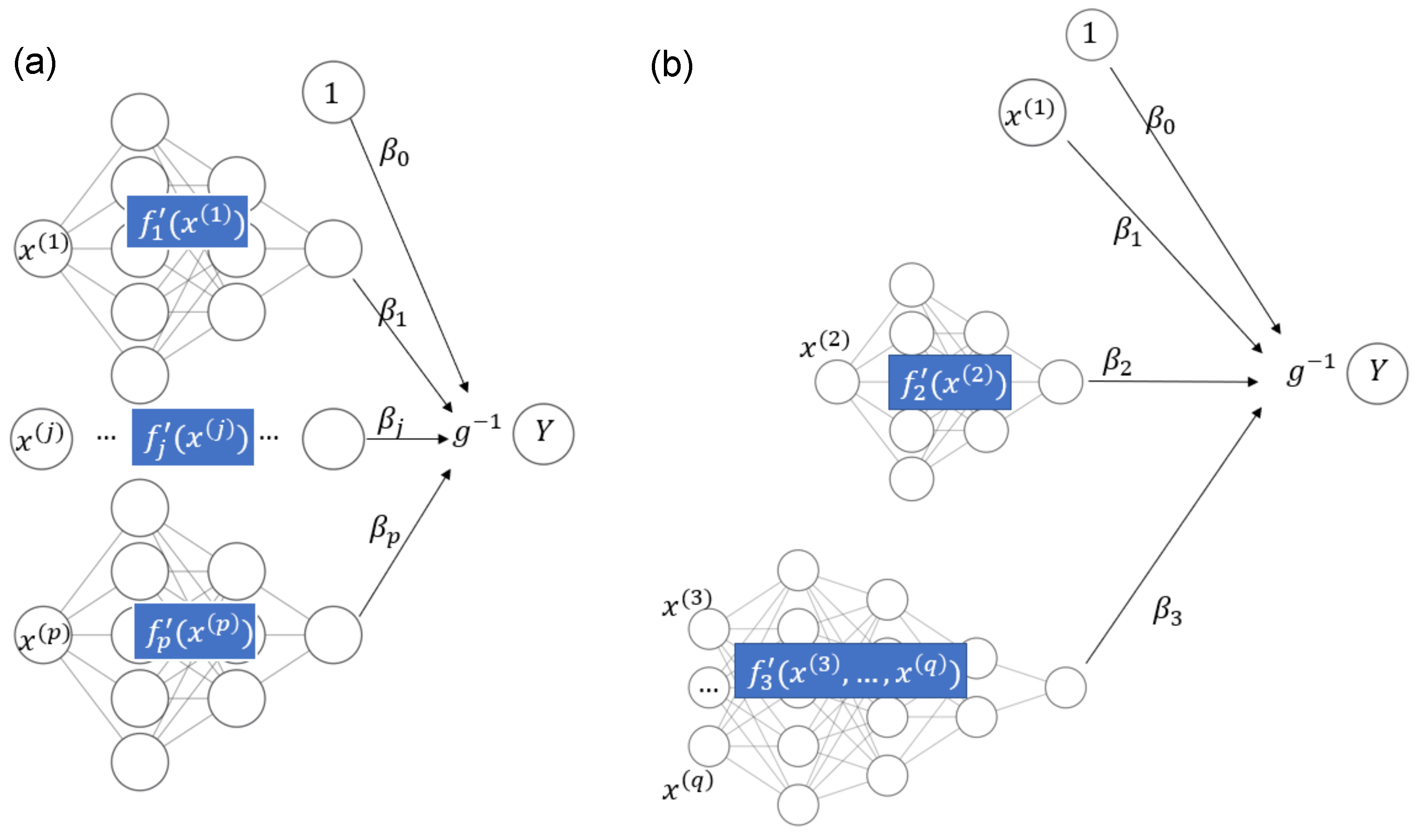
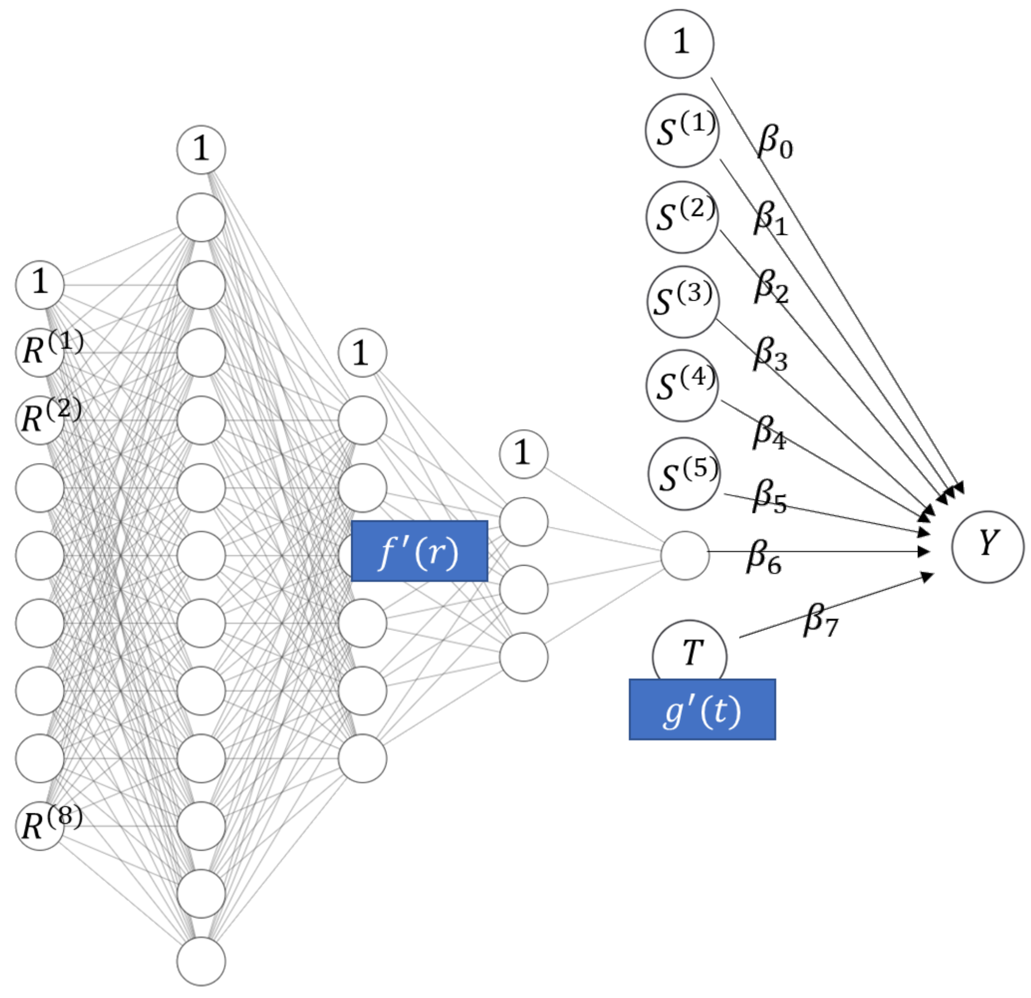
2.1. STAR Models and Deep Learning
2.2. STAR Models and Gradient Boosting
- At the time of writing and until at least XGBoost version 1.4.1.1, XGBoost respects only non-overlapping interaction constraint sets , i.e., partitions. LightGBM can also deal with overlapping constraint sets.
- Boosted trees with interaction constraints support only non-linear components, unlike, e.g., deep learning and component-wise boosting, both of which allow a mix of linear and non-linear components. See Remark 4, as well as our two case studies, for a two-step procedure that would linearize some effects fitted by XGBoost or LightGBM, thus overcoming this limitation.
- Feature pre-processing for boosted trees is simpler than for other modeling techniques. Missing values are allowed for most implementations, feature outliers are unproblematic, and some implementations (including LightGBM) can directly deal with unordered categorical variables. Furthermore, highly correlated features are only problematic for interpretation, not for model fitting.
- Model-based boosting “mboost” with trees as building blocks is an alternative to using XGBoost or LightGBM with interaction constraints.
2.3. STAR Models and Supervised Dimension Reduction
- 1.
- House price models with additive effects for structural characteristics and time (for maximal interpretability) and one multivariate component using all locational variables with complex interactions (for maximal predictive performance). The model equation could be as follows:Component provides a one-dimensional representation of all locational variables. We will see an example of such a model in the Florida case study.
- 2.
- This is similar to the first example, but adding the date of sale to the component with all locational variables, leading to a model with time-dependent location effects. The component depending on locational variables and time represents those variables by a one-dimensional function. Such a model will be shown in the Swiss case study below.
- From the above definition, it directly follows that the purely additive contribution of a (possibly large) set of features provides a supervised one-dimensional representation of the features in , optimized for predictions on the scale of ξ and conditional on the effects of other features.
- For simplicity, we assume that each model component is irreducible, i.e., it uses only as many features as necessary. In particular, a component additive in its features would be represented by multiple components instead.
- The encoder of is defined up to a shift, i.e., for any constant c is an encoder of as well. If c is chosen so that the average value of the encoder is 0 on some reference dataset, e.g., the training dataset, we speak of a centered encoder.
- 1.
- Let . Then,is a purely additive contribution of .
- 2.
- Due to interaction effects, the singleton and are not encodable.
- 3.
- Let and . Then,is an encoder of .
- 4.
- The fitted model is an encoder of the set of all features. This is true for STAR models in general.
| Algorithm 1 Encoder extraction |
|
2.4. Interpreting STAR Models
- To benefit from additivity, effects of features in STAR models are typically interpreted on the scale of ξ.
- ICE profiles and the PDP can be used to interpret effects of non-encodable feature sets as well. Due to interaction effects, however, a single ICE profile or a PDP cannot give a complete picture of such an effect.
- In this paper, we describe feature effects by ICE/PDP/encoders. For alternatives, see Molnar (2019) or Biecek and Burzykowski (2021).
- The administrative unit (a one-dimensional feature).
- The address (also a one-dimensional feature).
- Latitude/longitude (a two-dimensional feature).
3. Case Study 1: Miami Housing Data
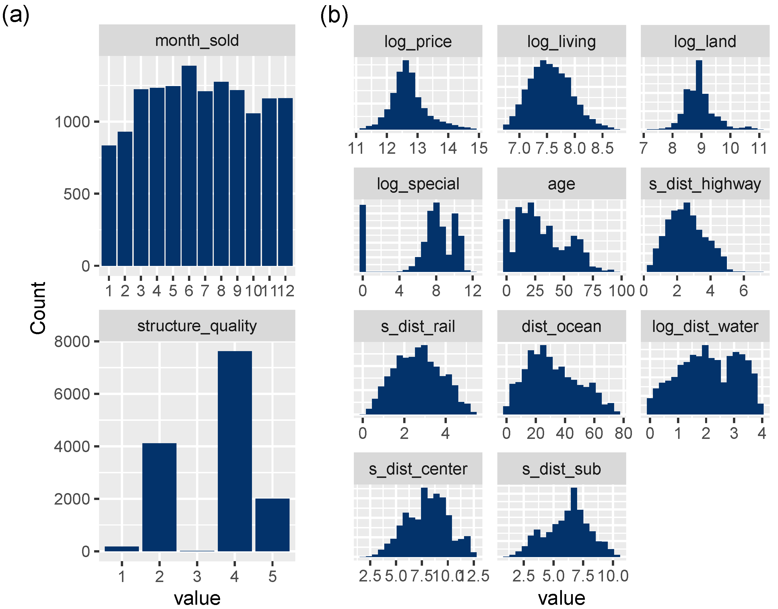
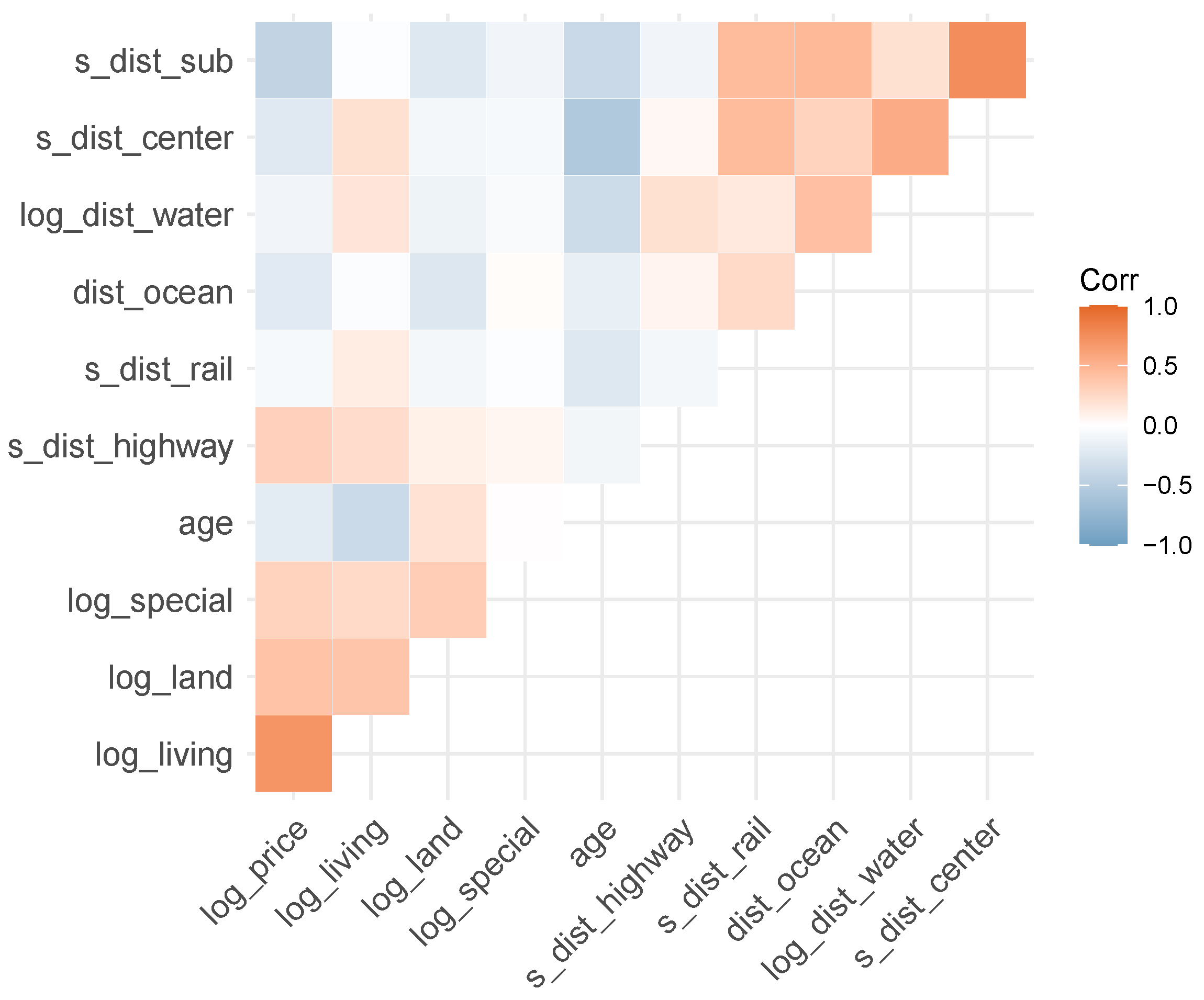
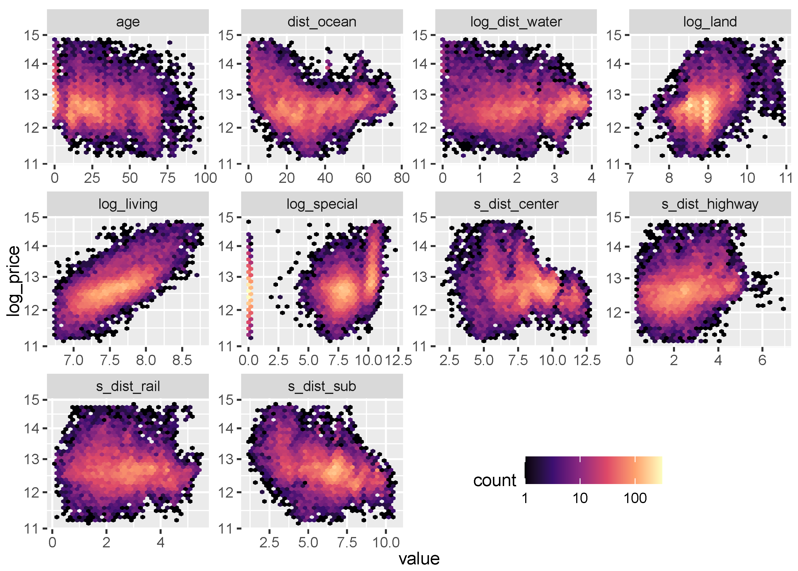
3.1. Data
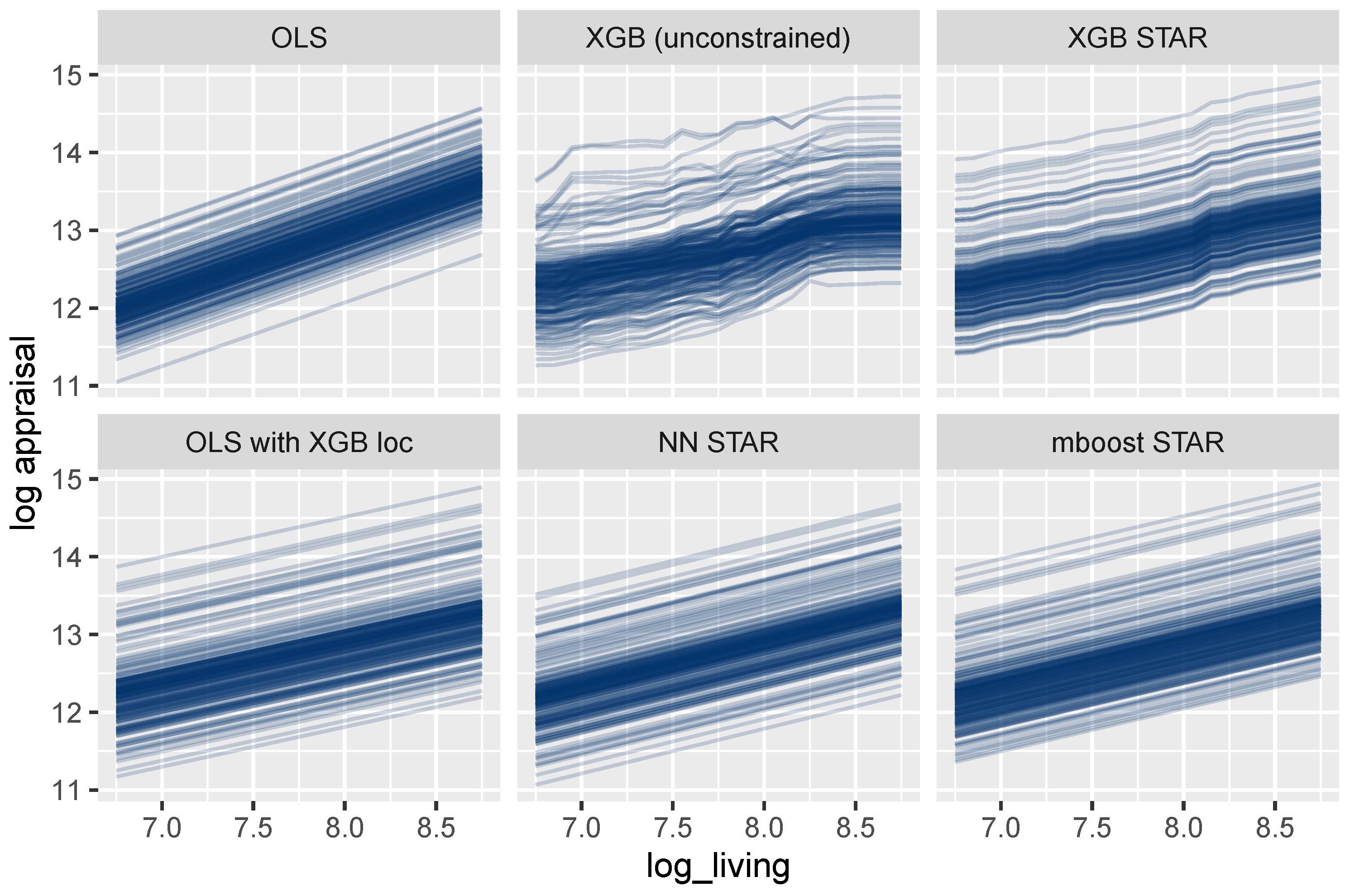
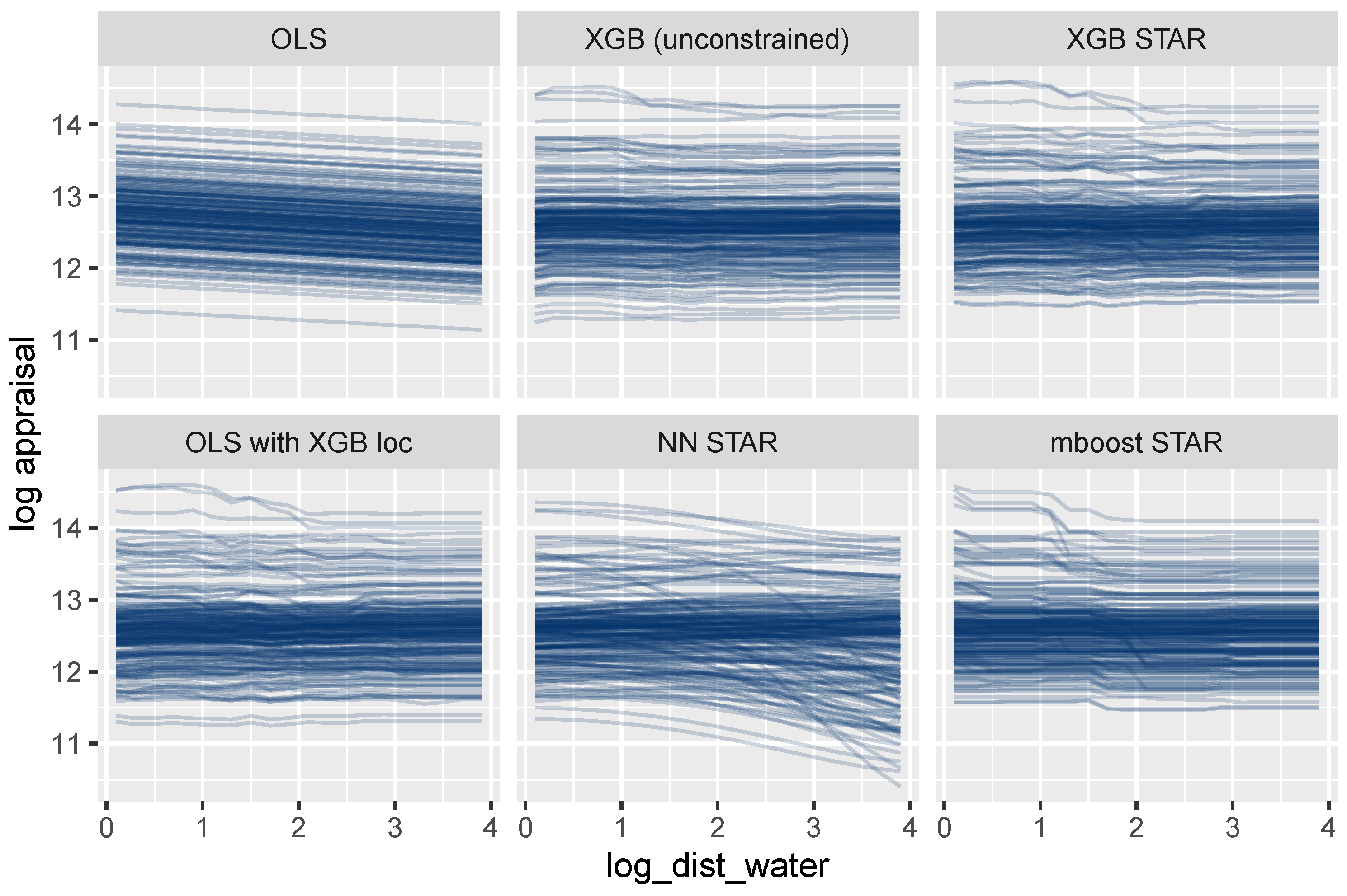
3.2. Models
- OLS: Linear regression benchmark with maximal interpretability.
- XGB (unconstrained): XGBoost benchmark for maximal performance.
- XGB STAR: XGBoost STAR model for high interpretability and performance.
- OLS with XGB loc: Linear model with location effects derived from XGB STAR.
- NN STAR: Deep neural STAR model.
- mboost STAR: mboost STAR model.
3.3. Results
3.3.1. Performance
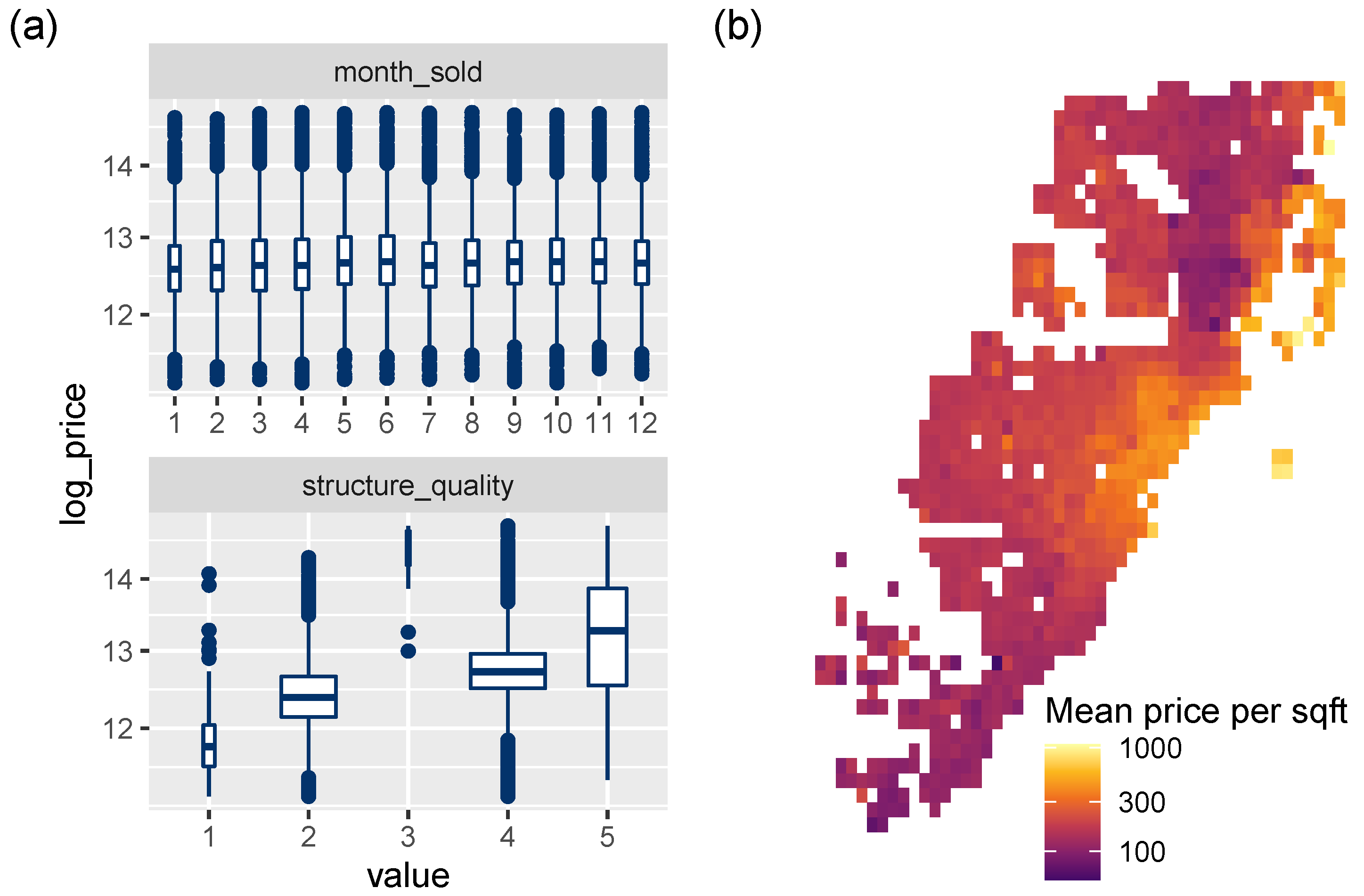
3.3.2. Effects of Single Variables
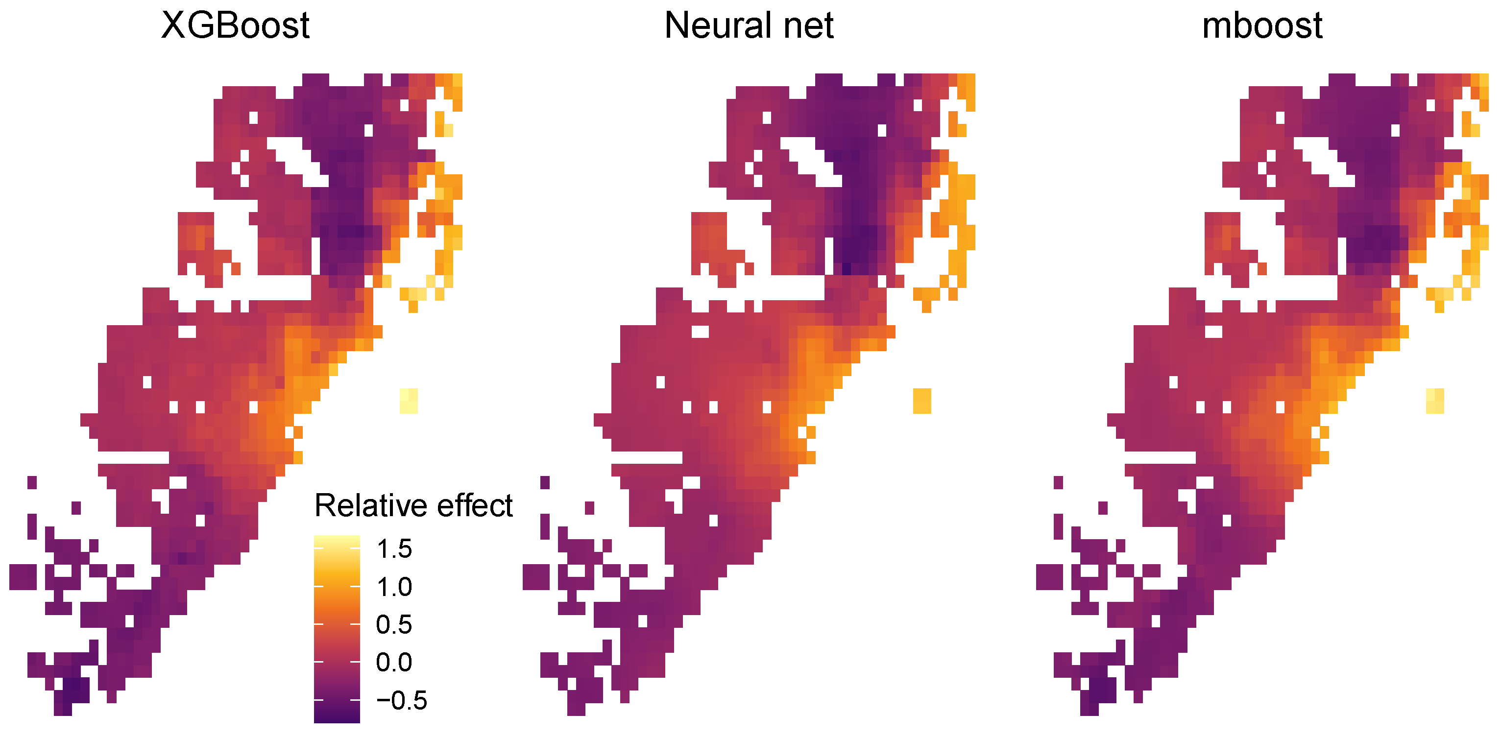
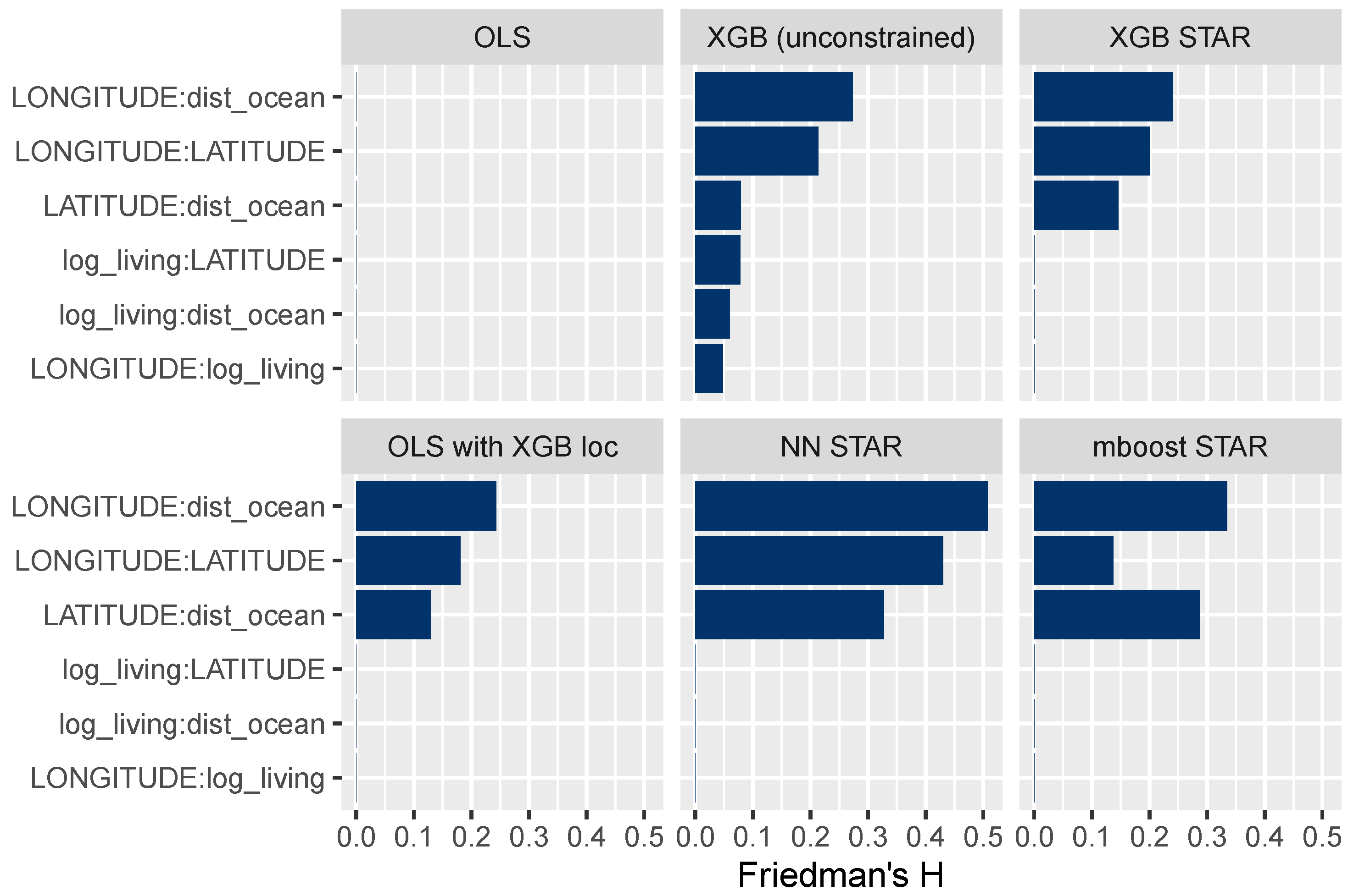
3.3.3. Interaction Effects
3.3.4. Supervised Dimension Reduction and Location Effects
4. Case Study 2: Swiss Housing Data
4.1. Data
- Twelve pre-transformed property characteristics (logarithmic living area, number of rooms, age, etc.) represented by the feature vector .
- Transaction time (year and quarter) T.
- A set of 25 untransformed locational variables mostly available at the municipal level, such as the average taxable income or the vacancy rate.
- Latitude and longitude.
- For 25 points of interest (POIs), such as schools, shops, or public transport, their individual counts within a 500 m buffer.
- The distance from the nearest POI of each type to the house (maximum 500 ).
4.2. Models
- LGB (unconstrained): LightGBM benchmark for maximum performance. Hyper-parameter tuning was done by stratified five-fold cross-validation, using a learning rate of 0.1 and systematically varying the number of leaves, row and column subsampling rates, and L1 and L2 penalization. As for the XGBoost models in the first case study, the number of trees (1918) was chosen by early stopping on the cross-validation score. The model was fitted with the R package lightgbm (Ke et al. 2021), using the absolute error loss in order to provide a model for the conditional median (Table 2).
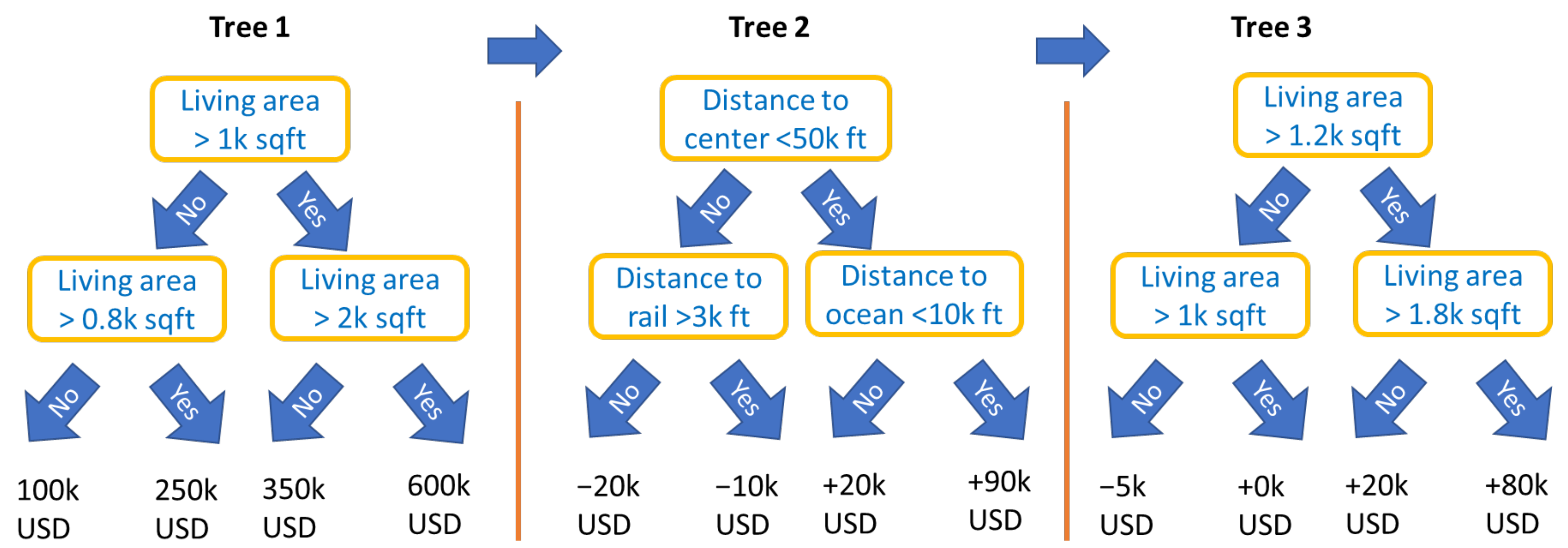
- LGB STAR: LightGBM STAR model for high interpretability and performance. This is built similarly to the first model (with 2225 trees), but with additive effects for building variables enforced by interaction constraints. Locational variables and transaction time were allowed to interact with each other. This leads to a model of the form
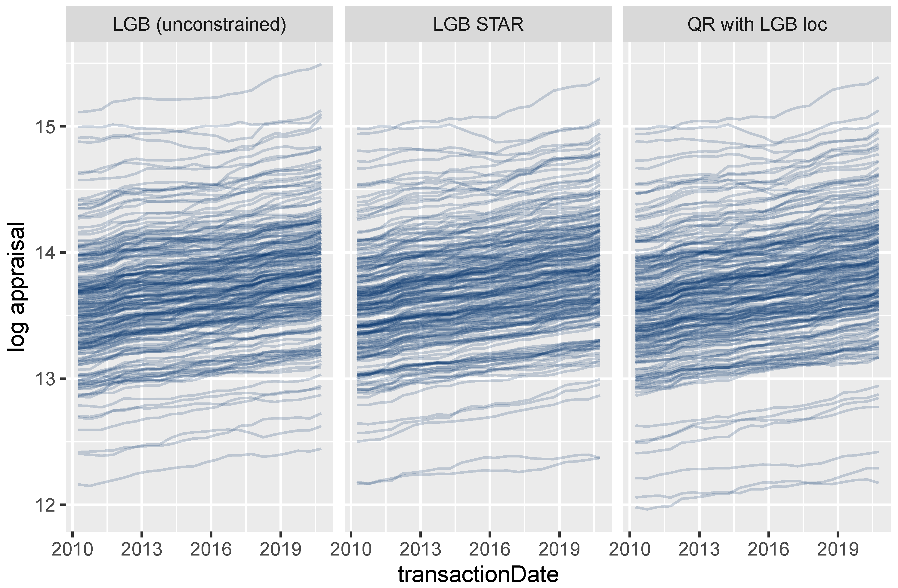
- QR with LGB loc: Linear quantile regression (Koenker 2005) with time-dependent location effects derived from LGB STAR model, using Algorithm 1 to extract the centered encoder . The model equation is thusand can be viewed as a linearized LightGBM quantile regression model. The model was fitted with the R package quantreg (Koenker 2021).
4.3. Results
4.3.1. Performance
4.3.2. Effects of Additive and Non-Additive Features
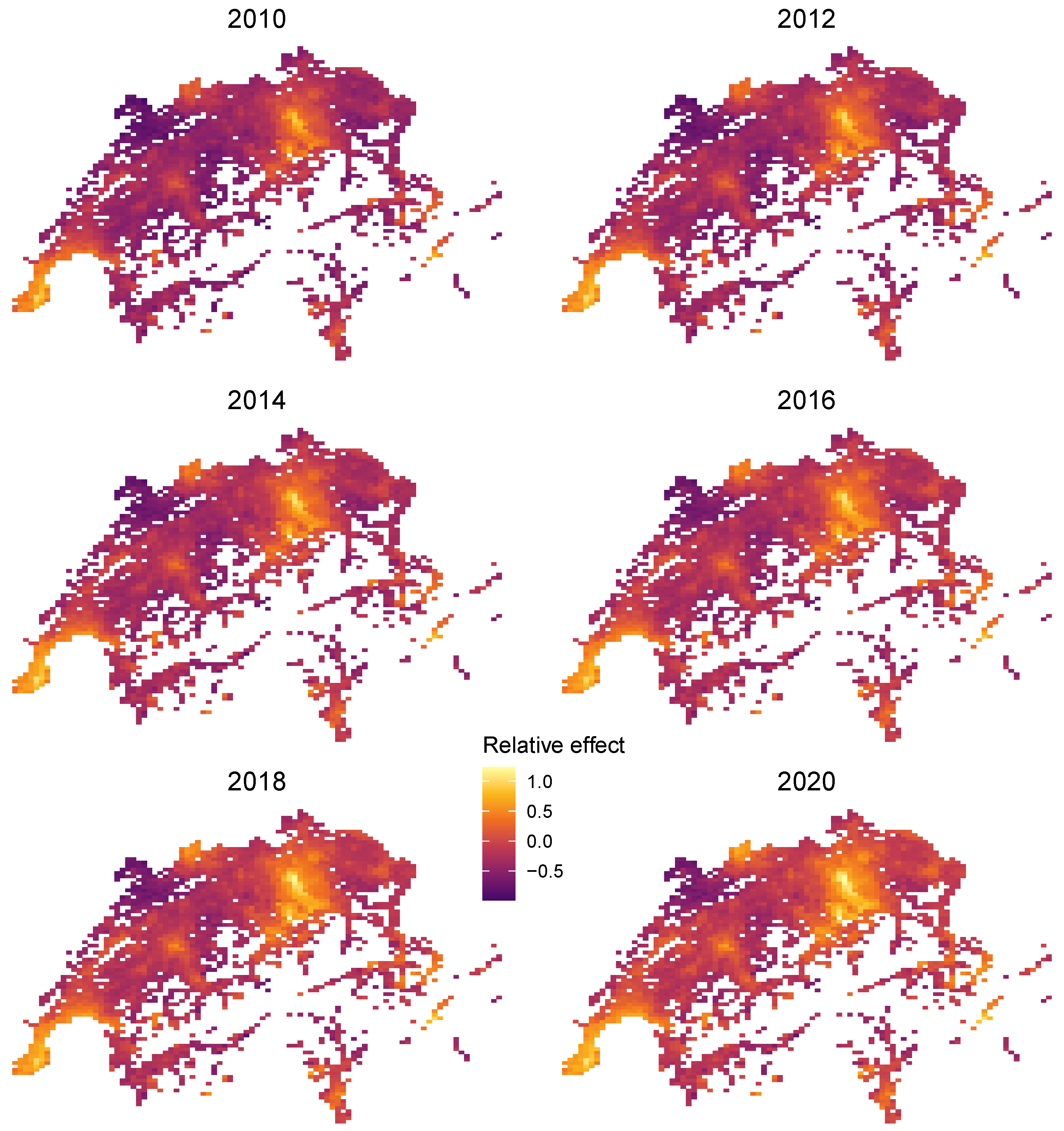
4.3.3. Extracting Time-Dependent Location Effects
5. Discussion and Conclusions
Author Contributions
Funding
Data Availability Statement
Acknowledgments
Conflicts of Interest
References
- Abadi, Martin, Paul Barham, Jianmin Chen, Zhifeng Chen, Andy Davis, Jeffrey Dean, Matthieu Devin, Sanjay Ghemawat, Geoffrey Irving, Michael Isard, and et al. 2016. Tensorflow: A system for large-scale machine learning. Paper presented at 12th USENIX Symposium on Operating Systems Design and Implementation (OSDI 16), Savannah, GA, USA, November 2–4; pp. 265–83. [Google Scholar] [CrossRef]
- Agarwal, Rishabh, Levi Melnick, Nicholas Frosst, Xuezhou Zhang, Ben Lengerich, Rich Caruana, and Geoffrey E. Hinton. 2021. Neural additive models: Interpretable machine learning with neural nets. Advances in Neural Information Processing Systems 34. [Google Scholar]
- Allaire, Joseph J., and François Chollet. 2021. Keras: R Interface to ’Keras’, R Package Version 2.4.0; Available online: https://CRAN.R-project.org/package=keras (accessed on 1 June 2021).
- Arik, Sercan Ömer, and Tomas Pfister. 2019. Tabnet: Attentive interpretable tabular learning. arXiv arXiv:2004.13912. [Google Scholar]
- Bühlmann, Peter, and Torsten Hothorn. 2007. Boosting Algorithms: Regularization, Prediction and Model Fitting. Statistical Science 22: 477–505. [Google Scholar] [CrossRef]
- Biecek, Przemyslaw, and Tomasz Burzykowski. 2021. Explanatory Model Analysis. New York: Chapman and Hall/CRC. [Google Scholar] [CrossRef]
- Chen, Tianqi, and Carlos Guestrin. 2016. Xgboost: A scalable tree boosting system. Paper presented at 22nd ACM SIGKDD International Conference on Knowledge Discovery and Data Mining,KDD ’16, San Francisco, CA, USA, August 13–17; New York: Association for Computing Machinery, pp. 785–94. [Google Scholar] [CrossRef] [Green Version]
- Chen, Tianqi, Tong He, Michael Benesty, Vadim Khotilovich, Yuan Tang, Hyunsu Cho, Kailong Chen, Rory Mitchell, Ignacio Cano, Tianyi Zhou, and et al. 2021. Xgboost: Extreme Gradient Boosting, R Package Version 1.4.1.1; Available online: https://CRAN.R-project.org/package=xgboost (accessed on 1 June 2021).
- Din, Allan, Martin Hoesli, and André Bender. 2001. Environmental variables and real estate prices. Urban Studies 38: 1989–2000. [Google Scholar] [CrossRef]
- Fahrmeir, Ludwig, Thomas Kneib, Stefan Lang, and Brian Marx. 2013. Regression: Models, Methods and Applications. Berlin: Springer. [Google Scholar] [CrossRef]
- Friedman, Jerome H. 2001. Greedy function approximation: A gradient boosting machine. The Annals of Statistics 29: 1189–232. [Google Scholar] [CrossRef]
- Friedman, Jerome H., and Bogdan E. Popescu. 2008. Predictive learning via rule ensembles. The Annals of Applied Statistics 2: 916–54. [Google Scholar] [CrossRef]
- Goldstein, Alex, Adam Kapelner, Justin Bleich, and Emil Pitkin. 2015. Peeking inside the black box: Visualizing statistical learning with plots of individual conditional expectation. Journal of Computational and Graphical Statistics 24: 44–65. [Google Scholar] [CrossRef]
- Hastie, Trevor, and Robert Tibshirani. 1986. Generalized Additive Models. Statistical Science 1: 297–310. [Google Scholar] [CrossRef]
- Hastie, Trevor, and Robert Tibshirani. 1990. Generalized Additive Models. Hoboken: Wiley Online Library. [Google Scholar]
- Hothorn, Torsten, Peter Bühlmann, Thomas Kneib, Matthias Schmid, and Benjamin Hofner. 2021. Mboost: Model-Based Boosting, R Package Version 2.9-5; Available online: https://CRAN.R-project.org/package=mboost (accessed on 5 July 2021).
- Hothorn, Torsten, Peter Bühlmann, Thomas Kneib, Matthias Schmid, and Benjamin Hofner. 2010. Model-based boosting 2.0. The Journal of Machine Learning Research 11: 2109–13. [Google Scholar]
- Kagie, Martijn, and Michiel Van Wezel. 2007. Hedonic price models and indices based on boosting applied to the dutch housing market. Intelligent Systems in Accounting, Finance & Management: International Journal 15: 85–106. [Google Scholar] [CrossRef]
- Ke, Guolin, Damien Soukhavong, James Lamb, Qi Meng, Thomas Finley, Taifeng Wang, Wei Chen, Weidong Ma, Qiwei Ye, Tie-Yan Liu, and et al. 2021. Lightgbm: Light Gradient Boosting Machine, R Package Version 3.2.1.99; Available online: https://github.com/microsoft/LightGBM (accessed on 13 August 2021).
- Ke, Guolin, Qi Meng, Thomas Finley, Taifeng Wang, Wei Chen, Weidong Ma, Qiwei Ye, and Tie-Yan Liu. 2017. Lightgbm: A highly efficient gradient boosting decision tree. In Advances in Neural Information Processing Systems. New York: Curran Associates, Inc., Volume 30, pp. 3149–57. [Google Scholar]
- Koenker, Roger. 2005. Quantile Regression. Econometric Society Monographs. Cambridge: Cambridge University Press. [Google Scholar] [CrossRef]
- Koenker, Roger. 2021. Quantreg: Quantile Regression, R Package Version 5.86; Available online: https://CRAN.R-project.org/package=quantreg (accessed on 13 August 2021).
- LeCun, Yann, Léon Bottou, Genevieve B. Orr, and Klaus-Robert Müller. 2012. Efficient backprop. In Neural Networks: Tricks of the Trade, 2nd ed. Edited by G. Montavon, G. B. Orr and K.-R. Müller. Volume 7700 of Lecture Notes in Computer Science. New York: Springer, pp. 9–48. [Google Scholar] [CrossRef]
- Lee, Simon C. K., Sheldon Lin, and Katrien Antonio. 2015. Delta Boosting Machine and Its Application in Actuarial Modeling. Sydney: Institute of Actuaries of Australia. [Google Scholar]
- Lou, Yin, Rich Caruana, and Johannes Gehrke. 2012. Intelligible models for classification and regression. Paper presented at 18th ACM SIGKDD International Conference on Knowledge Discovery and Data Mining, KDD ’12, Beijing, China, August 12–16; New York: Association for Computing Machinery, pp. 150–58. [Google Scholar] [CrossRef] [Green Version]
- Malpezzi, Stephen. 2003. Hedonic Pricing Models: A Selective and Applied Review. Hoboken: John Wiley & Sons, Ltd., Chapter 5. pp. 67–89. [Google Scholar] [CrossRef]
- Mayer, Michael. 2020. Github Issue. Available online: https://github.com/microsoft/LightGBM/issues/2884 (accessed on 6 March 2009).
- Mayer, Michael. 2021. Flashlight: Shed Light on Black Box Machine Learning Models, R Package Version 0.8.0; Available online: https://CRAN.R-project.org/package=flashlight (accessed on 1 June 2021).
- Mayer, Michael, Steven C. Bourassa, Martin Hoesli, and Donato Scognamiglio. 2019. Estimation and updating methods for hedonic valuation. Journal of European Real Estate Research 12: 134–50. [Google Scholar] [CrossRef] [Green Version]
- Molnar, Christoph. 2019. Interpretable Machine Learning. Available online: https://christophm.github.io/interpretable-ml-book (accessed on 1 July 2021).
- Nelder, John Ashworth, and Robert W. M. Wedderburn. 1972. Generalized linear models. Journal of the Royal Statistical Society: Series A (General) 135: 370–84. [Google Scholar] [CrossRef]
- Nori, Harsha, Samuel Jenkins, Paul Koch, and Rich Caruana. 2019. Interpretml: A unified framework for machine learning interpretability. arXiv arXiv:1909.00922. [Google Scholar]
- Prokhorenkova, Liudmila, Gleb Gusev, Aleksandr Vorobev, Anna Veronika Dorogush, and Andrey Gulin. 2018. Catboost: Unbiased boosting with categorical features. Paper presented at the 32nd International Conference on Neural Information Processing Systems, NIPS’18, Montréal, QC, Canada, December 3–8; New York: Curran Associates Inc., pp. 6639–49. [Google Scholar]
- Rügamer, David, Chris Kolb, and Nadja Klein. 2021. Semi-structured deep distributional regression: Combining structured additive models and deep learning. arXiv arXiv:2002.05777. [Google Scholar]
- Sangani, Darshan, Kelby Erickson, and Mohammad al Hasan. 2017. Predicting zillow estimation error using linear regression and gradient boosting. Paper presented at the 2017 IEEE 14th International Conference on Mobile Ad Hoc and Sensor Systems (MASS), Orlando, FL, USA, October 22–25; pp. 530–34. [Google Scholar] [CrossRef]
- Umlauf, Nikolaus, Daniel Adler, Thomas Kneib, Stefan Lang, and Achim Zeileis. 2012. Structured Additive Regression Models: An R Interface to BayesX. Working Papers 2012–10. Innsbruck: Faculty of Economics and Statistics, University of Innsbruck. [Google Scholar]
- Wei, Cankun, Meichen Fu, Li Wang, Hanbing Yang, Feng Tang, and Yuqing Xiong. 2022. The research development of hedonic price model-based real estate appraisal in the era of big data. Land 11: 334. [Google Scholar] [CrossRef]
- Wood, Simon N. 2017. Generalized Additive Models: An Introduction with R, 2nd ed. Boca Raton: CRC Press. [Google Scholar] [CrossRef]
- Worzala, Elaine, Margarita Lenk, and Ana Silva. 1995. An exploration of neural networks and its application to real estate valuation. Journal of Real Estate Research 10: 185–201. [Google Scholar] [CrossRef]
- Wüthrich, Mario V. 2020. Bias regularization in neural network models for general insurance pricing. European Actuarial Journal 10: 179–202. [Google Scholar] [CrossRef]
- Yoo, Sanglim, Jungho Im, and John E. Wagner. 2012. Variable selection for hedonic model using machine learning approaches: A case study in Onondaga County, NY. Landscape and Urban Planning 107: 293–306. [Google Scholar] [CrossRef]
- Zurada, Jozef, Alan S. Levitan, and Jian Guan. 2011. A comparison of regression and artificial intelligence methods in a mass appraisal context. Journal of Real Estate Research 33: 349–88. [Google Scholar] [CrossRef]


| XGBoost | LightGBM | |
|---|---|---|
| R | list(0, c(1, 2, 3)) | list(’A’, c(’B’, ’C’, ’D’)) |
| Python | ’[[0], [1, 2, 3]]’ | [[0], [1, 2, 3]] |
| Loss | XGBoost | LightGBM | |
|---|---|---|---|
| Squared error | "reg:squarederror" | "mse" | |
| Log loss | "binary:logistic" | "binary" | |
| Absolute error | median | - | "mae" |
| Quantile loss | p-quantile | - | "quantile" |
| Poisson loss | "count:poisson" | "poisson" | |
| Gamma loss | "reg:gamma" | "gamma" | |
| Tweedie loss | "reg:tweedie" | "tweedie" | |
| Huber-like loss | M-estimator | "reg:huber" | "huber" |
| Cox neg. log-lik | "survival:cox" | - |
| Variable Name | Symbol | Meaning |
|---|---|---|
| log_price | Y | Logarithmic sale price in USD |
| month_sold | T | Sale month in 2016 (1: January, ⋯, 12: December) |
| log_living | Living area in logarithmic square feet | |
| log_land | Land area in logarithmic square feet | |
| log_special | Logarithmic value of special features (e.g., swimming pool) | |
| age | Age of the structure when sold | |
| structure_quality | Measure of building quality (1: worst, 5: best) | |
| s_dist_highway | Square root of distance to nearest highway in 1000 ft | |
| s_dist_rail | Square root of distance to nearest rail line in 1000 ft | |
| dist_ocean | Distance to ocean in 1000 ft | |
| log_dist_water | Logarithmic distance in 1000 ft to nearest body of water | |
| s_dist_center | Square root of distance to central business district in 1000 ft | |
| s_dist_sub | Square root of distance to nearest subcenter in 1000 ft | |
| latitude | Latitude | |
| longitude | Longitude |
| Model | RMSE | R-Squared |
|---|---|---|
| OLS | 0.252 | 0.799 |
| XGB (unconstrained) | 0.132 | 0.945 |
| XGB STAR | 0.134 | 0.943 |
| OLS with XGB loc | 0.145 | 0.933 |
| NN STAR | 0.182 | 0.895 |
| mboost STAR | 0.159 | 0.920 |
| Model | MAE | RMSE |
|---|---|---|
| LGB (unconstrained) | 0.165 | 0.255 |
| LGB STAR | 0.168 | 0.259 |
| QR with LGB loc | 0.174 | 0.266 |
Publisher’s Note: MDPI stays neutral with regard to jurisdictional claims in published maps and institutional affiliations. |
© 2022 by the authors. Licensee MDPI, Basel, Switzerland. This article is an open access article distributed under the terms and conditions of the Creative Commons Attribution (CC BY) license (https://creativecommons.org/licenses/by/4.0/).
Share and Cite
Mayer, M.; Bourassa, S.C.; Hoesli, M.; Scognamiglio, D. Machine Learning Applications to Land and Structure Valuation. J. Risk Financial Manag. 2022, 15, 193. https://doi.org/10.3390/jrfm15050193
Mayer M, Bourassa SC, Hoesli M, Scognamiglio D. Machine Learning Applications to Land and Structure Valuation. Journal of Risk and Financial Management. 2022; 15(5):193. https://doi.org/10.3390/jrfm15050193
Chicago/Turabian StyleMayer, Michael, Steven C. Bourassa, Martin Hoesli, and Donato Scognamiglio. 2022. "Machine Learning Applications to Land and Structure Valuation" Journal of Risk and Financial Management 15, no. 5: 193. https://doi.org/10.3390/jrfm15050193
APA StyleMayer, M., Bourassa, S. C., Hoesli, M., & Scognamiglio, D. (2022). Machine Learning Applications to Land and Structure Valuation. Journal of Risk and Financial Management, 15(5), 193. https://doi.org/10.3390/jrfm15050193