On a Modified Weighted Exponential Distribution with Applications


Abstract
1. Introduction
1.1. State of Art
1.2. Contributions
- (i)
- The cdf can be written as where and , meaning that the MWE distribution also belongs to the family of generalized mixture of two exponential distributions, following the spirit of the distribution proposed by [16],
- (ii)
- The cdf is quite simple to manage and consequently, the MWE distribution can be studied in an-depth manner on all the theoretical and practical aspects,
- (iii)
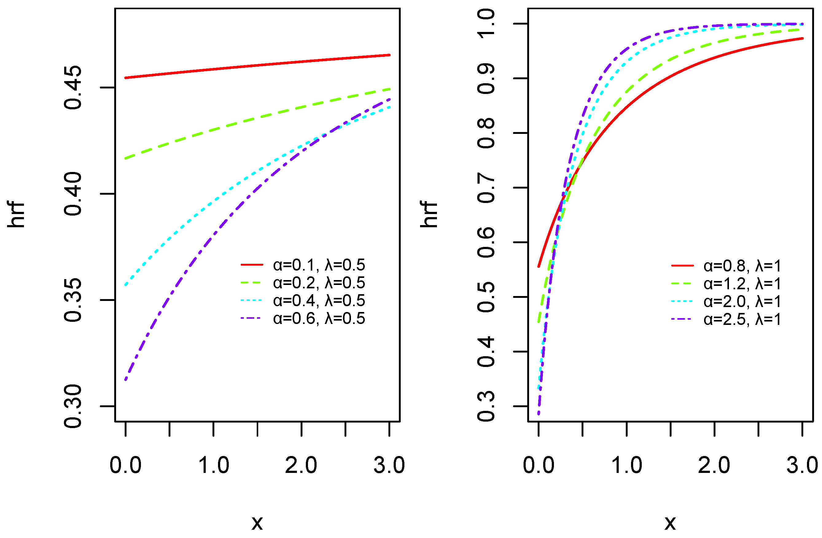
- Thanks to the parameter , the related pdf can be decreasing or unimodal, and the related hrf can be constant or increasing as proven later,
- (iv)
- In some concrete scenarios, the MWE model can be more efficient in data fitting than the exponential or WE models, among other lifetime models.
1.3. Paper Organization
2. Statistical Properties
2.1. Quantile and Survival Functions
2.2. Shapes of the Probability Density and Hazard Rate Functions
- if , then is decreasing.
- if , is unimodal, with the mode:
- if , thenwhich implies that is decreasing; the maximal point is obtained at .
- In the case, , we have , and one value of x vanished ; it is given by . For , we have and for , , implying that is a maximal point; it corresponds to the mode of the MWE distribution.
2.3. Moments and Moment Generating Function
2.4. Bonferroni and Lorenz Curves
2.5. Rényi Entropy
2.6. Reliability Characteristics of the MWE Distribution
2.7. Mean Residual Life Function
3. Parameters Estimation
3.1. Maximum Likelihood Estimates
3.2. Method of Moments Estimates
3.3. Least Squares and Weighted Least Squares Estimates
3.4. Cramér-von Mises Estimates
4. Simulation
5. Real Data Analysis
6. Concluding Remarks
Supplementary Materials
Author Contributions
Funding
Conflicts of Interest
References
- Gupta, R.D.; Kundu, D. A new class of weighted exponential distributions. Stat. A J. Theor. Appl. Stat. 2009, 43, 621–634. [Google Scholar] [CrossRef]
- Azzalini, A. A class of distributions which includes the normal ones. Scand. J. Stat. 1985, 12, 171–178. [Google Scholar]
- Das, S.; Kundu, D. On weighted exponential distribution and its length biased version. J. Indian Soc. Probab. Stat. 2016, 17, 57–77. [Google Scholar] [CrossRef]
- Roy, S.; Adnan, M.A.S. Wrapped weighted exponential distributions. Stat. Probab. Lett. 2012, 82, 77–83. [Google Scholar] [CrossRef]
- Hussian, M.A. A weighted inverted exponential distribution. Int. J. Adv. Stat. Probab. 2013, 1, 142–150. [Google Scholar] [CrossRef][Green Version]
- Dey, S.; Ali, S.; Park, C. Weighted exponential distribution: Properties and different methods of estimation. J. Stat. Comput. Simul. 2015, 85, 3641–3661. [Google Scholar] [CrossRef]
- Oguntunde, P.E. On the exponentiated weighted exponential distribution and its basic statistical properties. Appl. Sci. Rep. 2015, 10, 160–167. [Google Scholar]
- Kharazmi, O.; Mahdavi, A.; Fathizadeh, M. Generalized weighted exponential distribution. Commun. Stat. Simul. Comput. 2015, 44, 1557–1569. [Google Scholar] [CrossRef]
- Alqallaf, F.; Ghitany, M.E.; Agostinelli, C. Weighted exponential distribution: Different methods of estimations. Appl. Math. Inf. Sci. 2015, 9, 1167–1173. [Google Scholar]
- Perveen, Z.; Ahmed, Z.; Ahmad, M. On size-biased double weighted exponential distribution (SDWED). Open J. Stat. 2016, 6, 917–930. [Google Scholar] [CrossRef][Green Version]
- Mahdavi, A.; Jabbari, L. An extended weighted exponential distribution. J. Mod. Appl. Stat. Methods 2017, 16, 296–307. [Google Scholar] [CrossRef]
- Oguntunde, P.E.; Ilori, K.A.; Okagbue, H.I. The inverted weighted exponential distribution with applications. Int. J. Adv. Appl. Sci. 2018, 5, 46–50. [Google Scholar] [CrossRef]
- Mallick, A.; Ghosh, I.; Dey, S.; Kumar, D. Bounded weighted exponential distribution with applications. Am. J. Math. Manag. Sci. 2022, 40, 68–87. [Google Scholar] [CrossRef]
- Bakouch, H.S.; Hussain, T.; Chesneau, C.; Khan, M.N. On a weighted exponential distribution with a logarithmic weight: Theory and applications. Afr. Mat. 2021, 32, 789–810. [Google Scholar] [CrossRef]
- Tomy, L.; Jose, M.; Veena, G. A review on recent generalizations of exponential distribution. Biom. Biostat. Int. J. 2020, 9, 152–156. [Google Scholar] [CrossRef]
- Yang, Y.; Tian, W.; Tong, T. Generalized Mixtures of Exponential Distribution and Associated Inference. Mathematics 2021, 9, 1371. [Google Scholar] [CrossRef]
- Giorgi, G.M.; Nadrajah, S. Bonferroni and Gini indices for various parametric families of distributions. Metron 2010, 68, 23–46. [Google Scholar] [CrossRef]
- Amigó, J.M.; Balogh, S.G.; Hernéz, S. A Brief Review of Generalized Entropies. Entropy 2018, 20, 813. [Google Scholar] [CrossRef]
- Swain, J.J.; Venkatraman, S.; Wilson, J.R. Least-squares estimation of distribution functions in Johnson’s translation system. J. Stat. Comput. Simul. 1988, 29, 271–297. [Google Scholar] [CrossRef]
- Arshad, M.; Khetan, M.; Kumar, V.; Pathak, A.K. Record-Based Transmuted Generalized Linear Exponential Distribution with Increasing, Decreasing and Bathtub Shaped Failure Rates. arXiv 2021, arXiv:2107.09316. [Google Scholar]
- Broyden, C.G. The convergence of a class of double-rank minimization algorithms 1. general considerations. IMA J. Appl. Math. 1970, 6, 76–90. [Google Scholar] [CrossRef]
- Fletcher, R. A new approach to variable metric algorithms. Comput. J. 1970, 13, 317–322. [Google Scholar] [CrossRef]
- Goldfarb, D. A family of variable-metric methods derived by variational means. Math. Comput. 1970, 24, 23–26. [Google Scholar] [CrossRef]
- Shanno, D.F. Conditioning of quasi-Newton methods for function minimization. Math. Comput. 1970, 24, 647–656. [Google Scholar] [CrossRef]
- Kenneth, P.B.; Anderson, D.R. Model Selection and Multi-Model Inference: A Practical Information-Theoretic Approach, 2nd ed.; Springer: Berlin/Heidelberg, Germany, 2002. [Google Scholar]
- Gupta, R.D.; Kundu, D. Theory & methods: Generalized exponential distributions. Aust. N. Z. J. Stat. 1999, 41, 173–188. [Google Scholar]
- Lai, C.D.; Murthy, D.; Xie, M. Weibull Distributions and Their Applications. In Springer Handbook of Engineering Statistics; Pham, H., Ed.; Springer: London, UK, 2006. [Google Scholar]
- Aldeni, M.; Lee, C.; Famoye, F. Families of distributions arising from the quantile of generalized lambda distribution. J. Stat. Distrib. Appl. 2017, 4, 25. [Google Scholar] [CrossRef]


| V | |||||
|---|---|---|---|---|---|
| 0.5000 | 0.2000 | 2.2778 | 4.8488 | 1.8639 | 8.1028 |
| 0.5000 | 0.4000 | 2.4082 | 4.9996 | 1.7628 | 7.5801 |
| 0.5000 | 0.6000 | 2.4688 | 4.9521 | 1.7198 | 7.4207 |
| 0.5000 | 0.8000 | 2.4938 | 4.8535 | 1.7089 | 7.4265 |
| 0.5000 | 1.0000 | 2.5000 | 4.7500 | 1.7146 | 7.5042 |
| 0.5000 | 1.2000 | 2.4959 | 4.6557 | 1.7283 | 7.6100 |
| 0.5000 | 1.4000 | 2.4861 | 4.5739 | 1.7454 | 7.7230 |
| 1.2000 | 0.4000 | 3.1198 | 7.2745 | 1.7283 | 7.6100 |
| 1.2000 | 0.6000 | 2.0799 | 3.2331 | 1.7283 | 7.6100 |
| 1.2000 | 0.8000 | 1.5599 | 1.8186 | 1.7283 | 7.6100 |
| 1.2000 | 1.0000 | 1.2479 | 1.1639 | 1.7283 | 7.6100 |
| 1.2000 | 1.2000 | 1.0399 | 0.8083 | 1.7283 | 7.6100 |
| 1.2000 | 1.4000 | 0.8914 | 0.5938 | 1.7283 | 7.6100 |
| 1.2000 | 1.6000 | 0.7800 | 0.4547 | 1.7283 | 7.6100 |
| n | Estimate | Bias | MSE | ||
|---|---|---|---|---|---|
| 50 | MLE | 0.6411 | −0.0459 | 6.4825 | 0.0195 |
| MOME | 0.7038 | −0.0356 | 0.9878 | 0.0217 | |
| OLSE | 0.3002 | −0.0956 | 1.0082 | 0.0272 | |
| WLSE | 0.3090 | −0.0840 | 1.2376 | 0.0246 | |
| CME | 0.4610 | −0.0800 | 1.3098 | 0.0244 | |
| 100 | MLE | 0.2742 | −0.0446 | 0.7519 | 0.0109 |
| MOME | 0.6530 | −0.0367 | 0.8751 | 0.0124 | |
| OLSE | 0.1904 | −0.0828 | 0.4913 | 0.0172 | |
| WLSE | 0.1782 | −0.0712 | 0.5446 | 0.0147 | |
| CME | 0.2772 | −0.0727 | 0.6083 | 0.0152 | |
| 200 | MLE | 0.1165 | −0.0409 | 0.1834 | 0.0059 |
| MOME | 0.5855 | −0.0330 | 0.7346 | 0.0058 | |
| OLSE | 0.1391 | −0.0674 | 0.2210 | 0.0099 | |
| WLSE | 0.1177 | −0.0573 | 0.1701 | 0.0080 | |
| CME | 0.1794 | −0.0619 | 0.2406 | 0.0090 | |
| 500 | MLE | 0.0620 | −0.0365 | 0.0317 | 0.0028 |
| MOME | 0.5134 | −0.0274 | 0.5407 | 0.0023 | |
| OLSE | 0.0981 | −0.0527 | 0.0693 | 0.0047 | |
| WLSE | 0.0822 | −0.0457 | 0.0532 | 0.0037 | |
| CME | 0.1136 | −0.0506 | 0.0744 | 0.0044 |
| n | Estimate | Bias | MSE | ||
|---|---|---|---|---|---|
| 50 | MLE | 0.7146 | −0.0072 | 4.7462 | 0.0201 |
| MOME | 0.1304 | −0.0103 | 0.5513 | 0.0270 | |
| OLSE | 0.1174 | −0.0410 | 1.9271 | 0.0243 | |
| WLSE | 0.2331 | −0.0352 | 2.9491 | 0.0223 | |
| CME | 0.3445 | −0.0250 | 2.2686 | 0.0227 | |
| 100 | MLE | 0.4174 | −0.0078 | 3.5071 | 0.0116 |
| MOME | −0.0152 | −0.0182 | 0.5008 | 0.0158 | |
| OLSE | 0.0858 | −0.0207 | 1.5188 | 0.0137 | |
| WLSE | 0.1388 | −0.0166 | 2.0104 | 0.0126 | |
| CME | 0.2204 | −0.0114 | 1.6787 | 0.0130 | |
| 200 | MLE | 0.0649 | −0.0017 | 1.5542 | 0.0062 |
| MOME | −0.1548 | −0.0145 | 0.4094 | 0.0086 | |
| OLSE | −0.0483 | −0.0052 | 0.9840 | 0.0072 | |
| WLSE | −0.0602 | −0.0028 | 1.0602 | 0.0064 | |
| CME | 0.0158 | −0.0002 | 0.9988 | 0.0069 | |
| 500 | MLE | −0.2141 | 0.0089 | 0.3936 | 0.0022 |
| MOME | −0.3341 | −0.0051 | 0.3066 | 0.0030 | |
| OLSE | −0.2070 | 0.0160 | 0.2761 | 0.0026 | |
| WLSE | −0.2370 | 0.0141 | 0.2548 | 0.0023 | |
| CME | −0.1802 | 0.0179 | 0.2866 | 0.0026 |
| n | Estimate | Bias | MSE | ||
|---|---|---|---|---|---|
| 50 | MLE | 0.2723 | 0.0012 | 4.7454 | 0.0162 |
| MOME | −0.0325 | 0.0342 | 0.3603 | 0.0200 | |
| OLSE | 0.0888 | −0.0405 | 2.2201 | 0.0202 | |
| WLSE | 0.2376 | −0.0312 | 2.8245 | 0.0182 | |
| CME | 0.2884 | −0.0303 | 2.2121 | 0.0192 | |
| 100 | MLE | −0.0163 | 0.0078 | 2.0841 | 0.0083 |
| MOME | −0.0247 | 0.0291 | 0.3181 | 0.0096 | |
| OLSE | 0.1303 | −0.0244 | 1.7747 | 0.0103 | |
| WLSE | 0.2232 | −0.0166 | 2.0862 | 0.0091 | |
| CME | 0.2683 | −0.0205 | 1.8484 | 0.0099 | |
| 200 | MLE | −0.2227 | 0.0148 | 0.6364 | 0.0042 |
| MOME | 0.0318 | 0.0267 | 0.2444 | 0.0046 | |
| OLSE | 0.1333 | −0.0099 | 1.3872 | 0.0050 | |
| WLSE | 0.1396 | −0.0039 | 1.3626 | 0.0044 | |
| CME | 0.2233 | −0.0092 | 1.4512 | 0.0049 | |
| 500 | MLE | −0.3446 | 0.0196 | 0.2372 | 0.0017 |
| MOME | 0.1420 | 0.0222 | 0.1582 | 0.0018 | |
| OLSE | 0.0786 | 0.0008 | 0.8774 | 0.0021 | |
| WLSE | −0.0197 | 0.0063 | 0.4987 | 0.0018 | |
| CME | 0.1225 | 0.0006 | 0.9003 | 0.0021 |
| Model | MLEs (Standard Errors) |
|---|---|
| MWE | , |
| W | , |
| G | , |
| GE | , |
| WE | , |
| MOME | OLSE | WLSE | CME | |
|---|---|---|---|---|
| 1.8324 | 0.2399 | 0.3517 | 0.3289 | |
| 0.0417 | 0.0344 | 0.0373 | 0.0358 |
| Model | AIC | KS | p(KS) | CVM | p(CVM) | AD | p(AD) |
|---|---|---|---|---|---|---|---|
| MWE | 443.8088 | 0.0955 | 0.7161 | 0.1015 | 0.5796 | 0.8336 | 0.4568 |
| W | 444.6980 | 0.1113 | 0.5290 | 0.1269 | 0.4698 | 0.8907 | 0.4195 |
| G | 444.5201 | 0.1226 | 0.4074 | 0.1477 | 0.3976 | 0.8702 | 0.4325 |
| GE | 444.4178 | 0.1243 | 0.3903 | 0.1520 | 0.3844 | 0.8719 | 0.4314 |
| WE | 468.9382 | 0.1544 | 0.1658 | 0.2851 | 0.1489 | 4.6374 | 0.0043 |
| Distribution | MLEs (Standard Errors) |
|---|---|
| MWE | , |
| W | , |
| G | , |
| GE | , |
| WE | , |
| MOME | OLSE | WLSE | CME | |
|---|---|---|---|---|
| 0.0003 | 5.5633 | 6.4080 | 5.0124 | |
| 0.1003 | 0.1294 | 0.1263 | 0.1312 |
| Model | AIC | KS | p(KS) | CVM | p(CVM) | AD | p(AD) | |
|---|---|---|---|---|---|---|---|---|
| MWE | 827.2080 | 831.2080 | 0.0619 | 0.7100 | 0.0842 | 0.6689 | 0.5012 | 0.7453 |
| W | 830.1968 | 834.1968 | 0.0663 | 0.6272 | 0.1380 | 0.4286 | 0.8743 | 0.4302 |
| G | 828.7471 | 832.7471 | 0.0692 | 0.5722 | 0.1178 | 0.5049 | 0.6849 | 0.5713 |
| GE | 828.1806 | 832.1806 | 0.0684 | 0.5877 | 0.1100 | 0.5389 | 0.6275 | 0.6221 |
| WE | 828.3536 | 832.3536 | 0.0594 | 0.7579 | 0.0757 | 0.7182 | 0.4816 | 0.7653 |
Publisher’s Note: MDPI stays neutral with regard to jurisdictional claims in published maps and institutional affiliations. |
© 2022 by the authors. Licensee MDPI, Basel, Switzerland. This article is an open access article distributed under the terms and conditions of the Creative Commons Attribution (CC BY) license (https://creativecommons.org/licenses/by/4.0/).
Share and Cite
Chesneau, C.; Kumar, V.; Khetan, M.; Arshad, M. On a Modified Weighted Exponential Distribution with Applications. Math. Comput. Appl. 2022, 27, 17. https://doi.org/10.3390/mca27010017
Chesneau C, Kumar V, Khetan M, Arshad M. On a Modified Weighted Exponential Distribution with Applications. Mathematical and Computational Applications. 2022; 27(1):17. https://doi.org/10.3390/mca27010017
Chicago/Turabian StyleChesneau, Christophe, Vijay Kumar, Mukti Khetan, and Mohd Arshad. 2022. "On a Modified Weighted Exponential Distribution with Applications" Mathematical and Computational Applications 27, no. 1: 17. https://doi.org/10.3390/mca27010017
APA StyleChesneau, C., Kumar, V., Khetan, M., & Arshad, M. (2022). On a Modified Weighted Exponential Distribution with Applications. Mathematical and Computational Applications, 27(1), 17. https://doi.org/10.3390/mca27010017