
Conditional Inference in Small Sample Scenarios Using a Resampling Approach


Abstract
:1. Introduction
2. Theoretical Background
2.1. Psychometric Model
2.2. Statistical Tests
3. Resampling Algorithms and Computational Issues
4. Design
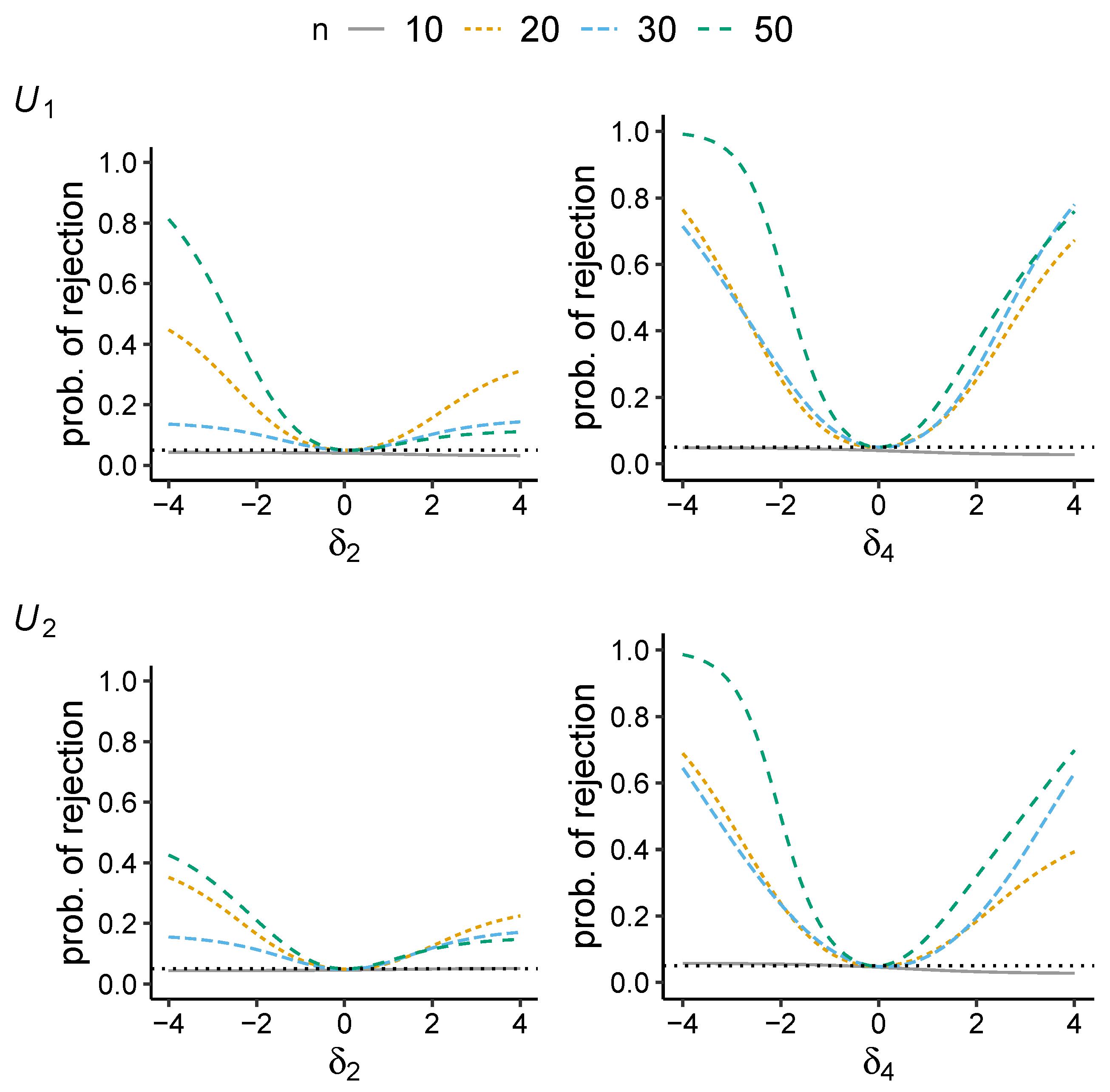
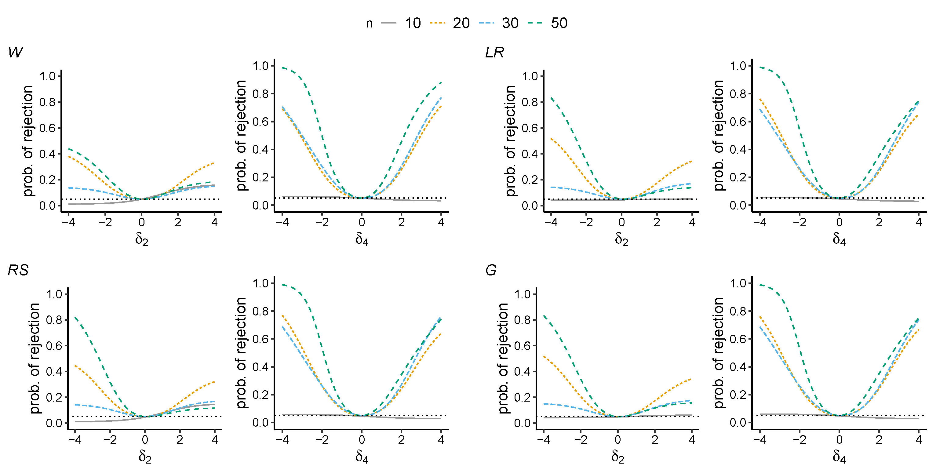
5. Results
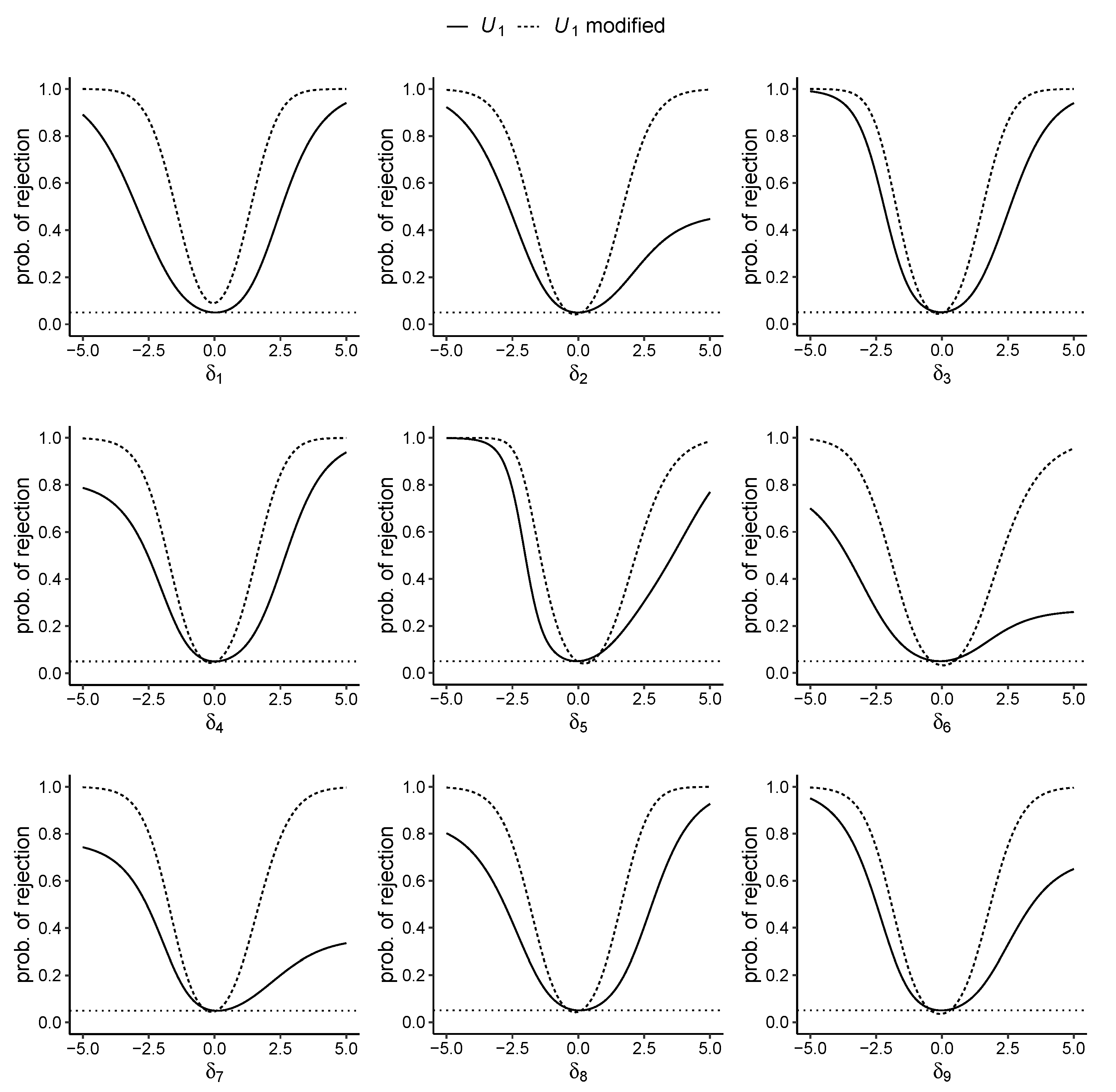
6. Examples of Modifications of the Tests
7. Final Remarks
Author Contributions
Funding
Institutional Review Board Statement
Informed Consent Statement
Data Availability Statement
Conflicts of Interest
References
- Rodgers, J.L. The Bootstrap, the Jackknife, and the Randomization Test: A Sampling Taxonomy. Multivar. Behav. Res. 1999, 34, 441–456. [Google Scholar] [CrossRef]
- Quenouille, M.H. Notes on bias in estimation. Biometrika 1956, 43, 353–360. [Google Scholar] [CrossRef]
- Tukey, J. Bias and confidence in not quite large samples. Ann. Math. Stat. 1958, 29, 614. [Google Scholar]
- Efron, B. The 1977 RIETZ lecture: Bootstrap Methods. Ann. Stat. 1979, 7, 1–26. [Google Scholar]
- Efron, B.; Tibshirani, R.J. An Introduction to the Bootstrap; Springer: New York, NY, USA, 1993. [Google Scholar]
- Romano, J.P.; Shaikh, A.M.; Wolf, M. Hypothesis Testing in Econometrics. Annu. Rev. Econ. 2010, 2, 75–104. [Google Scholar] [CrossRef] [Green Version]
- Davison, A.C.; Hinkley, D.V. Bootstrap Methods and Their Application; Cambridge University Press: Cambridge, UK, 1997. [Google Scholar]
- Chernick, M.R. Bootstrap Methods: A Guide for Practitioners and Researchers, 2nd ed.; Wiley: New York, NY, USA, 2008. [Google Scholar]
- Chernick, M.R.; LaBudde, R.A. An Introduction to Bootstrap Methods with Applications to R; Wiley: New York, NY, USA, 2011. [Google Scholar]
- Rasch, G. Probabilistic Models for Some Intelligence and Attainment Tests; Danish Institute for Educational Research: Kopenhagen, Demark, 1960. [Google Scholar]
- Fischer, G.H.; Molenaar, I.W. Rasch Models: Foundations, Recent Developments, and Applications; Springer: New York, NY, USA, 1995. [Google Scholar]
- Davier, M.V. Bootstrapping goodness-of-fit statistics for sparse categorical data: Results of a Monte Carlo study. Methods Psychol. Res. Online 1997, 2, 29–48. [Google Scholar]
- Heene, M.; Draxler, C.; Ziegler, M.; Bühner, M. Performance of the bootstrap Rasch model test under violations of non-intersecting item response functions. Psychol. Test Assess. Model. 2011, 53, 283–294. [Google Scholar]
- Alexandrowicz, R.W.; Draxler, C. Testing the Rasch model with the conditional likelihood ratio test: Sample size requirements and bootstrap algorithms. J. Stat. Distrib. Appl. 2016, 3, 1–25. [Google Scholar] [CrossRef] [Green Version]
- Ponocny, I. Nonparametric goodness-of-fit tests for the Rasch model. Psychometrika 2001, 66, 437–459. [Google Scholar] [CrossRef]
- Chen, Y.; Small, D. Exact Tests for the Rasch Model via Sequential Importance Sampling. Psychometrika 2005, 70, 11–30. [Google Scholar] [CrossRef]
- Verhelst, N.D. An efficient MCMC algorithm to sample binary matrices with fixed marginals. Psychometrika 2008, 73, 705–728. [Google Scholar] [CrossRef]
- Miller, J.W.; Harrison, M.T. Exact sampling and counting for fixed-margin matrices. Ann. Stat. 2013, 41, 1569–1592. [Google Scholar] [CrossRef] [Green Version]
- Draxler, C.; Zessin, J. The power function of conditional tests of the Rasch model. AStA Adv. Stat. Anal. 2015, 99, 367–378. [Google Scholar] [CrossRef]
- Draxler, C.; Nolte, J.P. Computational Precision of the Power Function for Conditional Tests of Assumptions of the Rasch Model. Open J. Stat. 2018, 8, 873. [Google Scholar] [CrossRef] [Green Version]
- Draxler, C.; Dahm, S. Conditional or Pseudo Exact Tests with an Application in the Context of Modeling Response Times. Psych 2020, 2, 17. [Google Scholar] [CrossRef]
- Verhelst, N.D.; Hatzinger, R.; Mair, P. The Rasch Sampler. J. Stat. Softw. 2007, 20, 1–14. [Google Scholar] [CrossRef]
- Lehmann, E.L.; Romano, J.P. Testing Statistical Hypotheses, 3rd ed.; Springer: New York, NY, USA, 2005. [Google Scholar]
- Draxler, C. A Note on a Discrete Probability Distribution Derived from the Rasch Model. Adv. Appl. Stat. Sci. 2011, 6, 665–673. [Google Scholar]
- Agresti, A. Categorical Data Analysis, 3rd ed.; Wiley: Hoboken, NJ, USA, 2013. [Google Scholar]
- Neyman, J.; Pearson, E.S. On the Use and Interpretation of certain test criteria for purposes of statistical inference. Biometrika 1928, 20, 263–294. [Google Scholar]
- Wilks, S.S. The large-sample distribution of the likelihood ratio for testing composite hypotheses. Ann. Math. Stat. 1938, 9, 60–62. [Google Scholar] [CrossRef]
- Wald, A. Tests of statistical hypotheses concerning several parameters when the number of observations is large. Trans. Am. Math. Soc. 1943, 54, 426–482. [Google Scholar] [CrossRef]
- Rao, C.R. Large sample tests of statistical hypotheses concerning several parameters with applications to problems of estimation. Math. Proc. Camb. Philos. 1948, 44, 50–57. [Google Scholar]
- Silvey, S.D. The lagrangian multiplier test. Ann. Math. Stat. 1959, 30, 389–407. [Google Scholar] [CrossRef]
- Terrell, G.R. The gradient statistic. Comput. Sci. Stat. 2002, 34, 206–215. [Google Scholar]
- Lemonte, A.J. The Gradient Test. Another Likelihood-Based Test; Academic Press: London, UK, 2016; ISBN 978-0-12-803596-2. [Google Scholar]
- Draxler, C.; Kurz, A.; Lemonte, A.J. The gradient test and its finite sample size properties in a conditional maximum likelihood and psychometric modeling context. Commun. Stat. Simul. Comput. 2020, 1–19. [Google Scholar] [CrossRef]
- Snijders, T.A.B. Enumeration and simulation methods for 0–1 matrices with given marginals. Psychometrika 1991, 56, 397–417. [Google Scholar] [CrossRef]
- Chen, Y.; Diaconis, P.; Holmes, S.P.; Liu, J.S. Sequential Monte Carlo Methods for Statistical Analysis of Tables. J. Am. Stat. Assoc. 1991, 100, 109–120. [Google Scholar] [CrossRef]
- Besag, J.; Clifford, P. Generalized Monte Carlo significance tests. Biometrika 1989, 76, 633–642. [Google Scholar] [CrossRef]
- Strona, G.; Nappo, D.; Boccacci, F.; Fattorini, S.; San-Miguel-Ayanz, J. A fast and unbiased procedure to randomize ecological binary matrices with fixed row and column totals. Nat. Commun. 2014, 5, 4114. [Google Scholar] [CrossRef]
- Carstens, C.J. Proof of uniform sampling of binary matrices with fixed row sums and column sums for the fast Curveball algorithm. Phys. Rev. E 2015, 91, 042812. [Google Scholar] [CrossRef]
- Rechner, S. Markov Chain Monte Carlo Algorithms for the Uniform Sampling of Combinatorial Objects. Ph.D. Thesis, Martin-Luther-Universität Halle-Wittenberg, Halle, Germany, 2018. [Google Scholar] [CrossRef]
- Mair, P.; Hatzinger, R. Extended Rasch modeling: The eRm package for the application of IRT models in R. J. Stat. Softw. 2007, 20, 1–20. [Google Scholar] [CrossRef] [Green Version]
- Draxler, C.; Kurz, A. Tcl: Testing in Conditional Likelihood Context, R Package Version 0.1.1; 2021. Available online: https://CRAN.R-project.org/package=tcl (accessed on 31 August 2021).
- Fischer, G.H. On the existence and uniqueness of maximum-likelihood estimates in the Rasch model. Psychometrika 1981, 46, 59–77. [Google Scholar] [CrossRef]
- Glas, C.A.W.; Verhelst, N.D. Testing the Rasch Model; Springer: New York, NY, USA, 1995; pp. 69–95. [Google Scholar]
- Draxler, C.; Alexandrowicz, R.W. Sample size determination within the scope of conditional maximum likelihood estimation with special focus on testing the Rasch model. Psychometrika 2015, 80, 897–919. [Google Scholar] [CrossRef]

Publisher’s Note: MDPI stays neutral with regard to jurisdictional claims in published maps and institutional affiliations. |
© 2021 by the authors. Licensee MDPI, Basel, Switzerland. This article is an open access article distributed under the terms and conditions of the Creative Commons Attribution (CC BY) license (https://creativecommons.org/licenses/by/4.0/).
Share and Cite
Draxler, C.; Kurz, A. Conditional Inference in Small Sample Scenarios Using a Resampling Approach. Stats 2021, 4, 837-849. https://doi.org/10.3390/stats4040049
Draxler C, Kurz A. Conditional Inference in Small Sample Scenarios Using a Resampling Approach. Stats. 2021; 4(4):837-849. https://doi.org/10.3390/stats4040049
Chicago/Turabian StyleDraxler, Clemens, and Andreas Kurz. 2021. "Conditional Inference in Small Sample Scenarios Using a Resampling Approach" Stats 4, no. 4: 837-849. https://doi.org/10.3390/stats4040049
APA StyleDraxler, C., & Kurz, A. (2021). Conditional Inference in Small Sample Scenarios Using a Resampling Approach. Stats, 4(4), 837-849. https://doi.org/10.3390/stats4040049