
Univariate and Multivariate GARCH Models Applied to Bitcoin Futures Option Pricing


1
Department of Actuarial Science, University of Pretoria, Private Bag X20, Hatfield 0028, South Africa
2
Department of Finance and Investment Management, University of Johannesburg, P.O. Box 524, Aucklandpark 2006, South Africa
3
Department of Mathematics and Applied Mathematics, University of Pretoria, Private Bag X20, Hatfield 0028, South Africa
*
Author to whom correspondence should be addressed.
†
These authors contributed equally to this work.
J. Risk Financial Manag. 2021, 14(6), 261; https://doi.org/10.3390/jrfm14060261
Submission received: 5 May 2021
/
Revised: 2 June 2021
/
Accepted: 7 June 2021
/
Published: 10 June 2021
(This article belongs to the Special Issue Recent Developments in Digital Currency: Time Series Analysis, Theory and Practice)
Abstract
:In this paper, the Heston–Nandi futures option pricing model is applied to Bitcoin futures options. The model prices are compared to market prices to give an indication of the pricing performance. In addition, a multivariate Bitcoin futures option pricing methodology based on a multivatiate GARCH model is developed. The empirical results show that a symmetric model is a better fit when applied to Bitcoin futures returns, and also produces more accurate option prices compared to market prices for two out of three expiry dates considered.
1. Introduction
Cryptocurrencies, and especially Bitcoin, have received a lot of attention in the financial modelling literature in recent years. Financial modelling researchers and practitioners are faced with the problem of price discovery when derivatives on a new asset class are introduced. The focus of this paper is price discovery in the Bitcoin futures option market. Abraham (2020) explains that a valuation model for Bitcoin futures options can provide insight into a central-bank free currency. We consider vanilla options (univariate) and spread options (multivariate).
Modelling the historical returns of an asset as a univariate generalised autoregressive conditional heterskedasticty (GARCH) process is often used as a basis for price discovery in illiquid derivative markets. The model by Heston and Nandi (2000) is often used because it has a convenient closed-form solution. However, this is usually applied to spot price dynamics. This model was extended to futures options on commodities by Li (2019a). The Chicago Mercantile Exchange (CME) was the first established exchange to launch Bitcoin futures options in the first quarter of 2020 (Bharadwaj 2021). Therefore, Bitcoin futures options are actively traded, and model prices can be compared to market prices to give an indication of pricing performance.
An important factor to consider is the ability to model joint dynamics for the pricing of multivariate derivatives, when pricing derivatives on a new asset class. According to Alexander and Heck (2020), crypto-asset futures are exposed to significant basis risk. Therefore, spread options on Bitcoin futures are ideal for hedging basis risk. Spread options on Bitcoin futures do not actively trade. In this study, we consider a modelling approach for price discovery in the Bitcoin futures spread option market. The approach is based on work by Rombouts and Stentoft (2011), who derived the risk-neutral dynamics of the spot price processes for a general class of multivariate heteroskedasticity models. In this study, the model by Rombouts and Stentoft (2011) is extended to multivariate futures options.
The rest of this paper is structured as follows: Section 2 reviews the recent and relevant literature, Section 3 focuses on the theoretical framework (both univariate and mulitvariate options on Bitcoin futures), Section 4 presents the empirical results, and finally, Section 5 provides concluding remarks.
2. Literature Review
Research focusing on GARCH models applied to Bitcoin (and other crypto-assets) and Bitcoin derivative pricing is well documented in the literature. In a recent study, Fassas et al. (2020) made use of a vector error correction model to investigate the price discovery process in the Bitcoin market. Their empirical results indicate that volume traded in the futures market is more important than the volume traded in the decentralised spot market when incorporating new information about the value Bitcoin. In addition, Fassas et al. (2020) consider the volatility transmission between the Bitcoin spot and futures market by using multivariate GARCH models (BEKK and dynamic-conditional-correlation). There is evidence of cross-market effects when the variability of Bitcoin spot and futures returns are considered.
It is important to consider a reasonable forecast of Bitcoin returns when trading Bitcoin derivatives. In a study focusing on the use of information on the US–China trade war to forecast Bitcoin returns, Plakandaras et al. (2021) made use of ordinary least squares regression, least absolute shrinkage and selection operator techniques, and support vector regression. The authors also controlled for explanatory variables, which include: financial indices (including the volatility index), exchange rates, commodity prices, political uncertainty indices, and Bitcoin characteristics. Their empirical results indicate that Bitcoin returns are not affected by trade-related uncertainties.
In a recent paper, Shahzad et al. (2019) made use of the bivariate cross-quantilogram to determine whether Bitcoin exhibits safe haven properties (during extreme market conditions) for equity investments. The authors extend the work by Baur and Lucey (2010) to incorporate weak and strong safe haven assets. Furthermore, the safe haven properties of Bitcoin were also compared to those of gold and the general commodity index. Shahzad et al. (2019) conclude that Bitcoin, gold, and the general commodity index can be considered (at best) a weak safe haven asset in some cases.
Fang et al. (2019) made use of the GARCH-MIDAS model to investigate how the long-run volatility of Bitcoin, global equities, bonds, and commodities evolves with global economic policy uncertainty. Their empirical results indicate that global economic policy uncertainty is significant for all variables, except bonds. Furthermore, Fang et al. (2019) also considered the impact of global economic policy uncertainty on the correlation between Bitcoin and global equities, commodities, and bonds. Based on the empirical results, the authors argue that Bitcoin can act as a hedge under specific economic uncertainty conditions.
In a study highlighting the role of Bitcoin futures, Chen and So (2020) focused on the relationship between Bitcoin spot and futures prices, with the focus on hedging. Chen and So (2020) tested the hedge performance of the naive method, ordinary least squares, and a dynamic hedge based on a bivariate BEKK-GJR-GARCH model. The results show that the hedge based on the bivariate GARCH model is the most reliable. Furthermore, Chen and So (2020) also show that the structure of Bitcoin volatility is significantly different after the introduction of Bitcoin futures.
In a recent study, Venter et al. (2020) applied symmetric and asymmetric GARCH option pricing models to Bitcoin and CRIX (Cryptocurrency Index). The model Bitcoin option prices were compared to market option prices, which shows that the GARCH option pricing model produces reasonable price discovery. Furthermore, the implied volatility surfaces generated using symmetric and asymmetric GARCH models were compared. This comparison indicates that there is not a significant difference, implying that the symmetric model is a better choice as it is more efficient.
Jalan et al. (2020) focused on the pricing and risk of Bitcoin options. Jalan et al. (2020) compared the option prices obtained from classical option pricing models, i.e., the Black–Scholes–Merton model and the Heston–Nandi model. Furthermore, Jalan et al. (2020) also compared the risk (the Greeks) of Bitcoin options to those of traditional commodity options. Jalan et al. (2020) conclude that the classical models produce prices that are slightly different compared to the market. Their empirical results also indicate that Bitcoin deltas are more stable over time compared to traditional commodities. This implies that investors in Bitcoin options are protected from undue Bitcoin price changes.
In another recent study, Siu and Elliot (2021) made use of the self-exciting threshold autoregressive model (to incorporate regime switching) in conjunction with GARCH (Heston–Nandi) to model Bitcoin return dynamics, for the pricing of Bitcoin options. According to Siu and Elliot (2021), conditional heteroskedasticity has a significant impact on Bitcoin option prices. However, the impact of self-exciting threshold autoregressive terms seems to be marginal.
Limited research has focused on the GARCH option pricing model applied to futures options. Li (2019a) extended the Heston–Nandi model to futures options. The overall purpose was the pricing of crude oil futures options. Li (2019a) concludes that option-implied filtering is superior when compared to futures-based filtering when pricing crude oil futures options. Li (2019b) also applied the model to natural gas futures. However, this approach has not been applied to cryptocurrencies.
The application of GARCH models to multivariate option pricing is also well documented in the literature. Duan and Pliska (2004) developed an option valuation theory for cointegrated assets; the model was used for the pricing of spread options with equity underlying assets. In a recent study, Mahringer and Prokopczuk (2015) applied the model by Duan and Pliska (2004) to the pricing of crack spread options (futures returns were modelled). Mahringer and Prokopczuk (2015) compared this to univariate modelling of the crack spread. Their empirical results show that the univariate approach is superior for the pricing of crack spread options.
Rombouts and Stentoft (2011) derived the risk-neutral dynamics (of the spot price processes) for a general class of multivariate heteroskedasticity models. In addition, a feasible way to price multivariate options is also provided. Rombouts and Stentoft (2011) applied the models to options on equity indices. Their empirical results indicate that correlation risk and non-Gaussian features are important factors to consider when pricing multivariate options. In this paper, the framework by Rombouts and Stentoft (2011) is extended to futures options and applied to Bitcoin futures spread options. The theoretical framework is considered in the next section.
3. Theoretical Framework
In this paper, we test the pricing performance of the Heston–Nandi futures option pricing model when applied to Bitcoin. Furthermore, we extend the work by Rombouts and Stentoft (2011) to multivariate futures options to price spread options on Bitcoin futures. The section is divided into three subsections. The first part focuses on the Heston–Nandi futures option pricing model, the second considers the multivariate GARCH option pricing framework, and finally, the focus of the third subsection is the constant conditional correlation (CCC) and dynamic conditional correlation (DCC) GARCH (multivariate) models.
3.1. Heston–Nandi Futures Option Pricing Model
The model by Heston and Nandi (2000) is widely used in the literature for the pricing of vanilla options. This model was extended to futures options by Li (2019a), who applied the model to crude oil futures. The futures dynamics under the real-world measure P are given by (Li 2019b):
where is the futures price at time t with expiry is the unit risk premium, and is a standard normal random variable. The conditional variance takes the following form:
In this study, the parameters and are calibrated to historical Bitcoin futures returns (under the real-world measure) using maximum-likelihood estimation. When estimating the symmetric Heston–Nandi (HN) model, the asymmetry parameter takes a value of zero.
For the pricing of futures options, risk-neutral dynamics are required. According to Li (2019a), the risk-neutral futures price process in the HN framework is given by
where . The risk-neutral conditional variance takes the following form,
where Given the risk-neutral dynamics, a closed-form formula for a European call option on a futures contract can be obtained, see Li (2019a) for more detail. The parameters are estimated using maximum likelihood estimation; the log-likelihood function is given by (Wang et al. 2017):
where N is the estimation sample size. The multivariate GARCH futures option pricing model is outlined in the next section.
3.2. Multivariate GARCH Futures Option Pricing Model
We assume the following futures return dynamics under the real-world measure P:
where is the futures price of asset j with expiry at time t; is the conditional mean of asset j; denotes the cumulant generating function; is a vector of zeros except for position j, which takes a value of one. Furthermore, we assume a multivariate heteroskedastic process; therefore,
where is identically and independently distributed with mean zero and covariance matrix equal to the identity matrix under the real-world measure In addition, is an matrix of full rank, more specifically,
where is the conditional covariance matrix, driven by a multivariate GARCH process.
In order to obtain the risk-neutral dynamics (Q measure) required for pricing, we use the following Radon–Nikodym derivative,
where is the information set available at time and is an N dimensional vector sequence. Rombouts and Stentoft (2011) prove that Equation (3) is in fact a Radon–Nikodym derivative. Furthermore, it can also be shown (using the tower property) that
as required.
Proposition 1.
The risk-neutral measure Q defined by the Radon–Nikodym derivative in Equation (3) is an equivalent martingale if and only if
for
Proof.
Clark (2014) explains that under the -forward measure, the futures price process is driftless. However, when assuming constant interest rates, the risk-neutral (Q) and T-forward measures are equivalent. Therefore,
Hence, by making use of the Radon–Nikodym derivative,
Using the driftless property of the futures price under the risk-neutral measure, it follows that
which completes the proof. □
To derive the risk-neutral dynamics, the following lemma from Rombouts and Stentoft (2011) is required:
Lemma 1.
Under the risk-neutral measure, the conditional moment generating function takes the following form,
Proof.
See Rombouts and Stentoft (2011). □
Using the lemma above, the following expression for the risk-neutral cumulant generating function is obtained
Hence, for any choice of the risk-neutral dynamics can be obtained by substituting Equations (4) and (5) into the mean Equation (2). The risk-neutral futures log-returns are given by:
* denotes that the variables are considered under the risk-neutral measure.
In this paper, we assume a multivariate Gaussian distribution. Rombouts and Stentoft (2011) show that the conditional cumulant-generating function is given by:
where u is an arbitrary vector, if the multivariate Gaussion distribution is assumed. By substituting Equation (6) into Equation (4), it is easily shown that takes the following form:
In addition, the risk-neutral cumulant-generating function is given by:
We assume the following mean model,
where is a diagonal matrix of conditional variances, and is the unit risk premium. This suggests that
This implies that the risk-neutral dynamics are given by:
The multivariate GARCH models are outlined in the next subsection.
3.3. Multivariate GARCH Models
According to Francq and Zakoian (2019), the CCC-GARCH model is formulated as follows:
where R is the constant correlation matrix of (estimated using historical data). The diagonal matrix takes the following form
The conditional variance of each asset is assumed to be consistent with Equation (1).
An obvious shortcoming of the CCC-GARCH model is the assumption of constant correlation. To address this problem, Engle (2002) extended the model to incorporate dynamic conditional correlation (DCC). The DCC-GARCH model is formulated as follows:
where
is modelled using an autoregressive process:
where is the unconditional covariance matrix of , and to ensure stationarity and positive definiteness, and . The log-likelihood function (up to a constant) of both the CCC-GARCH and DCC-GARCH models is given by:
In this study, we consider futures prices on Bitcoin with different expiry dates. Therefore, highly correlated asset price processes are expected (the same underlying ones). Given the volatility process, risk-neutral sample paths of Bitcoin futures prices can be simulated. The price of a Bitcoin futures spread option at time that expires at time is given by
where is the spread, and is a discount factor used to discount a cashflow from time T to t (in this paper, we use the US 3 Month Treasury Bill rate as a proxy for the risk-free rate). It is clear from the above that when it is an exchange option. The empirical results are considered in the next section.
4. Empirical Results
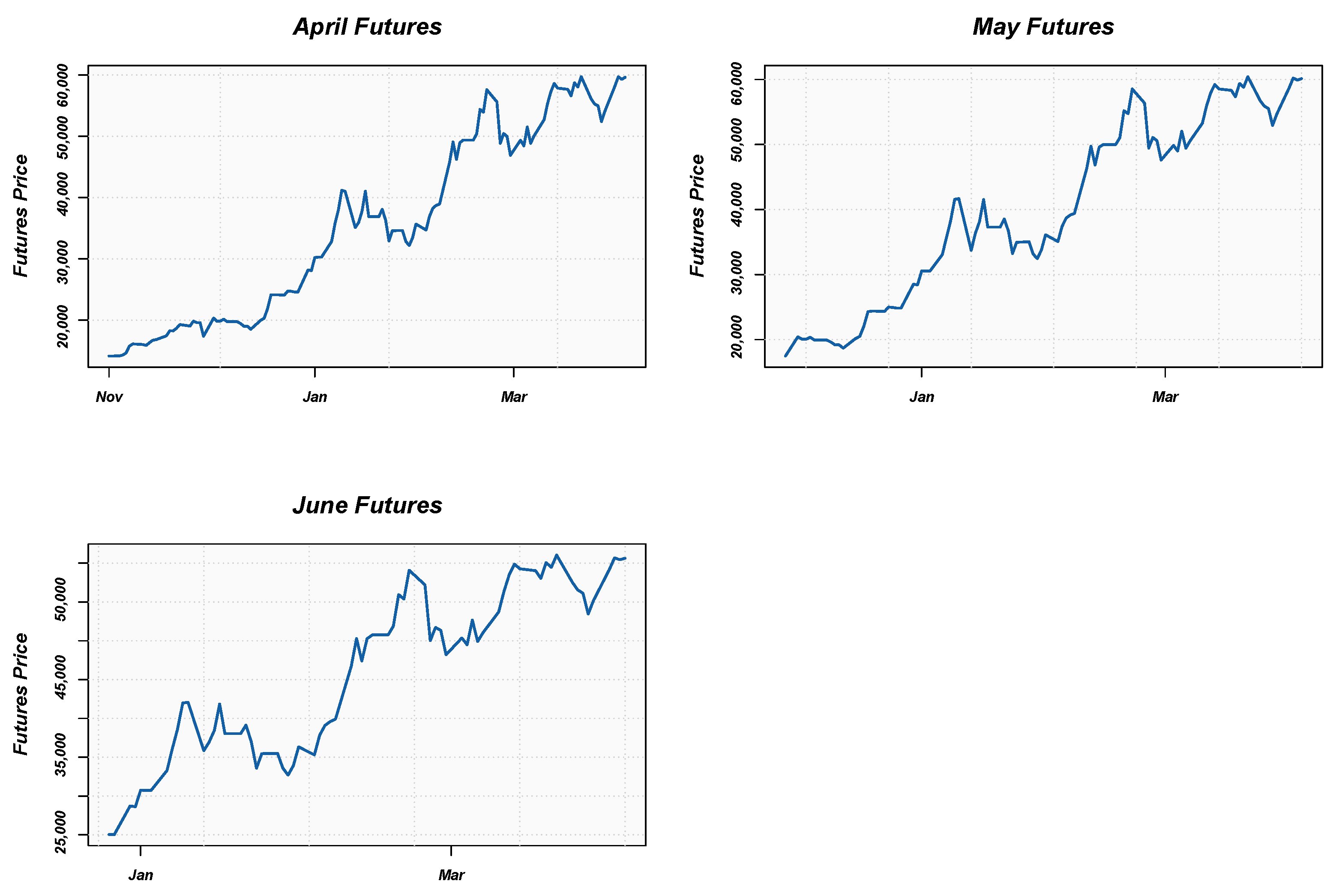
In this section, the empirical results are presented and discussed. In this study, daily data1 from 30 October 2020 to 1 April 2021 were used. The expiry dates of the Bitcoin futures prices are as follows: 30 April 2021, 28 May 2021, and 25 June 2021. The Bitcoin futures prices and returns are plotted in Figure 1 and Figure 2 below.
It is clear from the above that Bitcoin futures prices are trended. Furthermore, the returns show signs of volatility clustering, which is consistent with the typical stylised facts of financial returns (McNeil et al. 2015).
The descriptive statistics of the Bitcoin futures returns are reported in Table 1 below.
The descriptive statistics indicate that the conditional expectation of the returns is close to zero, the returns are not normally distributed, and the returns also show signs of leptokurtosis. This is consistent with the stylised facts of financial returns (McNeil et al. 2015).
The estimated parameters (maximum-likelihood) and information criteria of the symmetric and asymmetric HN model applied to Bitcoin futures returns are reported in Table 2 and Table 3 below.
The AIC indicates that the symmetric time-varying volatility model is a better fitting model. This is consistent with previous findings in the literature (see, e.g., Venter and Maré 2020; Conrad et al. 2018; Dyhrberg 2016). In addition to the AIC, a likelihood ratio test is also used to compare the estimated symmetric and asymmetric models. The test statistic of the likelihood ratio test for each expiry is reported in Table 4 below:
We do not reject the null hypothesis for each expiry (Held and Sabanés Bové 2014), which is also in favor of the symmetric HN model.
The futures option prices of the two models and market prices2 (scaled by the relevant futures price) are plotted in Figure 3 below. Furthermore, the pricing performance metrics of the two models applied to different futures are outlined in Table 5, Table 6 and Table 7.
It is clear that similar European futures option prices are obtained when the different models are compared. The models produce reasonable prices compared to market prices. The RMSE and MAE of the symmetric HN model are slightly lower compared to the asymmetric HN model.
The performance metrics of the two models are similar. Therefore, to determine whether the predictive accuracy of the two models are the same, the test by Diebold and Mariano (1995) was applied. The test statistic for each expiry is reported in Table 8 below:
The null hypothesis of the test is that the symmetric and asymmetric HN model have the same accuracy, and the alternative hypothesis is that the symmetric model outperforms the asymmetric model. The Diebold–Mariano test indicates that the symmetric model outperforms the asymmetric model for options that expire in April and May, but the predictive accuracy of the models is the same for options that expire in June.
Based on the pricing performance of univariate options, the symmetric HN GARCH process is used for the pricing of short-dated spread options on Bitcoin futures. For the CCC-GARCH model, no additional parameters need to be estimated. The additional parameters of the DCC-GARCH model are reported in Table 9 below:
The CCC-GARCH and DCC-GARCH models are compared using a likelihood ratio test. The value of the test statistic is −3.8 × 10, which is insignificant. Hence, we do not reject the null hypothesis, which is in favour of the CCC-GARCH model. Therefore, the CCC-GARCH model is used for the pricing of Bitcoin futures spread options.
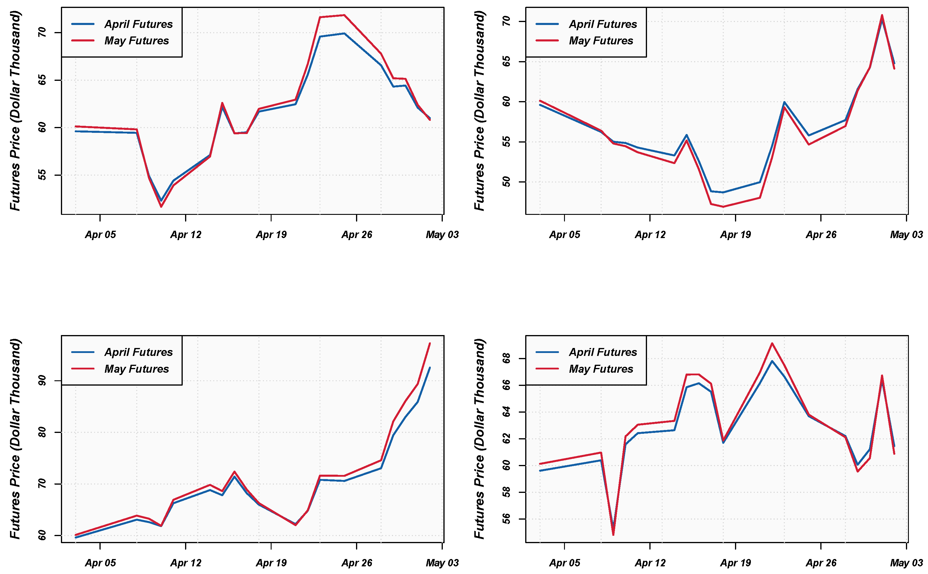
As mentioned previously, Bitcoin futures are highly correlated. To illustrate this concept, risk-neutral sample paths are illustrated in Figure 4 below.
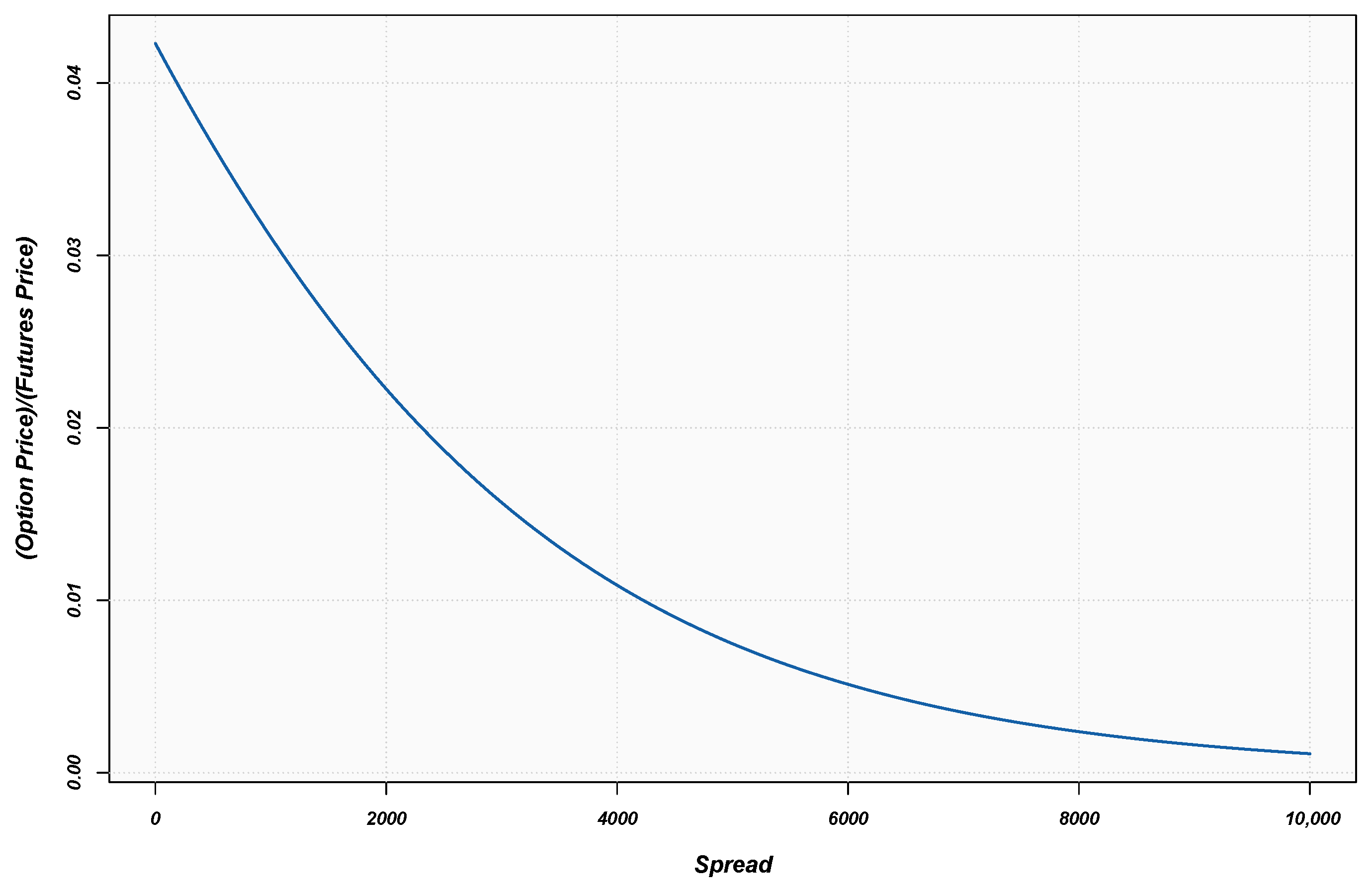
The sample paths are consistent with expectations. CCC-GARCH spread option prices (scaled by the April futures prices) are plotted in Figure 5 below. The spread option is based on the difference between the April and May futures prices, with an expiry date of 18 April 2021.
Spread options on Bitcoin futures do not actively trade and, therefore the model prices cannot be compared to market prices.
5. Conclusions
Bitcoin futures options were launched in the first quarter of 2020. GARCH modelling of Bitcoin returns and Bitcoin option pricing is well documented in the literature. However, the pricing of Bitcoin futures options in a GARCH framework has not been considered. In addition, a methodology for price discovery of multivariate options on Bitcoin futures has not been developed.
In this study, Bitcoin futures options were priced using the Heston–Nandi futures option pricing model (Li 2019a). The empirical results show that the symmetric Heston–Nandi model is a better-fitting model, which is consistent with previous studies that focused on Bitcoin spot return dynamics. The pricing performance metrics show that the Heston–Nandi model produces reasonable Bitcoin option prices, and that the symmetric Heston–Nandi model also produces more accurate option prices compared to market prices for two out of the three expiry dates considered.
In addition to the pricing of univariate Bitcoin futures options, the work by Rombouts and Stentoft (2011) was also extended to the pricing of multivariate futures options. The model was applied to Bitcoin futures spread options. The model produces reasonable spread option prices. However, spread options on Bitcoin futures do not actively trade. Therefore, the model prices cannot be compared to market prices.
The empirical results show that the symmetric Heston–Nandi model is more accurate in most cases. This implies that the symmetric model is a better choice when pricing exotic options (univariate) and other illiquid derivatives written on Bitcoin futures. Furthermore, the multivariate GARCH analysis showed that the CCC-GARCH model is more appropriate (based on historical data) when pricing multivariate Bitcoin futures options. Hence, the symmetric Heston–Nandi model and CCC-GARCH model can serve as a basis for pricing and risk measurement (quantifying market risk and capital calculations) of Bitcoin futures options.
Areas for future research include the use of skewness and kurtosis in the Heston–Nandi futures model (see e.g., Christoffersen et al. 2006) applied to univariate Bitcoin futures options, and the use of different multivariate GARCH processes (e.g., BEKK) applied to multivariate Bitcoin futures options. Furthermore, the hedge performance of the Heston–Nandi model applied to univariate and multivariate Bitcoin futures options should also be considered.
Author Contributions
Conceptualization, P.J.V. and E.M.; methodology, P.J.V.; software, P.J.V.; validation, E.M.; formal analysis, P.J.V.; investigation, P.J.V.; data curation, P.J.V.; writing—original draft preparation, P.J.V.; writing—review and editing, E.M.; visualization, P.J.V.; supervision, E.M.; project administration, E.M. Both authors have read and agreed to the published version of the manuscript.
Funding
This research received no external funding.
Institutional Review Board Statement
Not applicable.
Informed Consent Statement
Not applicable.
Acknowledgments
The authors would like to thank the editor and anonymous referees for their insightful comments and suggestions that helped improve the manuscript considerably.
Conflicts of Interest
The authors declare no conflict of interest.
| 1. | The dataset was obtained from the Thomson Reuters Datastream databank. |
| 2. | The market prices were obtained from CME Group. |
References
- Abraham, Rebecca. 2020. The role of investor sentiment in the valuation of bitcoin and bitcoin derivatives. International Journal of Financial Markets and Derivatives 7: 203–23. [Google Scholar] [CrossRef]
- Alexander, Carol, and Daniel F. Heck. 2020. Price discovery in Bitcoin: The impact of unregulated markets. Journal of Financial Stability 50: 100776. [Google Scholar] [CrossRef]
- Baur, Dirk G., and Brian M. Lucey. 2010. Is gold a hedge or a safe haven? An analysis of stocks, bonds and gold. Financial Review 45: 217–29. [Google Scholar] [CrossRef]
- Bharadwaj, Vishal. 2021. Growing Crypto Derivatives Market in India and the Government Regulations around it. European Journal of Molecular & Clinical Medicine 7: 3708–15. [Google Scholar]
- Chen, Yimiao, and Leh-Chyan So. 2020. New Insights from the Bitcoin Futures Market. Modern Economy 11: 1463. [Google Scholar] [CrossRef]
- Christoffersen, Peter, Steve Heston, and Kris Jacobs. 2006. Option valuation with conditional skewness. Journal of Econometrics 131: 253–84. [Google Scholar] [CrossRef] [Green Version]
- Clark, Iain J. 2014. Commodity Option Pricing: A Practitioner’s Guide. Hoboken: John Wiley & Sons. [Google Scholar]
- Conrad, Christian, Anessa Custovic, and Eric Ghysels. 2018. Long- and short-term cryptocurrency volatility components: A GARCH-MIDAS analysis. Journal of Risk and Financial Management 11: 23. [Google Scholar] [CrossRef]
- Diebold, Francis X., and Robert S. Mariano. 1995. Comparing predictive accuracy. Journal of Business and Economic Statistics 13: 253–65. [Google Scholar]
- Duan, Jin-Chuan, and Stanley R. Pliska. 2004. Option valuation with co-integrated asset prices. Journal of Economic Dynamics and Control 28: 727–54. [Google Scholar] [CrossRef]
- Dyhrberg, Anne Haubo. 2016. Bitcoin, gold and the dollar—A GARCH volatility analysis. Economic Letters 16: 85–92. [Google Scholar] [CrossRef] [Green Version]
- Engle, Robert. 2002. Dynamic conditional correlation: A simple class of multivariate generalized autoregressive conditional heteroskedasticity models. Journal of Business & Economic Statistics 20: 339–50. [Google Scholar]
- Fang, Libing, Elie Bouri, Rangan Gupta, and David Roubaud. 2019. Does global economic uncertainty matter for the volatility and hedging effectiveness of Bitcoin? International Review of Financial Analysis 61: 29–36. [Google Scholar] [CrossRef]
- Fassas, Athanasios P., Stephanos Papadamou, and Alexandros Koulis. 2020. Price discovery in bitcoin futures. Research in International Business and Finance 52: 101116. [Google Scholar] [CrossRef]
- Heston, Steven L., and Saikat Nandi. 2000. A closed-form GARCH option valuation model. The Review of Financial Studies 13: 585–625. [Google Scholar] [CrossRef]
- Francq, Christian, and Jean-Michel Zakoian. 2019. GARCH Models: Structure, Statistical Inference and Financial Applications. Hoboken: John Wiley & Sons. [Google Scholar]
- Held, Leonhard, and Daniel Sabanés Bové. 2014. Applied Statistical Inference. Berlin/Heidelberg: Springer. [Google Scholar]
- Jalan, Akanksha, Roman Matkovskyy, and Saqib Aziz. 2020. The Bitcoin options market: A first look at pricing and risk. Applied Economics 53: 1–16. [Google Scholar]
- Li, Bingxin. 2019a. Option-implied filtering: Evidence from the GARCH option pricing model. Review of Quantitative Finance and Accounting 54: 1–21. [Google Scholar] [CrossRef]
- Li, Bingxin. 2019b. Pricing dynamics of natural gas futures. Energy Economics 78: 91–108. [Google Scholar] [CrossRef]
- Mahringer, Steffen, and Marcel Prokopczuk. 2015. An empirical model comparison for valuing crack spread options. Energy Economics 51: 177–87. [Google Scholar] [CrossRef]
- McNeil, Alexander J., Rüdiger Frey, and Paul Embrechts. 2015. Quantitative Risk Management: Concepts, Techniques and Tools, Revised Edition. Princeton: Princeton University Press. [Google Scholar]
- Plakandaras, Vasilios, Elie Bouri, and Rangan Gupta. 2021. Forecasting Bitcoin Returns: Is there a Role for the US–China Trade War? Journal of Risk 23: 1–17. [Google Scholar]
- Rombouts, Jeroen VK, and Lars Stentoft. 2011. Multivariate option pricing with time varying volatility and correlations. Journal of Banking & Finance 35: 2267–81. [Google Scholar]
- Shahzad, Syed Jawad Hussain, Elie Bouri, David Roubaud, Ladislav Kristoufek, and Brian Lucey. 2019. Is Bitcoin a better safe-haven investment than gold and commodities? International Review of Financial Analysis 63: 322–30. [Google Scholar] [CrossRef]
- Siu, Tak Kuen, and Robert J. Elliott. 2021. Bitcoin option pricing with a SETAR-GARCH model. The European Journal of Finance 27: 564–95. [Google Scholar] [CrossRef]
- Venter, Pierre J., and Eben Maré. 2020. GARCH Generated Volatility Indices of Bitcoin and CRIX. Journal of Risk and Financial Management 13: 121. [Google Scholar] [CrossRef]
- Venter, Pierre J., Eben Maré, and Edson Pindza. 2020. Price discovery in the cryptocurrency option market: A univariate GARCH approach. Cogent Economics & Finance 8: 1803524. [Google Scholar]
- Wang, Tianyi, Yiwen Shen, Yueting Jiang, and Zhuo Huang. 2017. Pricing the CBOE VIX futures with the Heston–Nandi GARCH model. Journal of Futures Markets 37: 641–59. [Google Scholar] [CrossRef]
Figure 1.
Bitcoin futures.

Figure 2.
Bitcoin futures returns.
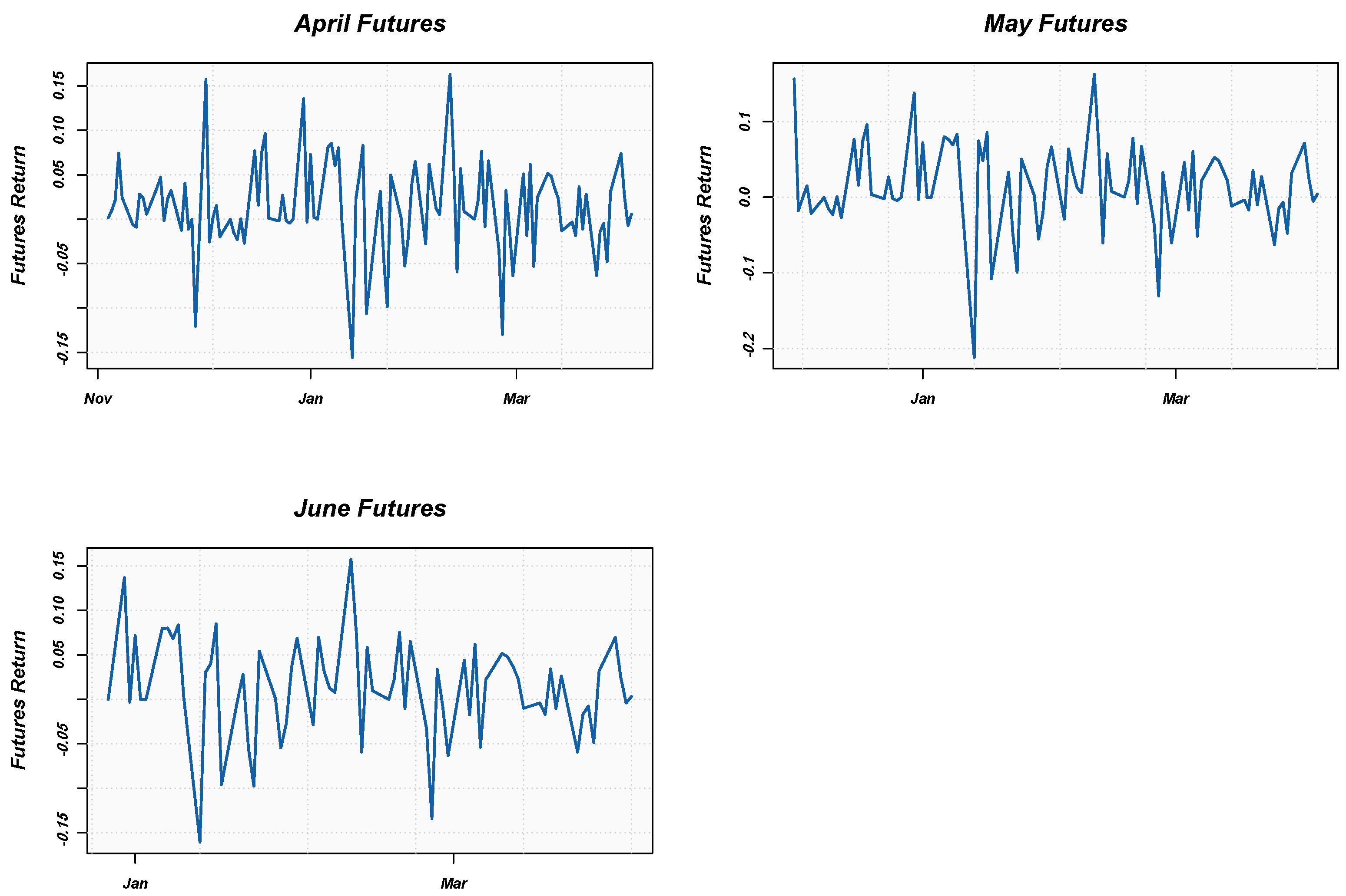
Figure 3.
Bitcoin futures option prices.
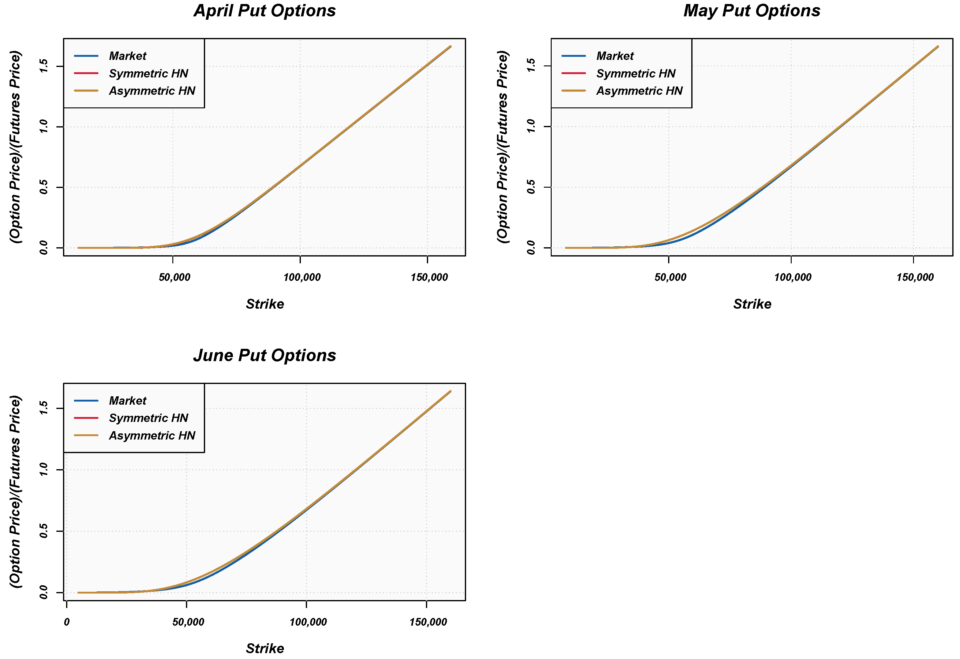
Figure 4.
Bitcoin futures sample paths.

Figure 5.
Bitcoin futures spread option prices.


Table 1.
Descriptive statistics: Bitcoin futures returns.
| April | May | June | |
|---|---|---|---|
| Mean | 0.0132 | 0.0139 | 0.0126 |
| Median | 0.0057 | 0.0038 | 0.0112 |
| Maximum | 0.1631 | 0.1626 | 0.1578 |
| Minimum | −0.1557 | −0.2118 | −0.1605 |
| Std. Dev. | 0.0517 | 0.0572 | 0.0563 |
| Skewness | −0.2318 | −0.5091 | −0.4326 |
| Kurtosis | 4.6279 | 5.3923 | 3.9755 |
| Jarque-Bera | 13.0122 | 25.0679 | 4.9587 |
| Probability | 0.0015 | 0.0000 | 0.0838 |
| Observations | 109 | 89 | 70 |
Table 2.
Symmetric HN parameters.
| April | May | June | |
|---|---|---|---|
| 5.2100 | 4.2970 | 4.0490 | |
| 0.0024 | 0.0030 | 0.0028 | |
| 2.0 × 10 | 3.5 × 10 | 3.2 × 10 | |
| 2.3 × 10 | 0.0685 | 0.0930 | |
| AIC | −4.1841 | −3.7271 | −3.2558 |
Table 3.
Asymmetric HN parameters.
| April | May | June | |
|---|---|---|---|
| 5.0020 | 4.2970 | 4.0490 | |
| 0.0023 | 0.0030 | 0.0028 | |
| 2.3 × 10 | 3.5 × 10 | 3.5 × 10 | |
| 3.4 × 10 | 0.0671 | 0.0927 | |
| 16.1600 | 0.3934 | 0.0986 | |
| AIC | −2.1870 | −1.7271 | −1.2558 |
Table 4.
Likelihood ratio test (HN).
| Expiry | Test Statistic |
|---|---|
| April | 1.2856 |
| May | 2.8 × 10 |
| June | −2.1× 10 |
Table 5.
April Performance Metrics.
| Symmetric HN | Asymmetric HN | |
|---|---|---|
| RMSE | 669.6865 | 724.2534 |
| MAE | 496.0976 | 533.5693 |
Table 6.
May Performance Metrics.
| Symmetric HN | Asymmetric HN | |
|---|---|---|
| RMSE | 1302.6712 | 1302.6727 |
| MAE | 1092.2221 | 1092.2235 |
Table 7.
June Performance Metrics.
| Symmetric HN | Asymmetric HN | |
|---|---|---|
| RMSE | 1149.2917 | 1149.2875 |
| MAE | 1018.2780 | 1018.2741 |
Table 8.
Diebold–Mariano test.
| Expiry | Test Statistic |
|---|---|
| April | −2.5072 * |
| May | −3.3034 * |
| June | 4.0599 |
* Denotes significance at a 1% level.
Table 9.
DCC-GARCH estimated parameters
| Estimated Parameter | |
|---|---|
| 1.4 × 10 | |
| 0.5657 |
Publisher’s Note: MDPI stays neutral with regard to jurisdictional claims in published maps and institutional affiliations. |
© 2021 by the authors. Licensee MDPI, Basel, Switzerland. This article is an open access article distributed under the terms and conditions of the Creative Commons Attribution (CC BY) license (https://creativecommons.org/licenses/by/4.0/).
Share and Cite
MDPI and ACS Style
Venter, P.J.; Maré, E. Univariate and Multivariate GARCH Models Applied to Bitcoin Futures Option Pricing. J. Risk Financial Manag. 2021, 14, 261. https://doi.org/10.3390/jrfm14060261
AMA Style
Venter PJ, Maré E. Univariate and Multivariate GARCH Models Applied to Bitcoin Futures Option Pricing. Journal of Risk and Financial Management. 2021; 14(6):261. https://doi.org/10.3390/jrfm14060261
Chicago/Turabian StyleVenter, Pierre J., and Eben Maré. 2021. "Univariate and Multivariate GARCH Models Applied to Bitcoin Futures Option Pricing" Journal of Risk and Financial Management 14, no. 6: 261. https://doi.org/10.3390/jrfm14060261