A Double-Hurdle Model of Healthcare Expenditures across Income Quintiles and Family Size: New Insights from a Household Survey

Abstract

The decision-making processes and outcomes of male and female household heads differ due to gender-based differences in preferences. In this paper, we assess the impact of this heterogeneity on household healthcare consumption in Thailand. Past studies modeling healthcare expenditures using household survey data used a gender dummy variable in regression models to control for household gender headship at the household level. Due to the endogeneity and self-selection bias in the past modelling approach, we separately modeled health expenditures for male and female household head decision makers. Using a household dataset from an earlier work, this study finds, using the double-hurdle model with dependent errors, that out-of-pocket health care spending tends to behave like a necessity across the income quintiles, household sizes, and differently for the separately modeled household gender heads. Moreover, male and female headed households responded differently to a major economic shock when adjusting household healthcare spending.

1. Introduction and Literature Review

Studies of human behavior attribute male–female differences in consumption and investments (including human capital such as health and education) to gender-induced differences in preferences (Dittrich and Leipold 2014; Dohmen and Falk 2011; Swope et al. 2008). A burgeoning body of literature has investigated the household consumption or expenditure data of particular goods (e.g., tobacco, alcohol) or commodity groups (e.g., food, recreation) by incorporating economic and demographic dimensions, among others. However, with particular reference to out-of-pocket (OOP) health care expenditure, to the authors’ knowledge, there are no studies that explicitly test the hypothesis that the slope, intercept effects, and elasticities of the various determinants of consumer expenditures differ across income ranges for male compared to female headed households, in any country, regardless of the economic development stage. The purpose of this replication study is to assess the differences that arise in healthcare consumption as a result of gender-specific preferences. While the spirit of the paper remains empirical, we also provide a theoretical framework and empirical strategy that both predict and account for these differences in preferences in the empirical process.

When estimating demand, controlling for gender-based variation in preferences is crucial. Female household headship is growing steadily due to favorable global trends among women including the broadened personal choices (freedom of education and work, immigration, pregnancy and abortions, type of work), economic empowerment, marital disruptions (divorce, widowhood and etc.), alternative family life-styles (e.g., adult male, rural-urban living choices) and socio-cultural traditions in some societies (Flatø et al. 2017; Liu et al. 2017). Headship of household is defined as the primary decision maker within the household and is not necessarily the chief wage earner. Women widely perceived as the main brokers of health and education in the household. They tend to also channel greater shares of common resources to health, food, and nutrition that promote general welfare and well-being of others in the household (Duflo 2012). Transition in women’s role and these trends have important public policy implications (Doepke and Tertilt 2009).

Women have empirically revealed preferences that treat human capital inputs very differently from men. This is consistent with heterogeneous preferences in consumption; exhibiting gender bias1 specifically in healthcare (Chiappori et al. 2009; Schünemann et al. 2017). The preference of female heads to allocate a relatively greater share of household resources for healthcare is theoretically attributable to others’ utilities entering into her own utility function (Onah and Horton 2018). This is perhaps through altruism (Said et al. 2020), inequality aversion (He and Villeval 2017), or reciprocity (Çelen et al. 2017). Additionally, more risk averse female heads may be less likely to gamble with the health of other household members. Using economic experiment data, Croson and Gneezy (2009) tested the impacts of preference parameters, including self-selection and learning in men and women. They find that women are more risk averse, and their social preferences are more situational and malleable. Male and female heads also tend to interpret health risks differently (Flory et al. 2018). This diversity in risk assessment is indicative of greater differences in underlying preferences regarding necessity. When decisions are made at the household level, as in our study, gender-specific preferences concerning risk and need affect more than one individual’s welfare.

In general, medical care, when consumed, is a necessity (Dunn 2016). More than 150 million people globally, mostly in poor households, suffer financial catastrophe annually due to high OOP health expenditures (Xu et al. 2007). Many households in developing countries spend at least half of their monthly current income on health (Grigoli and Kapsoli 2018). In Mexico, for instance, 46.18 percent of the remittances of their nationals are for health care expenses (Hadad et al. 2013). Preferences over health differ not only by gender but also by income. Household OOP outlays, the major source of personal healthcare financing in most developing countries, can heavily burden poor households (Jakovljevic et al. 2017). They may accelerate health status decline if personal financial woes are protracted in the absence of reliable public assistance or an effective regulatory authority (Arthur and Oaikhenan 2017). OOP payments are the primary means of financing health care in much of Asia, where the ratio of OOP to total household health expenditure ranges from 30 to 82 percent (Van Doorslaer et al. 2007) and is higher for poor than rich families. In developing countries, low care quality may lead to wasteful interventions for which patients must pay out-of-pocket. The importance of OOP payments cannot be understated, since the acquired health status directly augments utility and is used to generate earnings or wealth in a life-cycle context (Galama and Van Kippersluis 2019). As a rapidly developing economy, healthcare is a critical basic need in Thailand as a healthier and more productive population base is a catalyst for generating a sustainable economic growth (Moore and Donaldson 2016).

The need to account for healthcare demand behavior consistent with the permanent income concept is fundamental in developing countries, where savings and assets affect the speed at which the nation converges to long-run steady-state macroeconomic development (a la Solow). In asking if income matters, two types of evidence are relevant: the relation of income to health between and within countries, and the relation of income inequality to health. Further, there are also two related debates: the degree to which the apparent relation of income to health should be thought of as a question of poverty or (inequality) and the role of material and psychosocial factors in generating in-equalities in health. There is an extensive literature that notes on the evidence that health can affect income, but that it is not the major explanation of the link between income and health. This has been dealt with in other related studies (Deaton and Paxson 1998; Ecob and Smith 1999; Frijters et al. 2005; Marmot 2002; Subramanian and Kawachi 2006). The choices households in developing countries make regarding capital accumulation based upon their savings and asset base, particularly those comprising health capital, should not be ignored. Yet, inclusion of long-term income that expands household resource flows is novel in health expenditure research (Engström and Hagen 2017; Okunade et al. 2018). Few past studies include wealth or assets as a major determinant of total health expense levels2. In developing countries such as Thailand, given the fragility of safety nets for necessities such as medical care the inclusion of assets is critical for relaxing household budget constraints. In such areas poor families may divest human and physical capital, cut other essential consumption, liquidate assets, and incur debts to defray necessary out-of-pocket costs of critical healthcare (Aregbeshola and Khan 2018; Rieger et al. 2017).

This study contributes materially to the existing literature on modeling household healthcare spending. First, we present a theoretical foundation and an empirical strategy to account for unobserved, heterogeneous preferences in line with empirical realities of healthcare consumption (zero inflation data and healthcare as a necessity) in the developing country context. Revisiting an earlier work (Okunade et al. 2010) and using a replication strategy, we estimate a double-hurdle model of the determinants of out-of-pocket total health expenditures based on household survey data of the developing country. Second, relying on heterogeneous preferences of male compared with female household heads in healthcare consumption and statistical test verification, separate dependent-error double-hurdle models are estimated to more cleanly capture effects of household-head genders, for small and large household groups, within and across income quintiles. Moreover, we test for income and asset elasticity variations across the household gender types, income quintiles, and household sizes. To our knowledge, this is a novel effort. The contributions of our work are insightful for improving econometric models of household healthcare spending in the developing country context.

This paper proceeds as follows. The next section is on the two-stage decision theory underlying health care consumption. The empirical strategy and the data are discussed in the sections that follow. The final two sections of the study focus on the empirical results, implications, and conclusions.

2. Health Capital Model of Health Goods/Services Consumption

Two-stage empirical strategies are widespread in health economics (Terza et al. 2008). Normally, stage one is used to control for market selection and the other to control for the quantity of healthcare consumed. These models are well motivated by most healthcare data. Indeed, data reveal that individuals purchasing healthcare in markets often behave as if the goods and services are necessities. Yet, the data sets are often zero-inflated, even to the order of 30 percent of the sample. That is, some consumers choose not to consume a good that behaves as technical necessity in the first place. How is this possible?

Theoretical frameworks for testing the heterogeneity of preferences for health care exist, as do ones incorporating agent (e.g., household) level decisions and risk aversion. However, none answer the necessity-zero-consumption question in a way that motivates the explicit two-stage framework in empirical work. This section offers a compelling foundation that naturally accounts for agent decisions, risk, and heterogeneous preferences both across observations and across market decisions for the same consumer’s observation. In doing so, the logic motivates a very general body of two-stage models for estimation of demand under the paradox of necessity and non-consumption3.

Let consumers hold preferences over multiple goods, one being their stock of health capital. Health enters $U(X,k)$, as the preference function, where $k$ represents the stock of health capital and $X$, is a composite of all other goods4. Individuals maximize $U(X,k)$, with respect to $k$, under normal permanent income budget considerations to set $k^{*}$, the optimal level of health capital desired. It should be noted that the consumers own valuation of health, risk preferences, concepts of need, the advice of agents (such as physicians), and any other diverse factors set $k^{*}$. Since $k^{*}$ is not a direct commodity it cannot be purchased in a market; normal demand for $k^{*}$ is not applicable. Thus, after setting $k^{*}$ the individual is forced to derive demand for health capital inputs.

Let $k^{*}=f(h,c)$ define a health capital contribution function where $h$ is healthcare and $c$ is a composite of all other contributors to a consumer’s level of health. Note that once $k^{*}$ exists, $k$, now has inputs and is similar to a production function. Here we make an assumption that an individual’s health receives momentary shocks. For any given period with $k_0$, health capital, there will be a probability that $k_0<k^{*}$, the maximizing level of health capital. Since health directly enters the preference function, $k_0<k^{*}$, it is equivalent to a negative shock to utility and preferences are no longer maximized subject to the permanent income budget constraint. Thus, when $k_0\ge k^{*}$, preferences are maximized and there is no incentive to contribute to $k$. For $k_0<k^{*}$, the consumer must demand inputs to $k$ until $k_0$ converges back to $k^{*}$. Because $h$ is an input, consumer demand for $h$ is derived by an expenditure minimization process. The resultant demand for $h$ is analogous to factor demand in producer theory and is a compensated demand in $k^{*}$. This is the observed demand for healthcare.

Two observations arise from this logic. First, $h$ is a compensated demand in $k^{*}$. Unless other health capital inputs are very close substitutes, the individual only seeks to minimize the cost of obtaining $k^{*}$ health by purchasing $h$ healthcare. Thus, demand for $h$ has little or no substitution effect and behaves like a technical necessity. Second, whenever $k_0\ge k^{*}$ demand for $h$ is zero. This can occur even when $k$ enters significantly into the preference function, or when maximum utility requires a lower $k^{*}$.

The health care demand decision then has two-parts. The first decision governs whether the consumer enters the market for health capital input $h$, that is whether $k_0<k^{*}$. This stage controls for heterogeneity in preferences over $k$ and diverse (even unknown) $k_0$. The second decision governs the expenditure minimizing choices for the $k$ inputs, and thus healthcare $h$, given that $k^{*}$ must be ultimately achieved. This theoretical foundation directly motivates a two-stage empirical approach. It predicts that demand for healthcare will behave like a necessity. It also predicts that the data will observe zero-consumption.

3. Empirical Strategy

The logic of the model outlined above requires an empirical strategy controlling for diversity in preferences in both the choice to consume and the choice of how much to consume. Returning to the consumer’s relevant choice for healthcare market entrance. Let the stock of health capital follow a stochastic process in order that it may receive random shocks over time. Then, for a given period, there exists a probability for the event that initial health capital stock $k_0$ is below the desired level:

$$\mathrm{Pr}(k_0<k^{*}),$$

(1)

where (1) follows some probability distribution with parameters $(k^{*},k_0)$, and is the probability that health falls below the desired level. Equation (1) is different for each consumer. The distribution of (1) is unknown, as are all preferences, units, and magnitudes necessary for calculating the associated probability. Dividing by $k^{*}$ achieves an intuitive normalization:

$$\mathrm{Pr}(\frac{k_0}{k^{*}}<1).$$

(2)

Now everything can be interpreted in terms of ratios and all of the units and magnitudes that differ across individuals are removed. Additionally, in (2) all pertinent information on diverse preferences is carried to the probability space through $k^{*}$, and all information on initial stock of health is carried through $k_0$. In other words, controlling for differences in (2) across consumers is equivalent to controlling for heterogeneity in their preferences, risk, and health status. Equation (2) is still unobservable. For most data, we are only able to observe the probability that a consumer enters the market:

$$\mathrm{Pr}(E=e),$$

(3)

where (3) has some observable probability distribution for a market entrance outcome $e$ taking the values (0, 1). Per the theoretical model, consumers will enter the market if and only if their health stock falls below the preference maximizing level, $(k_0<k^{*})$. Thus:

$$\mathrm{Pr}(E=1)=\mathrm{Pr}(k_0<k^{*})=\mathrm{Pr}(\frac{k_0}{k^{*}}<1).$$

(4)

With this association, unobservable heterogeneity in preferences is transformed to observable heterogeneity in the probability of market entrance. All of the information in (2), even gender-specific preferences, health status, and risk aversion, is obtained by controlling for (3)’s probabilities in the empirical exercise. After choosing to enter the market, $h_i$ is the healthcare expenditure and $E_i$ is the market entrance outcome for the $i^{th}$ consumer.5 As the model predicts, data with zero inflation renders $\mathrm{Pr}(E_i=0)$ non-zero and non-trivial. This restricts the empirical estimation of total expenditure on healthcare to:

$$E[h_i|h_i>0]={\beta }_i{X}_i+{\epsilon }_i$$

(5)

where $\mathrm{Pr}(h_i>0)$ is equivalent to $\mathrm{Pr}(E_i=1)$, ${\beta }_i{X}_i$ is a vector of covariates such as income, and ${\epsilon }_i$ is an error term for the $i^{th}$ consumer. In words, given that a consumer’s preferences over $k^{*}$ and health status $k_0$ have compelled them to enter the market, one can empirically estimate their expected expenditure for healthcare as a function of other determinants. There are many options for two-stage estimation of (5). We desire as much flexibility as possible at each stage to ensure unbiased results.

An ideal specification for such flexibility is a double hurdle model with dependent errors. The double hurdle model is a generalization of the popular Tobit model in which the first stage probit equation is allowed to have separate covariates and a different decision structure from the second stage’s estimation of the coefficients. Formally, for the latent dependent variable $h_i$ the data only observes:

$$h_i=d_i\cdot h_i^{*},$$

(6)

where d_i is the dichotomous participation decision and $h_i^{*}$ is the post-entrance healthcare spending. The double hurdle model decomposes ${\epsilon }_i$ from (5) into $u_i$ and $v_i$ distinct (but possibly correlated) errors for each stage. The $d_i$ hurdle for obtaining $\left\{\mathrm{Pr}(\frac{k_0}{k^{*}}<1)=\mathrm{Pr}(E_i=1)=\mathrm{Pr}(h_i>0)\right\}$ is:

$$d_i=\left\{\begin{array}{cc}1& if{w}_i>0\\ 0& otherwise\end{array}\right\},w_i={\alpha }_i^{\prime }{z}_i+u_i{u}_i\sim N(0,1)$$

(7)

where the chance $d_i=1$ follows its own decision process $w_i$ with covariate structure ${\alpha }_i^{\prime }{z}_i$ and $u_i$ error term. Noting that $h_i=d_i\cdot h_i^{*}$ is only observed if $d_i=1$ $d_i=1$, the $h_i^{*}$ hurdle for estimating health expenditure is:

$$h_i^{*}=\left\{\begin{array}{cc}{h}_i& if{h}_i>0\\ 0& otherwise\end{array}\right\}{h}_i={\beta }_i^{\prime }{X}_i+v_i{v}_i\sim N(0,{\sigma }_i^2),$$

(8)

where ${\beta }_i^{\prime }{X}_i$ is the $i^{th}$ consumer’s covariate vector determining $h_i$ and $v_i$ is an error term. To allow dependence between the equations, $u_i$ and $v_i$ are assumed distributed bivariate normal with correlation $\rho$. With these parameters the double hurdle likelihood function for estimating (5) takes the form:

$$L={\displaystyle \prod _0\left[1-\Phi ({\alpha }_i^{\prime }{z}_i,{\beta }_i^{\prime }{X}_i,\rho )\right]}x{\displaystyle \prod _{+}\Phi \left[\frac{{\alpha }_i^{\prime }{z}_i+\frac{\rho }{{\sigma }_i}(h_i-{\beta }_i^{\prime }{X}_i)}{\sqrt{1-{\rho }^2}}\right]}\frac{1}{{\sigma }_i}\varphi \left[\frac{h_i-{\beta }_i^{\prime }{X}_i}{{\sigma }_i}\right],$$

(9)

where Φ and ϕ denote the normal cumulative distribution and density functions. In words, (9) estimates a probit first stage to account for zero-consumption and then assesses the conditional expectation for the total health expenditure $h_i$. The separate covariate structure ${\alpha }_i^{\prime }{z}_i$ gives flexibility to the first stage’s calculation of heterogeneous probabilities (and thus diverse preferences). The correlation coefficient $\rho$ allows the errors of each stage to better reflect correlation in preferences between the consumer’s decisions; $\rho$ also helps correct for omitted variables that influence the estimation.

4. Data and Empirical Model

Data used in econometric estimation come are from Okunade et al. (2010). The data consists of 98,632 household observations from four biennial waves of the nationally representative Socio-Economic Surveys SES), conducted biennially by the National Statistical Office (NSO, hereafter) in all 76 provinces of Thailand. The SES collects detailed household data on income, expenditure and consumption of commodities, changes in assets and liabilities, durable goods ownership, and information on household members including the gender. The sampling frame covers private, non-institutional households residing permanently in municipal and non-municipal areas (sanitary districts and villages). The data are cross-sections of randomly selected households in each round of the survey.6

The goal of this study goal is to investigate variation in total health expenditure as a result of diverse preferences arising under male and female household heads, income quintiles and household sizes. To better account for these differences, we model healthcare expenses under each preference set separately.7 We control for other socio-economic characteristics, demographics, and a one-time macroeconomic shock as determinants. The dependent variable, defined as real household OOP health care expenditure, combines private spending on medical supplies (e.g., traditional herbs and drugs, prescriptions, vitamins, condoms, medical care supplies and equipment), outpatient services, and inpatient medical services at public and private facilities.8 Theoretical determinants of health expenditure include consumer tastes and needs, socio-demographics, and economic resources.

One hypothesis tested here is that out-of-pocket household health expenditures are likely to decline as a share of income in a period of significant macroeconomic shock that occurred. If support is found, policy makers should rethink public health safety net designs to reduce population health decline during economic downturns. Past health expenditure studies also found a positive and statistically significant effect of current, measured, or absolute income (Lago-Peñas et al. 2013; Murthy and Okunade 2016), socio-demographic variables such as formal education (Aregbeshola and Khan 2018), age (Chi and Hsin 1999; Di Matteo 2005) and proximity to death (Howdon and Rice 2018).

The socio-demographic variables constructed include median household age, proximity to death of the oldest household member, household head education, and household head gender as proxies for tastes that influence healthcare demand.

Table 1. Descriptive Statistics.

Variable	Total Sample	Male Head	Female Head
Household out-of-pocket (OOP) health expenditure (in Baht)	351.05 (3242.29)	348.62 (1926.83)	357.86 (5434.22)
Log (OOP health expenditure)	3.48 (2.53)	3.52 (2.52)	3.39 (5.57)
Macroeconomic shock (0 = before 1997, 1 = after 1997)	0.49 (0.50)	0.48 (0.50)	0.51 (0.50)
Real monthly household income	13601.48 (21,980.85)	14126.16 (23,176.86)	12134.07 (18,143.85)
Real household income squared	6.68 × 108 (1.20 × 1010)	7.37 × 108 (1.30 × 1010)	4.76 × 108 (8.63 × 109)
Income quintile household size dummies a - 20th percentile with ≥5 household members - 40th percentile with ≥5 household members - 60th percentile with ≥5 household members - 80th percentile with ≥5 household members - 100th percentile with ≥5 household members	0.09 (0.285) 0.06 (0.240) 0.05 (0.22) 0.04 (0.20) 0.03 (0.16)	0.10 (0.30) 0.07 (0.25) 0.06 (0.23) 0.04 (0.21) 0.03 (0.17)	0.06 (0.24) 0.05 (0.21) 0.04 (0.19) 0.03 (0.18) 0.02 (0.14)
Region dummies b - Central - North - Northeast - South	0.25 (0.43) 0.22 (0.42) 0.28 (0.45) 0.17 (0.37)	0.24 (0.42) 0.23 (0.42) 0.29 (0.45) 0.17 (0.38)	0.29 (0.46) 0.22 (0.42) 0.26 (0.44) 0.14 (0.35)
Household head education dummies c - Some or complete secondary - Some or complete university	0.13 (0.34) 0.14 (0.34)	0.15 (0.35) 0.13 (0.34)	0.08 (0.28) 0.14 (0.35)
Household head gender is male	0.74 (0.44)	1.00 (0.00)	0.00 (0.00)
Median age	33.54 (15.27)	33.33 (14.92)	34.13 (16.18)
Median age squared	1357.85 (1245.69)	1333.22 (1204.79)	1426.73 (1351.17)
Proximity to death	21.72 (14.62)	21.88 (14.20)	21.28 (15.73)
Proximity to death squared	685.77 (689.32)	680.62 (651.34)	700.17 (785.70)
Wealth index	0.00 (1.00)	0.015 (1.00)	−0.043 (0.995)
Number of observations	98,632	72,654	25,978

Data Source: Thailand Socioeconomic Survey, 1994, 1996, 1998, 2000. Data means are calculated (standard errors in parentheses). ^a Omitted quintile categories for each quintile when household size equals 4 or less. ^b Omitted region category is Bangkok metropolis. ^c Omitted schooling group is household heads with no formal education or some or complete primary.

contains descriptive statistics of the full sample and the male–female subsamples. Of the 98,632 total household observations, 73.7% (72,654) are male-headed and the rest female-headed. This distribution is similar to Flatø et al. (2017) and consistent with the rising importance and recognition of the growth in female-headed households in economic literature on gender, health inequality, and development (Liu et al. 2017). Specifically, female household heads generally display different sociological and economic characteristics from males and these differences have major implications for designing effective public policy and programmatic interventions (Joshi Rajkarnikar and Ramnarain 2020). In this regard, male-headed Thai households earned higher real incomes but spent less on OOP health expenses than their female-headed counterparts. There is little variation in the proportion of male and female heads across household sizes, income quintiles, and geographic areas. In comparison with male heads, the median age of female heads is older and the negative asset index for the typical female-headed household suggests liabilities in the ownership of fixed assets in a culture of male-dominance.

Since household utility is assumed to be derived from the welfare, including health of the constituent members, age is measured as median age. Proximity to death is calculated as the difference between age of the oldest household member and gender-based life expectancy. Squared terms of continuous variables are included to incorporate potential nonlinearities. Education dummy variables denote household heads with some or complete secondary education and those with some or complete university. The omitted education category is elementary-level or below. Regional dummies (Bangkok metropolis is the base) capture heterogeneous region-specific differences in access to medical facilities, demand-supply imbalances, and any other spatial variations affecting health care prices and consumption.

A consumer’s physical and human assets influence the ability to earn wages and help construct anticipated lifetime income. Households may liquidate some assets to relax tight budget constraints when purchasing medical care. Therefore, in addition to measuring real disposable income at a point in time, a core determinant of consumption is household wealth (Pistaferri 2001). In our model a measure of household ownership of durable goods (air conditioner, motorbike, car, television, etc.) is introduced as proxy for household wealth and used for calculating the ‘wealth index’ by the principal components analysis (Garin et al. 2018). Total monthly household income is wages and salaries plus non-farm and farming profit, transfer payments, property income, and other monthly receipts. Correlation of the wealth index and monthly income in pre 1994–1996 and post 1998–2000 economic shock eras is low across income quintiles. Thus, orthogonality of these determinants in the data design matrix suggests they represent separate and sufficiently independent dimensions of the household resource base. We unfortunately do not have data on health insurance. By controlling for differences in preferences and health capital stock that determine insurance coverage in the first place, the first stage of the model does control partially for the omission of insurance. Finally, certain private transfers such as those from social capital networks (extended families, friends) that contribute to household economic well-being are excluded here for lack of salient data. However, public transfer payments are included as a component of income. Our empirical specification of the second stage expenditure process takes the form:

$$Log(HOHEX{P}_i)=\beta i_{i0}+{\beta }_i{X}_i+v_i,$$

(10)

where $HOHEX{P}_i$ is the i^th household’s real OOP health expenditure indexed by income quintile, gender, and family size. X_i is a vector of model determinants (income, asset index, household head education, geographic region, etc.), and $v_i$ is the residual. Equation (10) is separately estimated for male and female household heads in each income quintile and for small and large households. The double hurdle strategy yields twenty models, each with the two equations.

5. Empirical Results and Implications

This paper models zero-inflated data; 28.45% of the 98,632 survey responded incurring zero OOP health expenditure for four waves of biennial national surveys.

Table 2. Descriptive Statistics of zero versus non-zero observed OOP health expenditures.

Variable	Observations with Non-Zero OOP	Observations with Zero OOP	Statistical Significance of Difference in Means d
Household out-of-pocket (OOP) health expenditure (in Baht)	490.64 (3824.15)	0.00 (0)	−21.49 ***
Log (monthly OOP health expenditure)	4.87 (1.5)	0.00 (0)	−550.00 ***
Macroeconomic shock (0 = before 1997, 1 = after 1997)	0.48 (0.50)	0.52 (0.50)	111.42 ***
Real monthly household income	13,392.18 (21,299.55)	14,127.86 (23,599.7)	4.74 ***
Real household income2	6.33 × 108 (1.10 × 1010)	7.57 × 108 (1.41 × 1010)
Income quintile household size dummies a 20th percentile with ≥5 in the household 40th percentile with ≥5 in the household 60th percentile with ≥5 in the household 80th percentile with ≥5 in the household 100th percentile with ≥5 in the household	0.10 (0.30) 0.07 (0.25) 0.055 (0.23) 0.04 (0.20) 0.03 (0.16)	0.07 (0.26) 0.05 (0.21) 0.04 (0.19) 0.04 (0.18) 0.03 (0.16)	174.74 *** 158.28 *** 108.35 *** 36.62 *** 6.50 **
Region dummies b Central North Northeast South	0.25 (0.43) 0.23 (0.42) 0.29 (0.45) 0.16 (0.37)	0.25 (0.43) 0.25 (0.41) 0.26 (0.43) 0.18 (0.38)	3.04 * 21.96 *** 120.20 *** 92.67 ***
Household head education dummies c Some or complete secondary Some or complete university	0.12 (0.32) 0.12 (0.32)	0.15 (0.36) 0.19 (0.39)	216.77 *** 874.25 ***
Household head gender is male	0.74 (0.44)	0.72 (0.45)	64.49 ***
Median age	33.68 (15.40)	33.18 (14.91)	−4.65 ***
Median age	1371.667 (1260.22)	1323.09 (1207.70)
Proximity to death	21.01 (14.45)	23.51 (14.9)	24.32 ***
Proximity to death	650.33 (664.92)	774.89 (739.72)
Wealth index	0.01 (1.00)	−0.01 (0.10)	−2.33 **
Number of observations	70,571	28,061

Data Source: Thailand Socioeconomic Surveys. Data means (standard errors in parentheses) are the authors’ calculations. ^a Omitted quintile categories for each quintile when household size equals 4 or less. ^b Omitted region category is Bangkok metropolis. ^c Omitted schooling group is household heads with no formal education or some or complete primary. ^d Symbols ***, **, and * denote statistical significance of the estimates at the 0.01, 0.05, and 0.10 levels respectively; Pearson χ² (t-statistics) hypothesis test results are reported for indicator (continuous) variables.

shows significant differences in mean data values for the zero out-of-pocket expenditure sub-sample compared with the non-zero OOP sub-sample. This reinforces the appropriateness of modeling OOP health care spending for Thailand using the double-hurdle framework. Moreover, of the 72,654 (25,978) male (female) headed household observations 27.8% (30.4%) is censored. Okunade et al. (2010) using the same dataset as this study, reported a highly significant and negative coefficient of the male household head gender dummy as a determinant of out-of-pocket health care spending.

Table 3. Double-Hurdle Regression Results (Total Sample), Household Data ^a.

	Male Head		Female Head		Elasticities
Variable	1st Stage	2nd Stage	1st Stage	2nd Stage	Male [Female]
Dependent variable: log (out-of-pocket health expenditure)
Constant	−0.008 (0.047)	5.53 *** (0.054)	−0.101 (0.070)	5.74 *** (0.085)
Dummy for economic shock (0 before 1997; 1 thereafter)	−0.091 *** (0.010)	−0.074 *** (0.013)	−0.066 *** (0.017)	−0.045 ** (0.022)
Dummy for consumption income quintile and family size b 20th percentile and family size of 5 members or more		−0.013 (0.023)		−0.060 (0.046)
40th percentile and family size of 5 members or more		0.068 *** (0.026)		0.061 (0.050)
60th percentile and family size of 5 members or more		0.198 *** (0.028)		0.179 *** (0.055)
80th percentile and family size of 5 members or more		0.312 *** (0.032)		0.371 *** (0.060)
100th percentile and family size of 5 members or more		0.671 *** (0.039)		0.592 *** (0.080)
Dummy for region c Central	0.143 *** (0.021)	−0.300 *** (0.028)	0.132 *** (0.033)	−0.406 *** (0.046)
North	0.172 *** (0.021)	−0.551 *** (0.028)	0.154 *** (0.034)	−0.659 *** (0.048)
Northeast	0.161 *** (0.020)	−0.611 *** (0.028)	0.198 *** (0.033)	−0.732 *** (0.047)
South	0.020 (0.021)	−0.400 *** (0.029)	0.057 (0.036)	−0.487 *** (0.051)
Dummy for education d Secondary	−0.146 *** (0.014)	0.189 *** (0.020)	−0.213 *** (0.030)	0.215 *** (0.044)
University	−0.236 *** (0.015)	0.432 *** (0.022)	−0.349 *** (0.024)	0.423 *** (0.040)
Median age	0.0006 (0.002)	−0.005 *** (0.002)	0.002 (0.002)	−0.009 *** (0.003)	0.062 [0.111]
Median age squared	0.00004 ** (0.00002)	0.0001 *** (0.00002)	0.00002 (0.00003)	0.0001 *** (0.00003)
Proximity to death	−0.0019 (0.001)	−0.006 *** (0.002)	−0.0007 (0.002)	−0.003 (0.002)	−0.146 [−0.054]
Proximity to death squared	0.00003 (0.00003)	−0.00002 (0.00003)	−0.00004 (0.00004)	−0.00008 (0.00005)
Wealth index		0.259 *** (0.007)		0.300 *** (0.011)	−0.011 [0.005]
Family Size (continuous- selection only)	0.184 *** (0.010)		0.151 *** (0.015)
Family Size squared (continuous- selection only)	−0.010 *** (0.001)		−0.009 *** (0.002)
No of observations	72,654		25,978
No of censored observations	20169		7892
Estimated$\rho$	−0.268 ***		−0.236 ***
Ln$\sigma$	0.373 ***		0.374 ***
Log-Likelihood function value	−134,904.1		−47,572.08
Wald${\chi }^2$test of Indep. Eqns. (p > chi-squared)	84.40 (0.0000)		17.52 (0.0000)

Source: Thailand Socioeconomic Survey, 1994, 1996, 1998, and 2000 (authors’ calculations). ^b Each quintile estimate is relative to same income quintile-small family cohort ^c Omitted region is Bangkok. ^d Omitted education group is household heads with no formal schooling and with some or complete elementary. ^a *** p > 0.01; ** p > 0.05 are significance levels.

presents household head gender-specific first (probit) and second (expenditure) stage regression estimates to probe deeper into the differential determinants of health expenses in male versus female headed households. The estimates confirm variation in the magnitudes and directions of the model determinants across household head genders. The highly significant Wald χ² test of independent errors across first and second stage decisions suggests rejection of the null. The statistical significance of the parameter estimate ρ further suggests the inappropriateness of assuming independence of the decision hurdles. That is, first and second stage decisions are dependent models (see, Table 3) and the reported standard errors are robust.

Interesting insights emerging from the first stage model estimates (Table 3) are as follows. First, the 1997 economic shock had a greater adverse impact on the decision to spend OOP on health care in male than female headed households, and the effect is highly significant for each gender. This is unlike the finding in (Klasen et al. 2015) which did not find a difference in the impact of economic shock between male and female-headed household as a group even though de jure female headed households are less affected. Males cut health expenses deeper than female heads in hard economic times. This tendency has implications for household members’ health status and investments in health human capital. Second, the decision to spend OOP on health care is significantly greater across regions relative to the Bangkok metropolis base, and this holds true across household head gender. Since this propensity is, $\mathrm{Pr}\left(\frac{k_0}{k^{*}}<1\right)$, households in rural areas must either set higher ideal health levels $k^{*}$ or have lower health levels $k_0$ compared to urban households. Third, household heads with greater education (no formal or primary school completion is the base) are significantly less likely to spend OOP. This is perhaps due to higher $k_0$ levels in educated households or unobserved insurance coverage. The schooling effect is greater in female-headed units. Finally, the decision to spend OOP for health care rises at a decreasing rate with family size (continuous variable) and this effect is greater in male than in female headed households. Conditional on deciding to spend on health care, household heads decide on the expenditure level (second stage equation). The consumption hurdle includes economic variables (income, asset index) in addition to the demographic determinants of the first stage decision equation. Six results are of immediate importance. First, the post 1997 economic shock significantly reduced the level of health spending more in male than female headed units. Second, health expenditure levels rise at an increasing rate with incomes in larger households (≥5 members) within a given income quintile regardless of headship gender. However, expenditure is greater in magnitude for female-headed units in the 80th income quintile. Next, OOP health care spending levels across regions are significantly lower compared with the more expensive Bangkok metropolis (the base). These expenditure levels vary across regions for male vs. female household heads.

Fourth, schooling effects of out-of-pocket health expense are positive and statistically significant, as expected, and are greater in female than in male headed households with secondary school completion. This effect is reversed for gender heads with university education. Health expenditure for both male and female headed households decreases at an increasing rate. Finally, health expenses rise significantly with the asset index. This confirms the role of asset liquidation to defray necessary health care liabilities in an environment with safety net fragility. The positive effects of current income and asset index, together proxying household permanent income, confirm the importance of including the permanent income measures in health expense models.

Since the distribution of income and assets is known to be skewed, separate models fitted to data of each income quintile would tend to yield richer insights than the findings from Table 2.

Table 4. Double-hurdle regression estimation results for male and female household heads (by Income Quintiles and Household Sizes) ^a.

	Q1F1_Male		Q1F1_Female		Q1F2_Male		Q1F2_Female		Q2F1_Male		Q2F1_Female		Q2F2_Male		Q2F2_Female		Q3F1_Male		Q3F1_Female
Dep var: log(OOP HH Heal Exp)	1st Stage	2nd Stage	1st Stage	2nd Stage	1st Stage	2nd Stage	1st Stage	2nd Stage	1st Stage	2nd Stage	1st Stage	2nd Stage	1st Stage	2nd Stage	1st Stage	2nd Stage	1st Stage	2nd Stage	1st Stage	2nd Stage
Constant	0.465 (0.487)	4.51 *** (0.451)	0.250 (0.775)	5.369 *** (0.130)	−0.049 (0.348)	4.85 *** (0.399)	−0.32 (0.436)	4.1 *** (0.721)	−0.202 (0.402)	4.52 *** (0.344)	1.96 ** (0.796)	4.7 *** (0.633)	−0.143 (0.212)	4.6 *** (0.274)	−0.073 (0.279)	3.93 *** (0.455)	0.783 (0.579)	5.01 *** (0.336)	0.157 (0.891)	5.042 *** (0.769)
Household income		0.00007 ** (0.00003)		0.0001 (0.00007)		0.0002 ** (0.0001)		0.0004 *** (0.0001)		0.00004 (0.0001)		0.00005 (0.0001)		0.0001 (0.0001)		0.0004 *** (0.0001)		0.00007 ** (0.00003)		0.00008 * (0.00005)
Square of household income		−3.24 × 10−9 (2.75 × 10−9)		−2.28 × 10−9 (5.15 × 10−9)		−2.35 × 10−8 * (1.4 × 10−8)		−6.04 × 10−8 *** (2.27 × 10−8)		1.18 × 10−9 (1.94 × 10−9)		−1.09 × 10−9 (3.28 × 10−9)		−4.38 × 10−9 (5.48 × 10−9)		−3.32 × 10−8 *** (7.21 × 10−9)		−9.37 × 10−10 (8.94 × 10−9)		−1.4 × 10−9 (1.14 × 10−10)
Shock	−0.277 *** (0.033)	−0.055 (0.041)	−0.355 *** (0.073)	−0.028 (0.130)	−0.233 *** (0.03)	0.058 (0.04)	−0.15 *** (0.052)	0.213 *** (0.066)	−0.21 *** (0.041)	−0.21 *** (0.056)	−0.014 (0.08)	−0.31 *** (0.105)	−0.1 *** (0.027)	−0.024 (0.034)	−0.113 ** (0.045)	0.038 (0.058)	−0.078 * (0.045)	−0.17 *** (0.053)	−0.246 *** (0.093)	−0.388 *** (0.145)
Central a	0.166 (0.391)	0.125 (0.431)	0.51 (0.538)	−1.16 * (0.685)	0.322 (0.257)	−0.50 (0.353)	0.91 *** (0.35)	0.076 (0.625)	−0.03 (0.164)	−0.044 (0.18)	0.145 (0.288)	−0.678 * (0.371)	0.206 (0.131)	−0.15 (0.171)	0.42 ** (0.192)	0.094 (0.284)	0.043 (0.098)	−0.167 (0.11)	−0.0999 (0.188)	−0.362 * (0.199)
North	0.183 (0.391)	−0.154 (0.686)	0.452 (0.539)	−1.102 (0.427)	0.382 (0.255)	−0.728 ** (0.351)	0.82 ** (0.349)	0.053 (0.62)	0.02 (0.167)	−0.245 (0.183)	0.201 (0.298)	−0.86 ** (0.38)	0.243 * (0.13)	−0.399 ** (0.17)	0.519 *** (0.191)	−0.207 (0.289)	0.05 (0.105)	−0.558 *** (0.119)	0.088 (0.209)	−0.457 ** (0.216)
Northeast	0.225 (0.39)	−0.086 (0.43)	0.397 (0.535)	−1.101 (0.678)	0.429 * (0.255)	−0.658 * (0.351)	0.98 *** (0.348)	−0.038 (0.625)	0.077 (0.163)	−0.36 *** (0.179)	0.201 (0.291)	−0.98 *** (0.374)	0.24 * (0.13)	−0.372 ** (0.171)	0.518 *** (0.191)	−0.166 (0.289)	0.102 (0.101)	−0.6 *** (0.114)	0.112 (0.205)	−0.698 *** (0.208)
South	−0.145 (0.39)	−0.025 (0.431)	0.135 (0.537)	−0.893 (0.672)	0.195 (0.257)	−0.534 * (0.352)	0.567 (0.352)	−0.094 (0.617)	−0.152 (0.163)	−0.273 (0.241)	0.121 (0.299)	−0.627 (0.384)	0.035 (0.131)	−0.228 (0.172)	0.233 (0.196)	0.146 (0.283)	−0.06 (0.1)	−0.384 *** (0.114)	0.068 (0.208)	−0.662 *** (0.215)
Secondary b	−0.088 (0.082)	0.041 (0.097)	−0.187 (0.305)	0.154 (0.362)	−0.142 ** (0.062)	0.02 (0.078)	−0.68 *** (0.165)	0.157 (0.276)	−0.18 ** (0.073)	−0.003 (0.093)	−0.02 (0.256)	0.381 (0.322)	−0.13 *** (0.048)	0.124 ** (0.061)	−0.212 * (0.115)	0.057 (0.152)	−0.228 *** (0.062)	0.092 (0.08)	−0.071 (0.188)	0.12 (0.212)
University	0.541 ** (0.231)	0.208 (0.202)	−0.535 (0.491)	0.996 (0.689)	−0.385 *** (0.131)	0.169 (0.186)	−0.379 * (0.207)	−0.307 (0.302)	0.072 (0.149)	0.49 *** (0.164)	−0.462 (0.342)	0.359 (0.503)	−0.32 *** (0.085)	0.018 (0.12)	−0.81 *** (0.154)	0.121 (0.302)	−0.208 ** (0.092)	0.057 (0.114)	−0.273 (0.24)	0.24 (0.317)
Median age	0.003 (0.005)	0.011 ** (0.005)	0.006 (0.011)	0.015 (0.011)	−0.006 (0.005)	−0.005 (0.006)	0.005 (0.006)	−0.011 (0.007)	−0.001 (0.0001)	0.012 * (0.01)	−0.026 ** (0.013)	0.012 (0.015)	−0.0001 (0.004)	−0.004 (0.005)	0.008 (0.005)	−0.005 (0.007)	−0.0003 (0.008)	−0.005 (0.009)	0.027 * (0.014)	0.003 (0.02)
Median age squared	−0.00002 (0.00007)	−0.0002 *** (0.0001)	−0.00002 (0.0002)	−0.0003 (0.0002)	0.00006 (0.00006)	0.0001 (0.0001)	−0.0002 (0.0001)	0.0002 * (0.0001)	0.00004 (0.0001)	−0.0001 (0.0001)	0.0003 (0.0002)	−0.0002 (0.0002)	0.00003 (0.0001)	0.0001 * (0.0001)	−0.00007 (0.0001)	0.0001 (0.0001)	−0.00001 (0.0001)	0.0001 (0.0001)	−0.0003 (0.0002)	−0.0001 (0.0002)
Proximity to death	−0.004 (0.0001)	−0.0003 (0.004)	−0.012 (0.0003)	−0.004 (0.01)	0.007 * (0.004)	−0.005 (0.006)	−0.002 (0.006)	−0.004 (0.007)	−0.001 (0.005)	−0.003 (0.006)	0.002 (0.009)	0.021 * (0.012)	−0.008 ** (0.004)	−0.006 (0.004)	−0.002 (0.005)	−0.012 ** (0.006)	−0.007 (0.006)	−0.006 (0.006)	−0.008 (0.011)	0.014 (0.012)
Proximity to death squared	0.0001 (0.0001)	−0.0001 (0.0001)	0.0003 (0.0002)	−0.0002 (0.0002)	−0.0002 ** (0.0001)	0.0002 (0.0001)	0.0003 (0.0001)	0.0001 (0.0002)	0.00001 (0.0001)	−0.0001 (0.0001)	−0.0002 (0.0002)	−0.0005 * (0.0003)	0.0001 * (0.00001)	0.0001 (0.0001)	0.0001 (0.0001)	0.0001 (0.0001)	0.0002 (0.0001)	0.00007 (0.0002)	0.0001 (0.0003)	−4.73 × 10−6 (0.0003)
Wealth index		0.189 *** (0.02)		0.262 *** (0.025)		0.216 *** (0.019)		0.275 *** (0.031)		0.118 *** (0.026)		−0.084 * (0.05)		0.186 *** (0.018)		0.166 *** (0.029)		0.15 *** (0.029)		0.107 ** (0.054)
Household size (continuous)	0.024 (0.082)		0.199 (0.144)		0.299 * (0.156)		−0.178 (0.173)		0.296 *** (0.102)		−0.227 (0.208)		0.405 *** (0.114)		0.013 (0.127)		−0.063 (0.173)		0.024 (0.251)
Household size squared	0.003 (0.006)		−0.011 (0.009)		−0.038 (0.026)		0.055 * (0.031)		−0.017 ** (0.007)		0.015 (0.342)		−0.06 *** (0.019)		0.013 (0.024)		0.013 (0.013)		0.004 (0.018)
No of observations	7225		1549		8217		2738		4871		1193		10,022		3646		4032		980
No of censored observations	1616		347		2173		780		1048		249		2644		1035		887		215
estimated ρ	−0.223 ** (0.107)		−0.077 (0.517)		−0.148 (0.120)		−0.244 (0.21)		−0.075 (0.225)		0.839 *** (0.056)		−0.121 (0.123)		−0.129 (0.256)		−0.258 (0.164)		−0.163 (0.717)
Ln σ	0.305 ***(0.014)		0.272 *** (0.027)		0.301 *** (0.013)		0.29 *** (0.031)		0.321 *** (0.014)		0.49 *** (0.041)		0.312 *** (0.011)		0.287 *** (0.022)		0.337 *** (0.023)		0.283 *** (0.056)
Log-Likelihood function value	−13341.86		−2831.137		−15013.62		−4901.608		−9138.254		−2233.766		−18446.21		−6569.145		−7567.015		−1800.103
Wald χ2Test of Indep. Eqns. (p > chi-square)	4.1 (0.0429)		0.02 (.8826)		1.47 (0.2258)		1.24 (0.266)		0.11 (0.7382)		41.73 (0.000)		0.97(0.324)		0.25 (0.6187)		2.26 (0.1326)		0.05 (0.8236)

Data Source: Thailand Socioeconomic (Biennial) Surveys. ^a Omitted region category is Bangkok metropolis. ^b Omitted education category is household heads without formal education and with some or complete elementary. *** p > 0.01; ** p >0.05; * p > 0.1 statistical significance.

and

Table 5. Double-hurdle regression estimation results for male and female household heads (by Income Quintiles and Household Sizes).

	Q3F2_Male		Q3F2_Female		Q4F1_Male		Q4F1_Female		Q4F2_Male		Q4F2_Female		Q5F1_Male		Q5F1_Female		Q5F2_Male		Q5F2_Female
Dep var: log(OOP HH Heal Exp)	1st Stage	2nd Stage	1st Stage	2nd Stage	1st Stage	2nd Stage	1st Stage	2nd Stage	1st Stage	2nd Stage	1st Stage	2nd Stage	1st Stage	2nd Stage	1st Stage	2nd Stage	1st Stage	2nd Stage	1st Stage	2nd Stage
Constant	−0.144 (0.159)	4.44 *** (0.224)	0.343 (0.217)	4.29 *** (0.297)	−0.368 (0.493)	5.13 *** (0.458)	1.17 (1.003)	5.25 *** (0.806)	−0.51 *** (0.139)	4.80 *** (0.221)	−0.144 (0.159)	4.44 *** (0.224)	0.343 (0.217)	4.29 *** (0.297)	−0.368 (0.493)	5.13 *** (0.458)	1.17 (1.003)	5.25 *** (0.806)	−0.51 *** (0.139)	4.80 *** (0.221)
Household income		0.0002 *** (0.00003)		0.0001 ** (0.00004)		0.00005 *** (0.00002)		0.0001 ** (0.00003)		0.0001 *** (0.00002)		0.0002 *** (0.00003)		0.0001 ** (0.00004)		0.00005 *** (0.00002)		0.0001 ** (0.00003)		0.0001 *** (0.00002)
Square of household income		−7.05 × 10−9 *** (2.01 × 10−9)		−1.64 × 10−9 (2.88 × 10−9)		−5.25 × 10−10 * (3.08 × 10−10)		−5.85 × 10−10 (4.83 × 10−10)		−2.85 × 10−9 *** (6.08 × 10−10)		−1.73 × 10−9 ** (8.67 × 10−10)		−5.41 × 10−12 *** (1.90 × 10−12)		−6.44 × 10−12 * (3.75 × 10−12)		−1.15 × 10−11 *** (1.59 × 10−12)		−9.88 × 10−12 *** (3.56 × 10−12)
Shock	−0.151 *** (0.027)	−0.038 (0.035)	−0.058 (0.041)	−0.163 *** (0.056)	−0.046 (0.05)	−0.155 ** (0.065)	0.042 (0.098)	−0.39 *** (0.12)	−0.026 (0.026)	−0.17 *** (0.034)	−0.038 (0.038)	−0.063 (0.052)	0.055 (0.059)	−0.169 ** (0.08)	0.007 (0.129)	−0.399 ** (0.179)	0.094 *** (0.024)	−0.241 *** (0.039)	0.033 (0.035)	−0.088 (0.056)
Central a	0.154 ** (0.064)	−0.128 (0.082)	0.091 (0.112)	−0.184 (0.158)	0.121 (0.077)	−0.19 * (0.101)	0.104 (0.139)	−0.226 (0.181)	0.194 *** (0.042)	−0.2 *** (0.059)	0.162 ** (0.067)	−0.041 (0.096)	0.133 (0.087)	−0.39 *** (0.116)	0.036 (0.162)	−0.322 (0.225)	0.091 ** (0.037)	−0.202 *** (0.059)	0.099 * (0.041)	−0.245 *** (0.086)
North	0.19 *** (0.065)	−0.258 *** (0.083)	0.139 (114)	−0.373 ** (0.16)	0.093 (0.09)	−0.227 *(0.117)	0.141 (0.166)	−0.483 ** (0.216)	0.182 *** (0.046)	−0.31 *** (0.063)	0.086 (0.072)	−0.147 (0.101)	0.171 * (0.099)	−0.72 *** (0.132)	0.11 (0.207)	−0.718 ** (0.288)	0.122 *** (0.041)	−0.338 *** (0.064)	0.092 *** (0.046)	−0.532 *** (0.096)
Northeast	0.181 *** (0.066)	−0.355 *** (0.084)	0.198 * (0.115)	−0.377 ** (0.161)	0.075 (0.082)	−0.401 *** (0.106)	0.153 (0.165)	−0.475 ** (0.213)	0.174 *** (0.046)	−0.45 *** (0.063)	0.271 *** (0.073)	−0.31 *** (0.106)	−0.037 (0.084)	−0.97 *** (0.119)	0.103 (0.202)	−1.1 *** (0.292)	0.065 * (0.04)	−0.592 *** (0.063)	0.115 ** (0.058)	−0.632 *** (0.094)
South	0.106 (0.067)	−0.183 ** (0.085)	0.096 (0.119)	−0.214 (0.166)	0.162 * (0.085)	−0.246 ** (0.112)	0.156 (0.182)	−0.203 (0.231)	0.072 (0.047)	−0.26 *** (0.064)	067 (0.075)	−0.119 (0.105)	−0.002 (0.098)	−0.53 *** (0.133)	0.115 (0.237)	−0.55 * (0.327)	0.04 (0.041)	−0.234 *** (0.065)	0.148 ** (0.062)	−0.491 *** (0.101)
Secondary b	−0.127 *** (0.038)	0.074 (0.048)	−0.181 ** (0.081)	−0.295 ** (0.118)	0.003 (0.064)	−0.101 (0.079)	−0.47 *** (0.159)	0.034 (0.351)	−0.17 *** (0.032)	0.099 ** (0.045)	−0.2 *** (0.059)	0.038 (0.091)	−0.034 (0.083)	−0.021 (0.107)	0.024 (0.197)	0.106 (0.26)	−0.167 *** (0.033)	0.163 *** (0.052)	−0.211 *** (0.053)	0.176 * (0.09)
University	−0.262 *** (0.056)	0.142 * (0.077)	−0.285 *** (0.095)	−0.212 (0.144)	−0.171 * (0.066)	0.01 (0.09)	−0.211 (0.142)	−0.242 (0.206)	−0.17 *** (0.037)	0.12 ** (0.052)	−0.3 *** (0.059)	0.012 (0.099)	−0.21 *** (0.068)	0.194 ** (0.097)	−0.43 *** (0.147)	0.298 (0.272)	−0.242 *** (0.03)	0.34 *** (0.048)	−0.352 *** (0.039)	0.271 *** (0.079)
Median age	−0.007 * (0.005)	−0.017 *** (0.005)	0.0004 (0.005)	−0.017 ** (0.007)	0.019 ** (0.009)	−0.016 (0.012)	0.015 (0.018)	−0.049 ** (0.024)	−0.004 (0.005)	−0.02 *** (0.006)	0.003 (0.005)	−0.007 (0.007)	0.012 (0.01)	−0.002 (0.014)	0.005 (0.023)	−0.083 ** (0.033)	−0.008 * (0.005)	−0.033 *** (0.0001)	−0.007 (0.006)	−0.034 *** (0.0001)
Median age squared	0.0001 ** (0.00005)	0.0003 *** (0.00006)	9.74 × 10−6 (0.00006)	0.0003 *** (0.0001)	−0.0002 ** (0.0001)	0.0002 (0.0002)	−0.0003 (0.0002)	−0.001 ** (0.0004)	0.0001 ** (0.00005)	0003 *** (0.0001)	0.0002 (0.0001)	0.0001 (0.0001)	−0.0002 (0.0001)	0.0001 (0.0002)	−0.0001 (0.0003)	0.001 ** (0.0004)	0.0002 *** (0.0001)	0.0005 *** (0.0001)	0.0002 ** (0.0001)	0.0005 *** (0.0001)
Proximity to death	−0.003 (0.004)	−0.004 (0.004)	−0.009 * (0.005)	−0.008 (0.006)	−0.005 (0.006)	−0.017 ** (0.008)	0.003 (0.011)	0.006 (0.014)	−0.0009 (0.003)	−0.011 ** (0.004)	0.002 (0.004)	−0.02 *** (0.006)	−0.02 *** (0.008)	−0.02 * (0.011)	0.015 (0.015)	−0.006 (0.023)	−0.005 (0.004)	−0.012 ** (0.005)	0.00003 (0.004)	−0.013 ** (0.006)
Proximity to death squared	0.00004 (0.00007)	0.00005 (0.00009)	0.00008 (0.0001)	0.00003 (0.0001)	0.00003 (0.0002)	0.0002 (0.0002)	−0.0001 (0.0003)	−0.0004 (0.0004)	−3.52 × 10−6 (0.00007)	0.0001 (0.0001)	−0.0001 * (0.0001)	0.0001 (0.0001)	0.0005 ** (0.0002)	0.0004 * (0.0003)	−0.0005 (0.0004)	−0.0002 (0.0006)	0.0001 (0.0001)	0.00005 (0.0001)	−0.00003 (0.00007)	0.00005 (0.0001)
Wealth index		0.198 *** (0.019)		0.241 *** (0.029)		0.178 *** (0.032)		0.231 *** (0.059)		0.32 *** (0.023)		0.182 *** (0.031)		0.227 *** (0.034)		0.149 * (0.079)		0.223 *** (0.02)		0.271 *** (0.031)
Household Size (continuous)	0.556 *** (0.092)		0.11 (0.104)		0.171 (0.138)		−0.24 (0.28)		0.587 *** (0.077)		0.24 ** (0.098)		0.072 (0.183)		−0.31 (0.35)		0.533 *** (0.061)		0.289 *** (0.09)
Household Size squared (continuous)	−0.082 *** (0.004)		0.004 (0.02)		−0.006 (0.01)		0.021 (0.02)		−0.08 *** (0.014)		−0.026 (0.02)		0.0009 (0.013)		0.019 (0.017)		−0.067 ** (0.012)		−0.032 * (0.019)
No of observations	10,496		4220		3211		850		10,825		4835		2176		483		11,579		5484
No of censored observations	2795		1194		777		208		3340		1563		574		124		4315		2177
Estimated ρ	−0.157 (0.119)		0.786 *** (0.042)		−0.257 (0.297)		0.017 (0.789)		−0.273 *** (0.095)		−0.184 (0.197)		−0.302 (0.192)		−0.273 (0.485)		−0.44 *** (0.048)		−0.371 *** (0.131)
Ln σ	0.323 *** (0.012)		0.475 *** (0.028)		0.408 *** (0.039)		0.356 *** (0.029)		0.361 *** (0.016)		0.365 *** (0.023)		0.453 *** (0.034)		0.495 *** (0.074)		0.493 *** (0.016)		0.478 *** (0.033)
Log-Likelihood function value	−19,351.28		−7650.974		−6159.519		−1601.387		−19,699.99		−8760.743		−4191.064		−947.8253		−20,863.75		−9695.167
Wald χ2test of Indep. Eqns. (p > chi-squared)	1.68 (0.195)		93.66 (0.0000)		0.68 (0.4083)		0.00 (0.9827)		7.41 (0.0065)		0.84 (0.3604)		2.19 (0.1393)		0.29 (0.5926)		61.86 (0.0000)		6.61 (0.0102)

Data Source: Thailand Socioeconomic (Biennial) Surveys. ^a Omitted region category is Bangkok metropolis. ^b Omitted education category is household heads without formal education and with some or complete elementary. *** p > 0.01; ** p > 0.05; * p > 0.1 statistical significance.

present the results of Equation (10) for each income quintile separately for male and female household heads and family size. The following findings emerge. Contrary to the conclusions of the models arrayed in Table 3, the null hypothesis that the error terms in the first and second stages are independent can be rejected for only six of the twenty regression models.9 This is excellent verification of both the theoretical model and the empirical approach. Namely, $\rho$ exists to capture the influence of omitted variables and common preferences across equations. That $\rho$ is insignificant for more narrowly specified samples attests that no omitted variables or unobserved preferences are biasing the results. Intuitively, the probabilities of the first stage will better control for heterogeneous preferences and health status in samples where commonalities are differenced away (e.g., separated by income level or gender). The standard errors of the estimated parameters for the models in Table 4 and Table 5, regardless of whether the decision stages are independent or dependent, are robust.

In these models, household income and its square, proximity to death and its square, and household size and its square are measured as continuous variables. Although there are variations in the magnitudes of both stages’ estimates across income quintiles, household sizes, and gender, the signs on the determinants are generally consistent with a priori expectations. For example, health expense rises with income and asset; economic shock dampens health spending. In contrast to our finding, Cheung and Padieu (2015) observe that health expenditure is higher among households in the poorest than the richest income quartile in rural China. However, their study did not stratify the data by household head gender.

One of the unique contributions of this study is estimation of elasticities of health expenditure stratified by household size, income quintile, and gender of the household head. This is the first such effort in the economics of household health care for any developing country. Gender-specific and household size-specific health expense income elasticities have novel implications. The elasticities test whether healthcare is a technical necessity (“basic needs” theory of development) or luxury. They make medical demand projections, study expenditure patterns and responses to policy changes in households of varying sizes or structures, and thus help plan human development. Last, they can help to craft poverty reduction strategies targeted at investments in better health. Such targeted strategies can weaken the linkage between poverty and ill-health (Wiswall and Zafar 2018), with the potential of raising and sustaining labor productivity.

Table 6. Elasticities of household health expenditure for male and female economic shock (by Income Quintile and Household Size).

Variable	Q1F1		Q1F2		Q2F1		Q2F2		Q3F1		Q3F2		Q4F1		Q4F2		Q5F1		Q5F2
	M	F	M	F	M	F	M	F	M	F	M	F	M	F	M	F	M	F	M	F
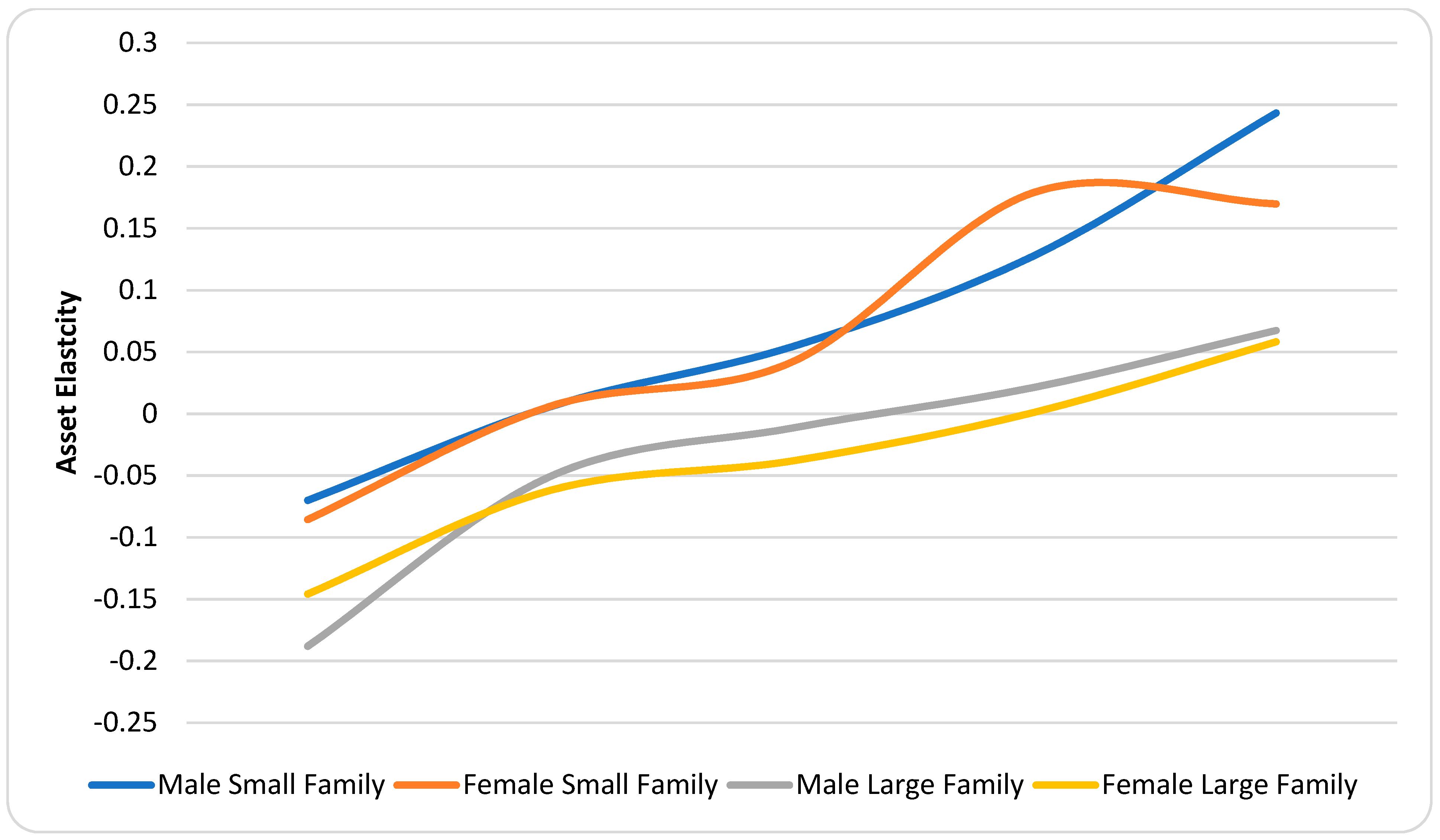
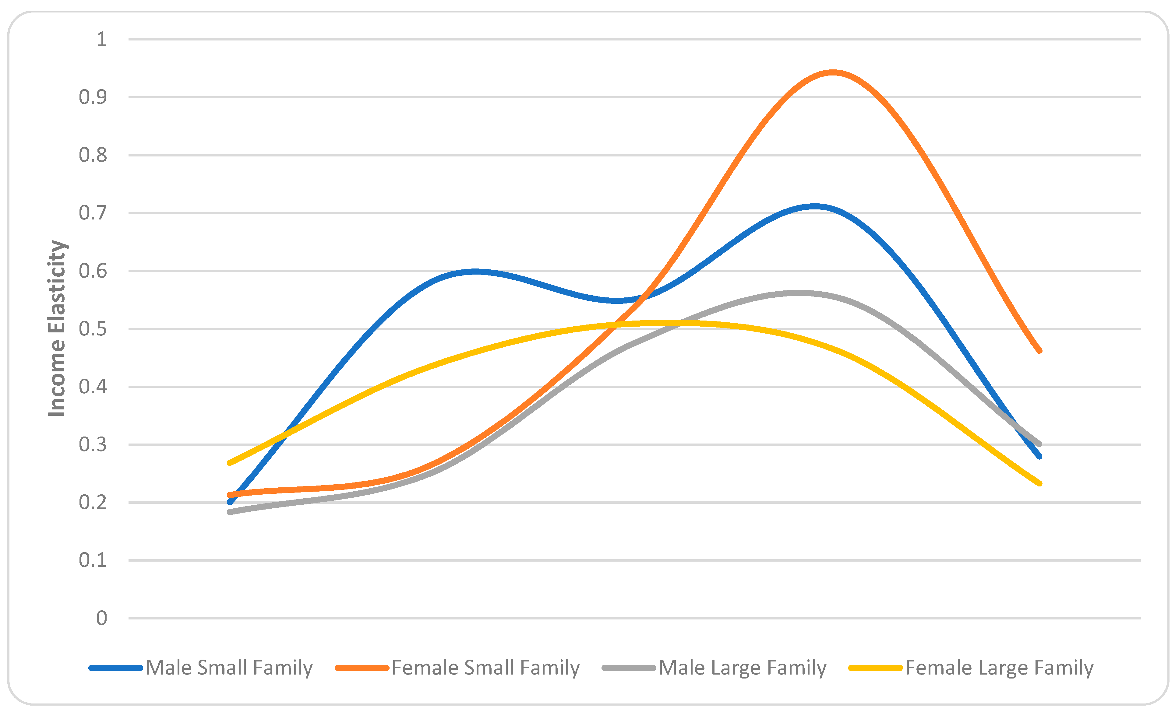
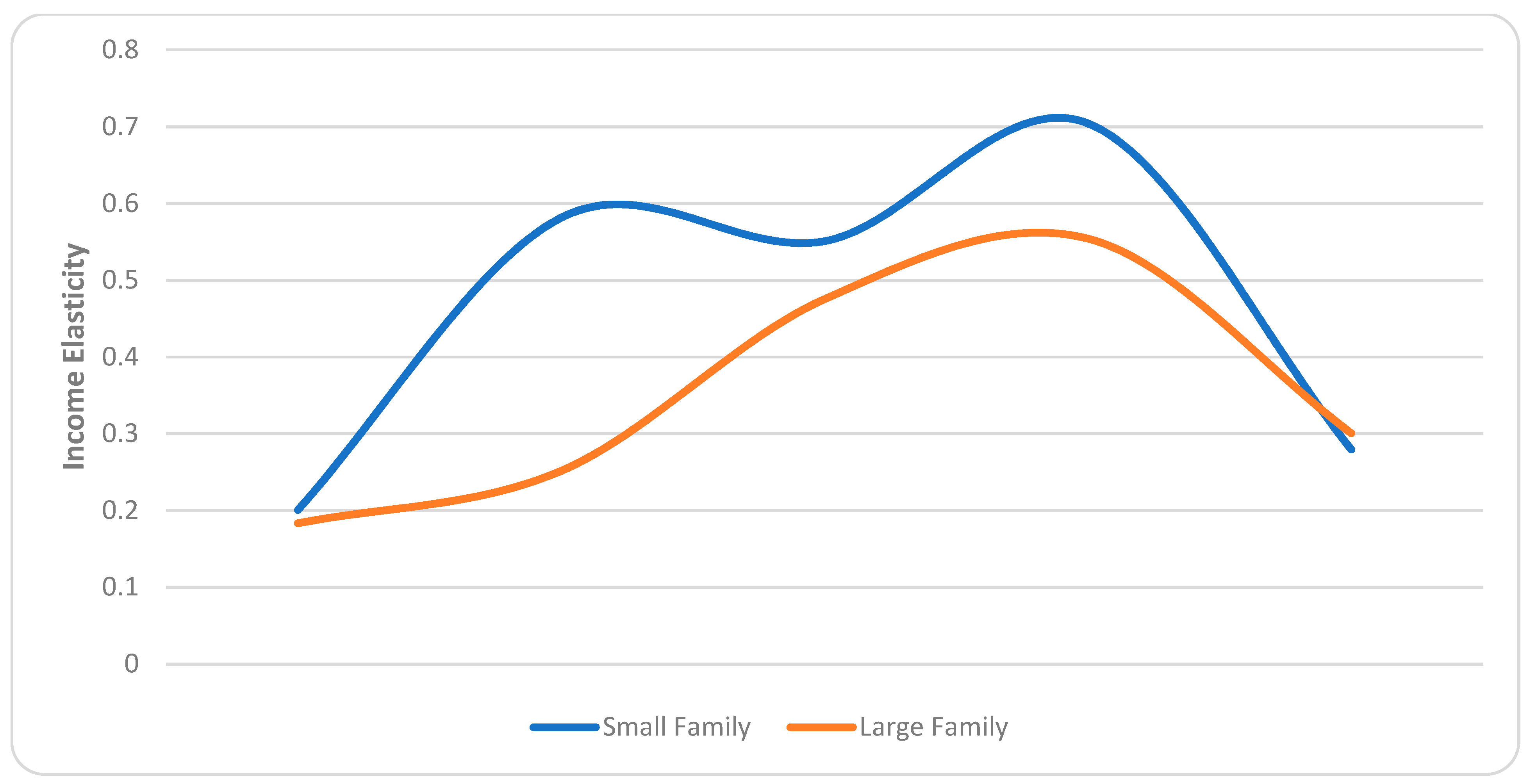
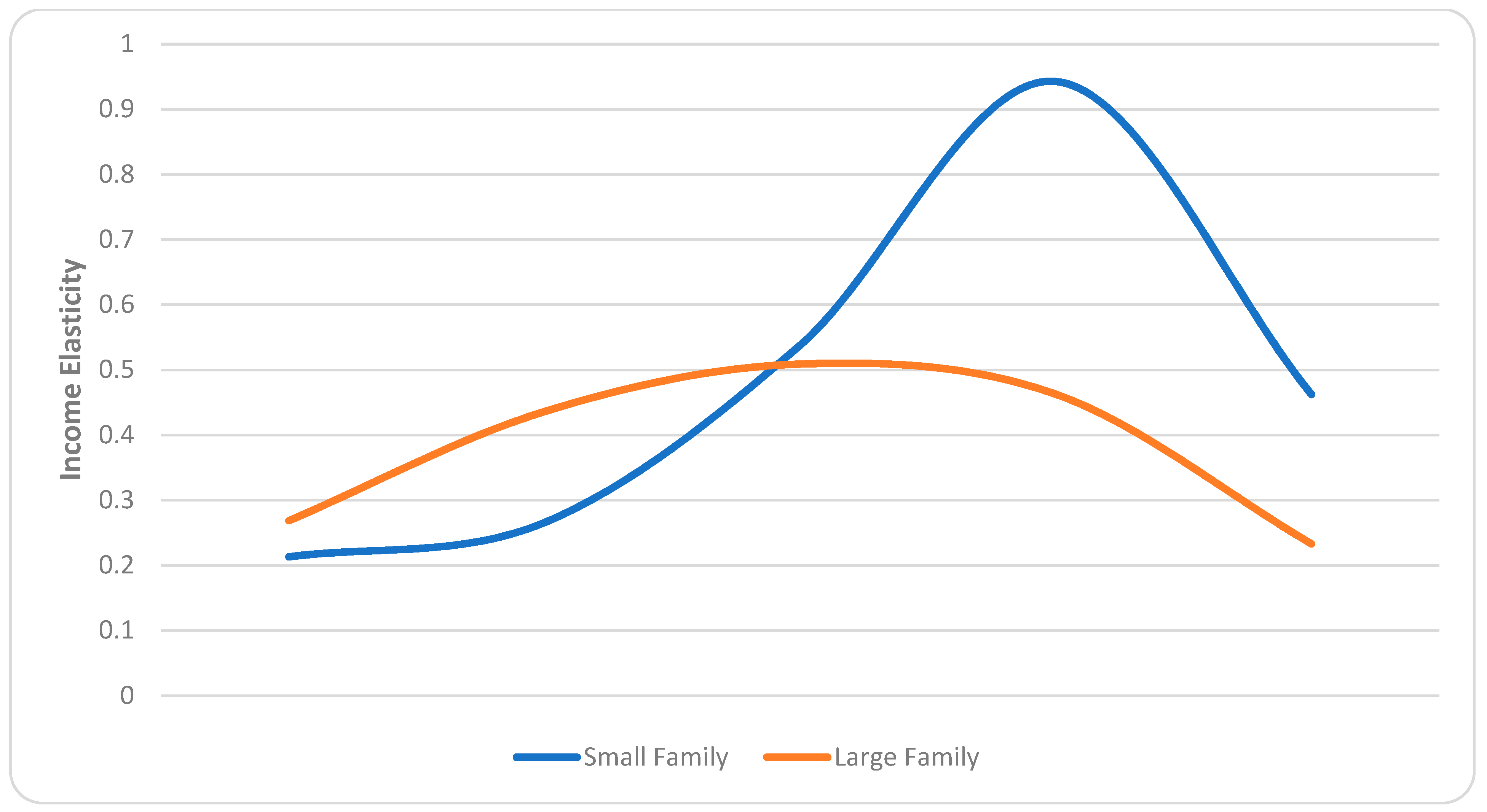
Household Income	0.20	0.21	0.18	0.27	0.58	0.27	0.25	0.44	0.55	0.54	0.48	0.51	0.70	0.94	0.55	0.46	0.28	0.46	0.30	0.23
Median Age	0.03	0.02	0.04	−0.03	0.18	0.08	0.13	−0.02	0.05	−0.08	0.05	0.07	−0.14	−0.02	0.07	0.02	0.08	−0.60	0.00	−0.03
Proximity to Death	−0.03	0.02	0.04	0.02	−0.02	0.07	−0.01	−0.13	−0.07	0.02	−0.05	−0.14	−0.16	−0.07	−0.12	−0.20	−0.09	−0.15	−0.24	−0.27
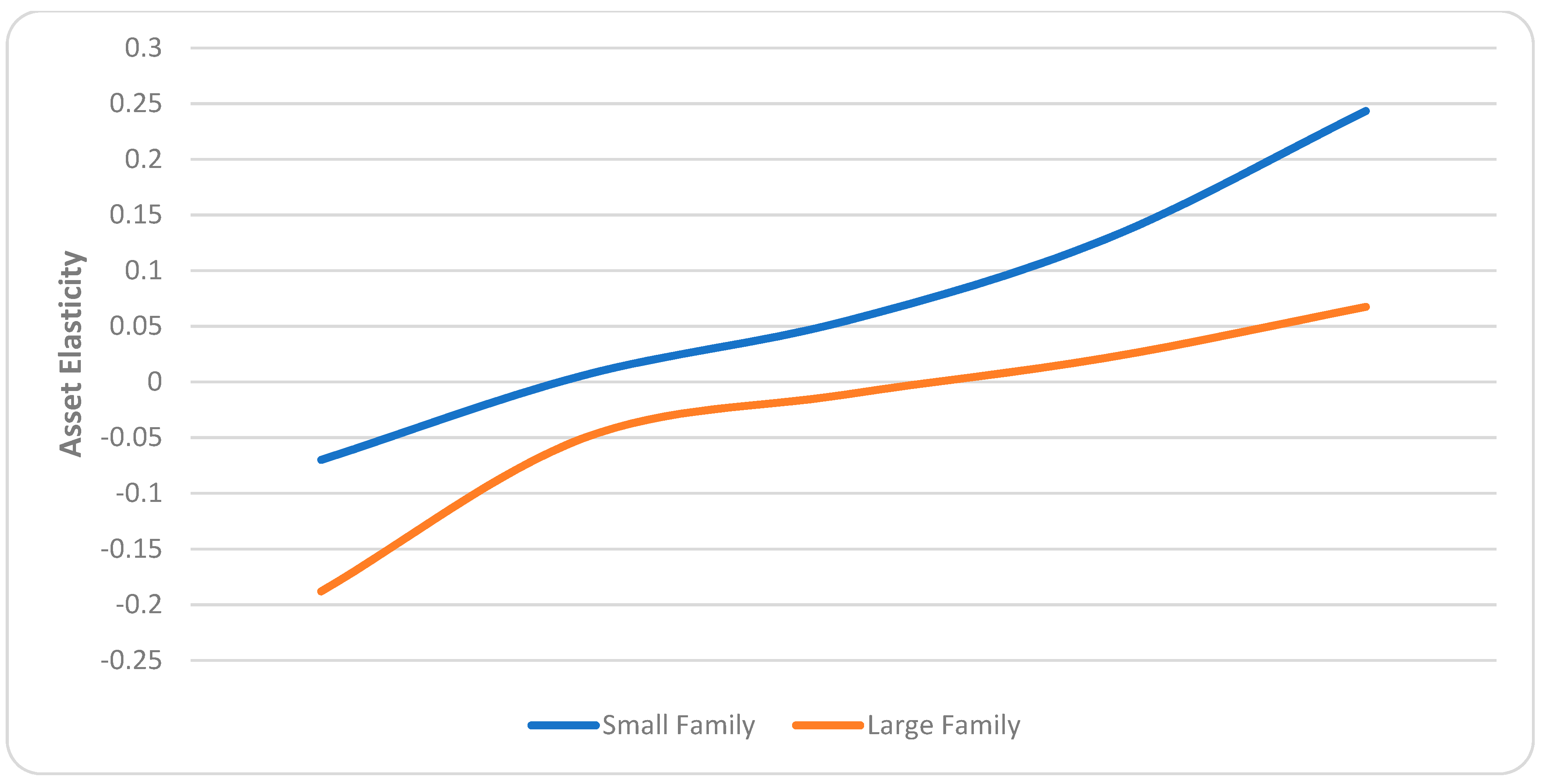
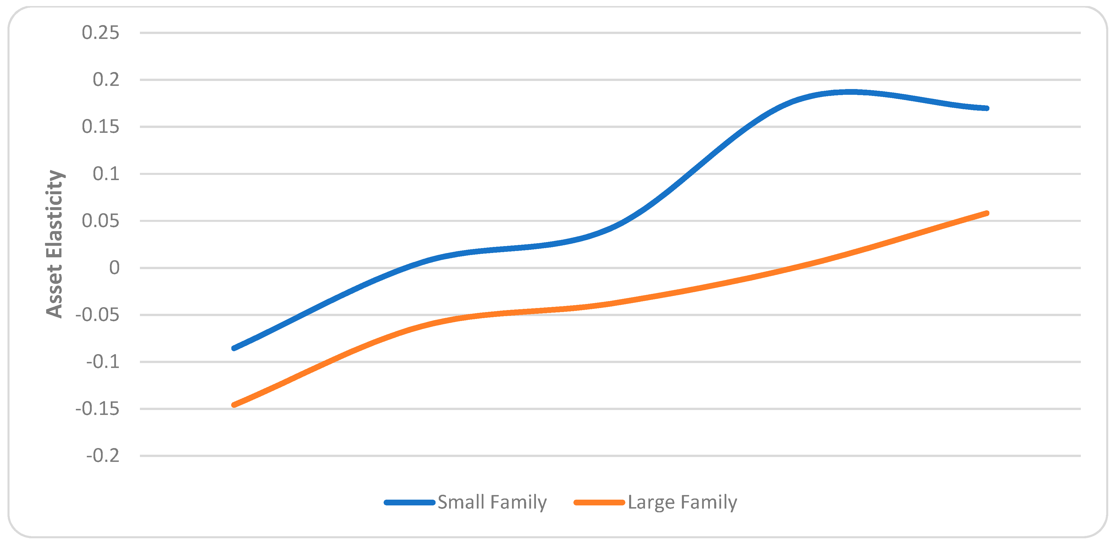
Wealth Index	−0.07	−0.09	−0.19	−0.15	0.01	0.01	−0.05	−0.06	0.05	0.04	−0.01	−0.04	0.13	0.18	0.02	0.00	0.24	0.17	0.07	0.06

and Figure 1, Figure 2, Figure 3, Figure 4, Figure 5 and Figure 6 present several insightful elasticity estimates. Foremost, while there are discernible variations in magnitudes, all income elasticities are less than unity regardless of household head gender and household size. This hints that health care behaves as a technical necessity and is consistent with the theory outlined in this paper as well as a wide range of studies based on microeconomic health datasets. Second, with the exception of female-headed large households, income elasticities in female and male headed units peaked at the 80th income quintile and then declined considerably in the highest income cohort. Third, income elasticity in male-headed small households exceeded those of their female counterparts. This is true in income quintiles 1 through 3 after which estimates for the female heads became consistently higher. Fourth, income elasticities in large mid-to-upper income households are the smallest. The pattern of income elasticity estimates in Thai households appears to be inverted U shaped in mid-to-upper income households.

Interestingly, asset elasticity estimates in small households, regardless of the head gender, is consistently higher than in larger households. This is consistent with our initial conjecture suggesting a greater likelihood of small households across income quintiles to liquidate assets to meet necessary out-of-pocket health expenses after exhausting liquid cash. Moreover, the asset elasticity of health expense is greater in male headed households.

6. Conclusions

There are implications of our study findings. Foremost, male and female household heads have different preferences that influence decisions on resource allocation for health care. This result is consistent with Alam and Mahal (2014) findings from a survey of the literature on health expenditures in low and middle-income countries. This is further reflected in the coefficient and elasticity estimates of the health expenditure model differing for male and female headed households. Our findings suggest that public policies targeting increased household healthcare consumption, and therefore improved health status, should design separate programs and incentives for male compared with female headed households in the developing countries where OOP health spending accounts for a high percentage of income share.

The empirical model results validate the hypothesis that differences in probabilities of participation in purchased healthcare differs for the different household health types. That participation probability is significantly different between genders implies that preferences are significantly different. This finding is particularly important because it motivates separate health expenditure models by household head gender. Related studies found that policies targeting micro-entrepreneurial loan and credit activities for women tend to result in women allocating more resources under their control to health care and education even in households with husbands present (Doss 2013). Mexico’s conditional cash transfer program, conditional on receipt of health care and nutritional supplements, and participation in health education sessions, are also found to be associated with improved quality of prenatal care for low-income, rural women (Barber and Gertler 2009). Well-targeted user fee exemption scheme in rural Cambodia has been deemed pro-poor in hard economic times (Flores et al. 2013). Mutual health membership organizations (MHOs) in Senegal, W. Africa, widened health care access by reducing OOP payments for hospitalization. Our study suggests that these types of programs impact women and the poor differently.

Moreover, assets as an important adjuvant to current income suggests the creation of opportunities for women to accumulate assets over which they can exercise decision control in hard economic times. This could help to sustain or prevent catastrophic declines in OOP health care spending when current incomes decline precipitously. Consequently, the health capital accumulation resulting from higher levels of health expenditures could lead to improved population health status and should spur sustainable economic development and growth (Gong et al. 2012).

One limitation of our analysis is the lack of detailed list of diseases that generates healthcare expenditure. Such a list could have provided us with detailed healthcare expenditure across different diseases by gender. Another limitation is limited access to different type of health insurance packages. Although a national database was used in the analysis, our main focus on the gender-based healthcare expenditure resulted in having a sample of household without taking into consideration of types of health insurance for analysis. Nonetheless, results from the subgroup analyses reported are robust and informative.

In summary, controlling for gender-based preference heterogeneity is important for improving the specification and estimation of healthcare demand models. Our empirical analysis of the data reconfirms the importance of variations in preferences by gender, income level and family size. More importantly, this study argues for the particularly important case of gender-specific preferences. Rather than using a dummy variable to control for household head gender, future studies of healthcare consumption should model the data separately to avoid econometric issues of endogeneity- existence of correlation between variable of interest and the error term; and selectivity bias. Finally, the findings suggest that more effective public policies should consider gender-based preference differences in the household budget allocations for disaggregated expenditures groups (healthcare, education, housing, clothing, food and recreation).

References

- Alam, Khurshid, and Ajay Mahal. 2014. Economic impacts of health shocks on households in low and middle income countries: A review of the literature. Globalization and health 10: 1–18. [Google Scholar] [CrossRef] [PubMed] [Green Version]
- Aregbeshola, Bolaji Samson, and Samina Mohsin Khan. 2018. Determinants of catastrophic health expenditure in Nigeria. The European Journal of Health Economics 19: 521–32. [Google Scholar] [CrossRef]
- Arthur, Eric, and Hassan E. Oaikhenan. 2017. The effects of health expenditure on health outcomes in Sub-Saharan Africa (SSA). African Development Review 29: 524–36. [Google Scholar] [CrossRef]
- Barber, Sarah. L., and Paul J. Gertler. 2009. Empowering women to obtain high quality care: Evidence from an evaluation of Mexico’s conditional cash transfer programme. Health Policy and Planning 24: 18–25. [Google Scholar] [CrossRef] [PubMed] [Green Version]
- Çelen, Boğaçhan, Andrew Schotter, and Mariana Blanco. 2017. On blame and reciprocity: Theory and experiments. Journal of Economic Theory 169: 62–92. [Google Scholar] [CrossRef]
- Cheung, Diana, and Ysaline Padieu. 2015. Heterogeneity of the effects of health insurance on household savings: Evidence from rural China. World Development 66: 84–103. [Google Scholar] [CrossRef] [Green Version]
- Chi, Peter. S. K., and Ping-Lung Hsin. 1999. Medical utilization and health expenditure of the elderly in Taiwan. Journal of Family and Economic Issues 20: 251–70. [Google Scholar] [CrossRef]
- Chiappori, Pierre-Andre, Amit Gandhi, Bernard Salanié, and Francois Salanié. 2009. Identifying preferences under risk from discrete choices. American Economic Review 99: 356–62. [Google Scholar] [CrossRef] [Green Version]
- Croson, Rachel, and Uri Gneezy. 2009. Gender differences in preferences. Journal of Economic Literature 47: 448–74. [Google Scholar] [CrossRef] [Green Version]
- Deaton, Angus. S., and Christina. H. Paxson. 1998. Aging and inequality in income and health. The American Economic Review 88: 248–53. [Google Scholar]
- Di Matteo, Livio. 2005. The macro determinants of health expenditure in the United States and Canada: Assessing the impact of income, age distribution and time. Health Policy 71: 23–42. [Google Scholar] [CrossRef] [PubMed]
- Dittrich, Marcus, and Kristina Leipold. 2014. Gender differences in time preferences. Economics Letters 122: 413–5. [Google Scholar] [CrossRef]
- Doepke, Matthias, and Michèle Tertilt. 2009. Women’s Liberation: What’s in it for Men? The Quarterly Journal of Economics 124: 1541–91. [Google Scholar] [CrossRef] [Green Version]
- Dohmen, Thomas, and Armin Falk. 2011. Performance pay and multidimensional sorting: Productivity, preferences, and gender. American Economic Review 101: 556–90. [Google Scholar] [CrossRef] [Green Version]
- Doss, Cheryl. 2013. Intrahousehold bargaining and resource allocation in developing countries. The World Bank Research Observer 28: 52–78. [Google Scholar] [CrossRef] [Green Version]
- Duflo, Esther. 2012. Women empowerment and economic development. Journal of Economic Literature 50: 1051–79. [Google Scholar] [CrossRef]
- Dunn, Abe. 2016. Health insurance and the demand for medical care: Instrumental variable estimates using health insurer claims data. Journal of Health Economics 48: 74–88. [Google Scholar] [CrossRef]
- Ecob, Russell, and George Davey Smith. 1999. Income and health: What is the nature of the relationship? Social Science & Medicine 48: 693–705. [Google Scholar]
- Engström, Per, and Johannes Hagen. 2017. Income underreporting among the self-employed: A permanent income approach. European Economic Review 92: 92–109. [Google Scholar] [CrossRef] [Green Version]
- Flatø, Martin, Raya Muttarak, and André Pelser. 2017. Women, weather, and woes: The triangular dynamics of female-headed households, economic vulnerability, and climate variability in South Africa. World Development 90: 41–62. [Google Scholar]
- Flores, Gabriela, Por Ir, Chean R. Men, Owen O’Donnell, and Eddy Van Doorslaer. 2013. Financial protection of patients through compensation of providers: The impact of Health Equity Funds in Cambodia. Journal of Health Economics 32: 1180–93. [Google Scholar] [CrossRef] [Green Version]
- Flory, Jeffrey A., Uri Gneezy, Kenneth L. Leonard, and John A. List. 2018. Gender, age, and competition: A disappearing gap? Journal of Economic Behavior & Organization 150: 256–76. [Google Scholar]
- Frijters, Paul, John P. Haisken-DeNew, and Michael A. Shields. 2005. The causal effect of income on health: Evidence from German reunification. Journal of Health Economics 24: 997–1017. [Google Scholar] [CrossRef] [PubMed]
- Galama, Titus J., and Hans Van Kippersluis. 2019. A theory of socio-economic disparities in health over the life cycle. The Economic Journal 129: 338–74. [Google Scholar] [CrossRef] [PubMed] [Green Version]
- Garin, Julio, Michael J. Pries, and Eric R. Sims. 2018. The relative importance of aggregate and sectoral shocks and the changing nature of economic fluctuations. American Economic Journal: Macroeconomics 10: 119–48. [Google Scholar] [CrossRef]
- Gong, Liutang, Hongyi Li, and Dihai Wang. 2012. Health investment, physical capital accumulation, and economic growth. China Economic Review 23: 1104–19. [Google Scholar] [CrossRef]
- Grigoli, Francesco, and Javier Kapsoli. 2018. Waste not, want not: The efficiency of health expenditure in emerging and developing economies. Review of Development Economics 22: 384–403. [Google Scholar] [CrossRef] [Green Version]
- Hadad, Sharon, Yossi Hadad, and Tzahit Simon-Tuval. 2013. Determinants of healthcare system’s efficiency in OECD countries. The European Journal of Health Economics 14: 253–65. [Google Scholar] [CrossRef] [PubMed]
- He, Haoran, and Marie Claire Villeval. 2017. Are group members less inequality averse than individual decision makers? Journal of Economic Behavior & Organization 138: 111–24. [Google Scholar]
- Howdon, Daniel, and Nigel Rice. 2018. Health care expenditures, age, proximity to death and morbidity: Implications for an ageing population. Journal of Health Economics 57: 60–74. [Google Scholar] [CrossRef] [PubMed] [Green Version]
- Jakovljevic, Mihajlo, Elena Potapchik, Larisa Popovich, Debasis Barik, and Thomas E. Getzen. 2017. Evolving health expenditure landscape of the BRICS nations and projections to 2025. Health Economics 26: 844–52. [Google Scholar] [CrossRef] [PubMed]
- Joshi Rajkarnikar, Pratistha, and Smita Ramnarain. 2020. Female Headship and Women’s Work in Nepal. Feminist Economics 26: 126–59. [Google Scholar] [CrossRef]
- Klasen, Stephan, Tobias Lechtenfeld, and Felix Povel. 2015. A feminization of vulnerability? Female headship, poverty, and vulnerability in Thailand and Vietnam. World Development 71: 36–53. [Google Scholar] [CrossRef]
- Lago-Peñas, Santiago, David Cantarero-Prieto, and Carla Blázquez-Fernández. 2013. On the relationship between GDP and health care expenditure: A new look. Economic Modelling 32: 124–9. [Google Scholar] [CrossRef]
- Liu, Chia, Albert Esteve, and Rocío Treviño. 2017. Female-headed households and living conditions in Latin America. World Development 90: 311–28. [Google Scholar] [CrossRef] [Green Version]
- Marmot, Michael. 2002. The influence of income on health: Views of an epidemiologist. Health affairs 21: 31–46. [Google Scholar] [CrossRef] [PubMed]
- Moore, Joel D., and John A. Donaldson. 2016. Human-scale economics: Economic growth and poverty reduction in Northeastern Thailand. World Development 85: 1–15. [Google Scholar] [CrossRef]
- Murthy, Vasudeva N. R., and Albert A. Okunade. 2016. Determinants of US health expenditure: Evidence from autoregressive distributed lag (ARDL) approach to cointegration. Economic Modelling 59: 67–73. [Google Scholar] [CrossRef]
- Okunade, Albert A., Chutima Suraratdecha, and David A. Benson. 2010. Determinants of Thailand household healthcare expenditure: The relevance of permanent resources and other correlates. Health Economics 19: 365–76. [Google Scholar] [CrossRef]
- Okunade, Albert A., Xiaohui You, and Kayhan Koleyni. 2018. Cross-country medical expenditure modeling using OECD panel data and ARDL approach: Investigating GDP, technology, and aging effects. In Health Econometrics. Bingley: Emerald Publishing Limited. [Google Scholar]
- Onah, Michael Nnachebe, and Susan Horton. 2018. Male-female differences in households’ resource allocation and decision to seek healthcare in south-eastern Nigeria: Results from a mixed methods study. Social Science & Medicine 204: 84–91. [Google Scholar]
- Pistaferri, Luigi. 2001. Superior information, income shocks, and the permanent income hypothesis. Review of Economics and Statistics 83: 465–76. [Google Scholar] [CrossRef]
- Rieger, Matthias, Natascha Wagner, and Arjun S. Bedi. 2017. Universal health coverage at the macro level: Synthetic control evidence from Thailand. Social Science & Medicine 172: 46–55. [Google Scholar]
- Said, Farah, Mahmud Mahmud, Giovanna D’Adda, and Azam Chaudhry. 2020. It is not power, but how you use it: Experimental evidence on altruism from households in Pakistan. Applied Economics Letters 27: 426–31. [Google Scholar] [CrossRef]
- Schünemann, Johannes, Holger Strulik, and Timo Trimborn. 2017. The gender gap in mortality: How much is explained by behavior? Journal of Health Economics 54: 79–90. [Google Scholar] [CrossRef] [PubMed] [Green Version]
- Subramanian, S. V., and Ichiro Kawachi. 2006. Being well and doing well: On the importance of income for health. International Journal of Social Welfare 15: S13–S22. [Google Scholar] [CrossRef]
- Swope, Kurtis J., John Cadigan, Pamela M. Schmitt, and Robert Shupp. 2008. Personality preferences in laboratory economics experiments. The Journal of Socio-Economics 37: 998–1009. [Google Scholar] [CrossRef]
- Terza, Joseph. V., Anirban Basu, and Paul J. Rathouz. 2008. Two-stage residual inclusion estimation: Addressing endogeneity in health econometric modeling. Journal of Health Economics 27: 531–43. [Google Scholar] [CrossRef] [PubMed] [Green Version]
- Van Doorslaer, Eddy, Owen O’Donnell, Ravindra P. Rannan-Eliya, Aparnaa Somanathan, Shiva Raj Adhikari, Charu C. Garg, Deni Harbianto, Alejandro N. Herrin, Mohammed Nazmul Huq, Shamsia Ibragimova, and et al. 2007. Catastrophic payments for health care in Asia. Health Economics 16: 1159–84. [Google Scholar] [CrossRef] [PubMed]
- Wiswall, Matthew, and Basit Zafar. 2018. Preference for the workplace, investment in human capital, and gender. The Quarterly Journal of Economics 133: 457–507. [Google Scholar] [CrossRef] [PubMed]
- Xu, Ke, David B. Evans, Guido Carrin, Ana Mylena Aguilar-Rivera, Philip Musgrove, and Timothy Evans. 2007. Protecting households from catastrophic health spending. Health Affairs 26: 972–83. [Google Scholar] [CrossRef] [Green Version]