Individualization in Online Markets: A Generalized Model of Price Discrimination through Learning

Abstract

This paper builds a theoretical framework to model individualization in online markets. In a market with consumers of varying levels of demand, a seller offers multiple product bundles and prices. Relative to brick-and-mortar stores, an online seller can use pricing algorithms that can observe a buyer’s online behavior and infer a buyer’s type. I build a generalized model of price discrimination with Bayesian learning where a seller offers different bundles of the product that are sized and priced contingent on the posterior probability that the consumer is of a given type. Bayesian learning allows the seller to individualize product menus over time as new information becomes available. I explain how this strategy differs from first- or second-degree price discrimination models and how Bayesian learning over time affects equilibrium values and welfare.

1. Introduction

In the first quarter of the year 2023, online retail spending accounted for about 15% of the total retail spending in the US [1]. The convenience of online shopping, as well as the health concerns associated with in-store shopping during the pandemic, were major factors in the expansion of online markets. This is happening at a time when the technology of communication, tracking, data collection and processing is developing at a fast pace.

The increased access to information in online markets has affected market participants in profound ways. For example, the availability of consumer reviews for products has increased consumer confidence as they are better able to identify credible sellers, which in turn has increased sales [2,3,4,5]. On the other hand, sellers have utilized buyers’ information that is available online to individualize products and prices. Many online sellers have used pricing algorithms, which are computer programs that can use the available high-frequency information regarding buyers’ behavior, market demand, cost and competition to more accurately determine and adjust prices and quantities.

Such technological developments spurred research investigating firm behavior in online markets and how it differs from the well-understood behavior of brick-and-mortar stores. Some research has focused on the potential for pricing algorithms used by competing firms to collude as they learn that collusion results in higher profit [6,7,8,9]. However, other research has focused on the enhanced ability of firms to price discriminate based on the increased availability of consumer information. Sellers can access buyers’ information, e.g., age, gender and location. In addition, sellers may track buyers’ behavior online by identifying websites they have visited and their past purchases. (There is anecdotal evidence that sellers use buyers’ demographic and geolocation information to generate the products displayed to a user as well as to set their prices. It was reported that Staples.com charged buyers different prices based on their location. Buyers who were in close proximity to an Office Depot or Office Max were charged lower prices for the same products than buyers who had less access to competing stores [10]. Other retailers, for example, Home Depot, were also found to alter prices based on the location of the user [11]. In 2000, Amazon charged people different prices for the same DVD. This was discovered by a buyer who erased the cookies on his device and saw the price drop [12]. Similarly, online travel agencies have relied on cookies and more advanced technologies to identify when buyers are most ready to buy [13]. Several researchers have tried to find evidence of price discrimination in online markets. They have also tried to identify the factors on which price discrimination is based (e.g., demographic variables, location or click history) [14,15,16,17,18,19].

However, the theoretical contributions to this topic are very limited. In fact, the theoretical research on online markets has utilized very simplified economic models that do not capture the realities of online markets. By relying on the existing price discrimination theories (first- and second-degree) to model online firm behavior, these models represent extreme outcomes where either (1) the firm can identify each buyer’s type with certainty (and thus they adopt a first-degree price discrimination model) or (2) the firm cannot identify a buyer’s type but knows the distribution of buyer types in the market (and thus use a second- or third-degree price discrimination model). For example, Acquisiti and Varian [20] use a second-degree pricing model, where firms discriminate based on consumers’ purchase histories. Bang and Kim [21] use a second-degree price discrimination model, where the firm chooses where to sell (online, offline or both) and chooses the level of product information to provide to each market. Prasad et al. [22] use a second-degree price discrimination model to analyze product bundling online with myopic and strategic buyers. Alternatively, other research papers have relied on first-degree price discrimination models to describe online behavior. For example, Rayna et al. [23] use a first-degree price discrimination model to illustrate the potential to achieve a win–win scenario for firms and buyers in online markets when buyers have an incentive to misrepresent their types. Also, Shiller [24] shows that using data for a Netflix subscription that improves access to buyers’ information leads to significantly higher profits. He thus concludes that personalization (synonymous with first-degree price discrimination) is likely to become the norm in markets. He argues that first-degree price discrimination, which used to be just a theoretical illustration, will become the modelling approach for firm behavior.

I argue that neither first nor second-degree price discrimination theories adequately address firm behavior in online markets, where sellers continuously use the available information to improve their ability to predict consumer types and adjust or “individualize” quantities and prices accordingly. I develop a model of individualization in online markets that offers a generalized price discrimination framework that describes all price discrimination outcomes resulting from access to different levels of information. The firm uses the available consumer information to make inferences about the consumer’s type and accordingly offers him a menu of products with different prices and sizes. I use Bayesian learning which has been used in many contexts to model learning [25,26,27]. to model how the firm uses newly available information in every time period to update its inference about the buyer type and adjust the menu of products offered. As the firm obtains more information over time, the model results converge to those under first-degree price discrimination. However, when the firm has no access to buyers’ information, the model results become identical to those under second-degree price discrimination models. Our results indicate that individualization reduces the consumer surplus of most types of buyers and increases firm profit. Overall, social welfare improves as quantities approach their socially optimal levels.

2. The Model

Consider an online market with I consumer types that differ in the extent of demand and, therefore, their willingness to pay for the product. Let $V_{ij}$ denote the utility of a type i consumer, where I = 1 to I, who buys a bundle, j, where j = 1 to J. Consistent with the price discrimination literature, I assume $V_{ij}>V_{kj}$ and $V_{ij}^{\prime }>V_{ij}^{\prime }$ for I > k, i.e., a higher-demand buyer has a higher total and marginal utility from buying bundle j [28,29]. I assume a monopoly (the assumption of a monopoly market is widely used in the literature on price discrimination, where some monopoly power is a prerequisite for building the model. While it can potentially be a limiting assumption and should be relaxed in future research, it allows me to focus on the process of individualization and learning) firm that produces goods at a constant unit cost of c. The firm knows $V_{ij}$. The number of buyers in the market is denoted by N, and the number of type i buyers is denoted by $n_i$. The firm offers a menu of J bundles of the product, i.e., J different product sizes and prices.

2.1. The Standardized Product Menu

I start by assuming a one-period model where the firm cannot identify a buyer’s type at the point of purchase. Following the price discrimination literature, I assume the firm offers J bundles of the product, where J = I, i.e., the number of bundles offered equals the number of consumer types. (Under certain parameter values, it is possible for the firm to produce fewer bundles than the number of consumer types, i.e., J < I. In the following section, we assume parameter values that ensure the firm produces a number of bundles equal to the number of buyer types.) Each bundle has $Q_i$ units of the product and sells at a price of $R_i$. While the firm does not know with certainty the type of consumer, it assumes that he is probably type i (the prior). $p_i$ is given by $p_i=\frac{n_i}{N}$ where $\sum _{i=1}^I{p}_i=1$. Based on this information, the firm offers him a maximum of I bundles to choose from. The firm maximizes the expected profit, π, realized from selling to consumer i, given by

$$\pi ={\sum }_{i=1}^I{p}_i(R_i-c{Q}_i)$$

(1)

The firm chooses $Q_i,$ where i = 1 to I, to maximize the expected profit in (1), subject to the participation and self-selection constraints given by Equations (2) and (3), respectively, as follows:

$$V_{ii}-R_i\ge 0,$$

(2)

and

$$V_{ii}-R_i\ge V_{ij}-R_j,$$

(3)

where $V_{ij}$ denotes the utility of a consumer of type i buying bundle j. The self-selection constraint in (3) ensures that consumer i chooses the ith bundle over any other bundle. The participation constraint in (2) ensures he chooses to buy rather than to not buy. Simplifying (2) and (3), I obtain the price of bundle i:

$$R_i=V_{ii}-{\sum }_{j=2}^i(V_{j j-1}-V_{j-1 j-1})$$

(4)

for i > 1 and $R_1=V_{11}$.

Differentiating (1) with respect to $Q_i$ gives the first-order condition,$F_i$, as follows:

$$F_i=p_i\left(\frac{\mathsf{\partial }{R}_i}{\mathsf{\partial }{Q}_i}-c\right)+{\sum }_{j=i+1}^I{p}_j\left(\frac{\mathsf{\partial }{R}_j}{\mathsf{\partial }{Q}_i}\right)$$

(5)

Note that $\frac{\mathsf{\partial }{R}_i}{\mathsf{\partial }{Q}_i}=P_i$, where $P_i$ is consumer i’s inverse demand. Since $\sum _{j=i+1}^I{p}_j\left(\frac{\mathsf{\partial }{R}_j}{\mathsf{\partial }{Q}_i}\right)<0$ for all i $\ne$ I, in equilibrium (where $F_i$= 0), the firm offers $Q_i$, where $\frac{\mathsf{\partial }{R}_i}{\mathsf{\partial }{Q}_i}=V_{ii}^{\prime }=P_i>c$. Therefore, all the quantities offered (except for $Q_I$, the largest size bundle (the largest bundle offered, $Q_I$, is the one where price equals the marginal cost, $P_I=c$, since $\sum _{j=i+1}^I{p}_{jt}\left(\frac{\mathsf{\partial }{R}_j}{\mathsf{\partial }{Q}_I}\right)=0$)) are not socially optimal, i.e., are below the point where price equals marginal cost. The distortion in $Q_i$ increases as $p_{jt}$ increases, where $j\ge i+1$. Thus, as the likelihood that a buyer is of a higher demand type increases, the quantity designed for lower-demand buyers decreases. This is necessary given that the firm does not know the buyer’s type with certainty and therefore chooses the quantities to ensure self-selection. Increasing the quantity offered to lower-demand-type buyers would lead a given buyer to move away from the bundle intended for him.

The equilibrium outcome in this case is consistent with that of the second-degree price discrimination models (see, for example, Tirole [29]), where in equilibrium, the firm distorts the quantity provided to all buyers except the one offered to the highest-demand buyer to ensure incentive compatibility. In our case, the firm distorts all bundles in the menu offered to a given consumer except the largest-sized bundle. Since consumers are unidentifiable at purchase, the firm offers a standardized menu of products to all consumers.

2.2. Bayesian Learning

Alternatively, an online firm can use a pricing algorithm that tracks buyers’ online behaviors to better identify their types. I assume that while buyers differ in terms of utility, they also differ in terms of another parameter, ${\beta }_t$, where ${\beta }_t=0$ or 1. ${\beta }_t$ represents an online behavior that can be observed by the pricing algorithm at time t. ${\beta }_t$ can represent, for example, whether a buyer buys luxury products or not at time t. I assume that ${\beta }_t$ correlates with a buyer’s type such that $P\left({\beta }_t=1|i\right)$ > $P\left({\beta }_t=1|j\right)$ for i > j, i.e., ${\beta }_t$ = 1 is more likely for higher-demand-type buyers.

I model the firm’s maximization problem, assuming that the firm can observe ${\beta }_t$ for consumer i at time t = 2 to T and sets the menu prices and quantities accordingly. I assume that at time t = 1, the firm does not observe ${\beta }_1$ and, therefore, produces a standardized menu, as in the previous section. At t = 1, the firm determines the quantities offered based on the prior. I use this as a benchmark case for comparison with the individualized equilibrium outcomes in periods t = 2 to T. Every period, the firm updates the probability distribution of buyers based on ${\beta }_t$.

Following the work of Gelman et al. [30], we define $p_{it}$ to be the Bayesian probability that a buyer is of type i, conditional on the observed values of β and the prior,$p_i$. The probability in period t that a buyer is of type i is given by

$$p_{it}=p\left(i|{\beta }_1,..,{\beta }_t\right)=\frac{P\left({\beta }_1,\dots .,{\beta }_t|i\right)}{P{(\beta }_1,\dots ,{\beta }_t)}. p_i$$

(6)

Equation (6) can be modified to reflect the Bayesian updating of $p_{it}$ from the period t − 1, where

$$p_{it}=\frac{P\left({\beta }_t|i\right)}{P\left({\beta }_t\right)}. p_{it-1}$$

(7)

In that case, $p_{it-1}$ becomes the new prior, which is updated as new information becomes available in period t.

In light of the updated probability distribution, the firm chooses $Q_{it}$ to maximize the expected profit in period t, given by

$${\pi }_{\beta }^t={\sum }_{i=1}^I{p}_{it}(R_i-c{Q}_i)$$

(8)

This is subject to the participation and self-selection constraints defined in (2) and (3). The resulting menu (prices and quantities) is individualized based on consumer i’s observed values of ${\beta }_t$. Hence, the firm deviates away from offering a standardized menu to all buyers, as illustrated in Section 2.1, and offers an individualized menu. The individualized equilibrium will be described in the following section.

3. The Individualized Equilibrium under Bayesian Learning

In this section, I solve for market equilibrium and show how Bayesian learning changes the equilibrium values over time. I start by investigating how ${\beta }_t$ determines the probability distribution across types for a consumer i, which in turn affects the menu prices and quantities offered to him. I investigate the resulting effects on the equilibrium, particularly focusing on $Q_i$ and $R_i$, the incentive-compatible bundle intended for consumer i.

For simplicity, I assume three buyer types, a high-demand (H), medium-demand (M) and low-demand (L), and I assume $n_H=n_M=n_L$. I assume that in the period t = 1, the firm does not observe ${\beta }_1$ and, therefore, produces a standardized menu. At t = 1, the firm determines the quantities offered based on the prior $p_{H1}=p_{M1}=p_{L1}$ = 1/3. I use this as a benchmark for comparison with the individualized equilibrium outcomes in periods 2 to T.

However, for t > 1, the firm observes ${\beta }_t$ for a given buyer and determines the probability distribution across types of consumers, conditional on the current and all past values of ${\beta }_t$. The firm then offers an individualized menu, on which prices and quantities are set accordingly.

The Bayesian probability that a buyer is of type i (where i = H, M or L) in period t is denoted by $p_{it},$ conditional on this probability in the previous period, $p_{it-1}$, and the observed value of ${\beta }_t,$ based on Equation (7) (note that the denominator in (9), $\sum _j{p}_{jt-1}.p_{\beta j}=p_{Ht-1}.p_{\beta H}+p_{Mt-1}.p_{\beta M}+p_{Lt-1}.p_{\beta L},$ is simply the probability that ${\beta }_t$ is one, which is the denominator in (7). Similarly, the denominator in (10), $\sum _j{p}_{jt}-1.(1-p_{\beta j})$, is the probability that ${\beta }_t$ is 0), as follows:

$$p_{it}=\frac{p_{\beta i}}{\sum _j{p}_{jt-1}.p_{\beta j}} . p_{it-1} \mathrm{if} {\beta }_t =1,$$

(9)

and

$$p_{it}=\frac{(1-p_{\beta i})}{\sum _j{p}_{jt-1}.(1-p_{\beta j})}.p_{it-1} \mathrm{if} {\beta }_t =0,$$

(10)

where j = H, M or L. Thus, (9) and (10) demonstrate how the firm updates its expectations based on newly available information. For simplicity and without a loss of generality, I assume that $p_{\beta H}=P\left({\beta }_t=1|H\right)=0.9$,$p_{\beta M}=P\left({\beta }_t=1|M\right)=0.8$ and $p_{\beta L}=P\left({\beta }_t=1|L\right)=0.7$. The analysis below will first explain how the probability distribution across buyer types for a given consumer changes overtime in response to the observed value of ${\beta }_t$ (Proposition 1). Then, the analysis will show the corresponding effect on the equilibrium quantities and prices (Propositions 2–4). Proofs of the propositions are provided in Appendix A.

Proposition 1. 

The probability distribution across types at time t depends on ${\beta }_t$.

i.

If  ${\beta }_t$ = 1, then (a)  ${∆p}_{Ht}$ > 0, (b)  ${∆p}_{Mt}$ > 0 if  $p_{Lt-1}>p_{Ht-1}$ and (c)  ${∆p}_{Lt}$ < 0. 

ii.

If  ${\beta }_t$ = 0, then (a)  ${∆p}_{Ht}$ < 0, (b)  ${∆p}_M$ < 0 if  $p_{Lt-1}>p_{Ht-1}$ and (c)  ${∆p}_{Lt}$ > 0.

If ${\beta }_t$ = 1, then ${∆p}_{Ht}$ > 0 and ${∆p}_{Lt}$ < 0, i.e., it becomes more likely that the buyer is a high-demand type and less likely that he is a low-demand type in comparison to the previous period. However, the effect on ${∆p}_{Mt}$ is determined by the previous period probabilities. ${∆p}_{Mt}$ > 0 in response to ${\beta }_t$ = 1 only if $p_{Lt-1}$ > $p_{Ht-1}$.

I assume the demand functions of each group are linear in price and are given by $P_H=A_H-B_H{Q}_H$, $P_M=A_M-B_M{Q}_M$ and $P_L=A_L-B_L{Q}_L$, and the unit cost is constant and given by c, where $A_H$ > $A_M$ > $A_L$ > c. I also assume $\frac{A_H}{B_H}>\frac{A_M}{B_M}>\frac{A_L}{B_L}$ to ensure the demand functions do not intersect. Based on those functions, the equilibrium quantities offered to consumer i are given by the following (the equilibrium quantities are obtained by maximizing the profit, as shown in (7), where the bundle prices, $R_i$, are given in (A9)–(A11)):

$$Q_{Ht}=\frac{A_H-c}{B_H}$$

(11)

$$Q_{Mt}=\frac{A_M\left(p_{Mt}+p_{Ht}\right)-A_H{p}_{Ht}-c{p}_{Mt}}{B_M\left(p_{Mt}+p_{Ht}\right)-B_H{p}_{Ht}}$$

(12)

$$Q_{Lt}=\frac{A_L-A_M\left(1-p_{Lt}\right)-\mathrm{c}\left(p_{Lt}\right)}{{B_L-B}_M(1-p_{Lt})}$$

(13)

where $p_{Ht}, p_{Mt}$, $p_{Lt}$ are the probabilities that consumer i is a high-demand, medium-demand or low-demand type. Note that the output levels, except $Q_{Ht}$, depend on the probability distribution across the types. (Note that if $p_{Lt}$< $\frac{A_M-A_L}{A_M-c}$, then $Q_{Lt}<0$, and in that case, we set $Q_{Lt}=0$. Thus, when the likelihood that the buyer is of a low-demand type is low enough, the firm does not offer a low bundle. Similarly, when $p_{Mt}$ < $\frac{A_H-A_M}{A_M-c}{p}_{Ht}$, the firm does not offer a medium-sized bundle).

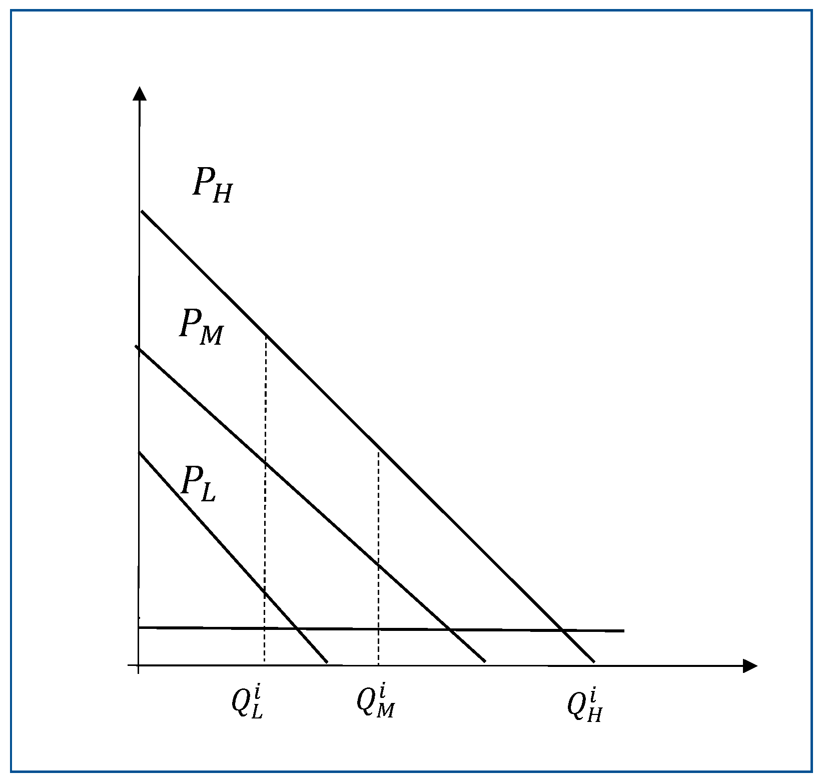
The equilibrium quantities and prices are illustrated in Figure 1. Figure 1 shows that $Q_{Ht}$ is set where $P_H$ equals the marginal cost. However, $Q_{Mt}$ and $Q_{Lt}$ are below the point where the price equals the marginal cost. The under provision of the output is consistent with the results from the second-degree price discrimination theory, as explained in Section 2.1. This is necessary to ensure self-selection, i.e., to ensure that the high-demand (or medium-demand)-type buyer does not buy the medium (or low) bundle.

The change in the output levels over a single period of time will depend on ${\beta }_t,$ as follows.

Proposition 2. 

The menu quantities offered to consumer i change as follows:

i.

If  ${\beta }_t=1$, then  $\frac{\mathsf{\Delta }{Q}_{Lt}}{\mathsf{\Delta }t}$ < 0. 

ii.

If  ${\beta }_t=0$, then  $\frac{\mathsf{\Delta }{Q}_{Lt}}{\mathsf{\Delta }t}$ > 0. 

iii.

$\frac{\mathsf{\Delta }{Q}_{Mt}}{\mathsf{\Delta }t}$ will depend on the parameter values in either case.

The firm adjusts the menu quantities (except $Q_{Ht}$) in response to the change in the probability distribution across the types of consumers while ensuring self-selection. From proposition 1, when ${\beta }_t=1$, it becomes more likely that consumer i is a high-demand-type consumer, $\mathsf{\Delta }{p}_{Ht}$ > 0, and less likely that he is a low-demand-type consumer, $\mathsf{\Delta }{p}_{Lt}$ < 0. This, in turn, will result in a decrease in $Q_{Lt}$ and a decrease in $Q_{Mt}$ only if $\mathsf{\Delta }{p}_{Mt}$ < 0. The firm can adjust quantities to reduce the information rent given to consumer i and thus raise profit while still ensuring incentive compatibility.

The menu prices will change over a single period of time in response to the changes in menu quantities, as described in Proposition 3.

Proposition 3. 

The menu prices offered to consumer i will change as follows:

i.

If ${\beta }_t=1$, then $\frac{\mathsf{\Delta }{R}_{Lt}}{\mathsf{\Delta }t}$ < 0.

ii.

If ${\beta }_t=0$, then $\frac{\mathsf{\Delta }{R}_{Lt}}{\mathsf{\Delta }t}$ > 0.

iii.

$\frac{\mathsf{\Delta }{R}_{Ht}}{\mathsf{\Delta }t}$ and $\frac{\mathsf{\Delta }{R}_{Ht}}{\mathsf{\Delta }t}$ will depend on the relative parameter values.

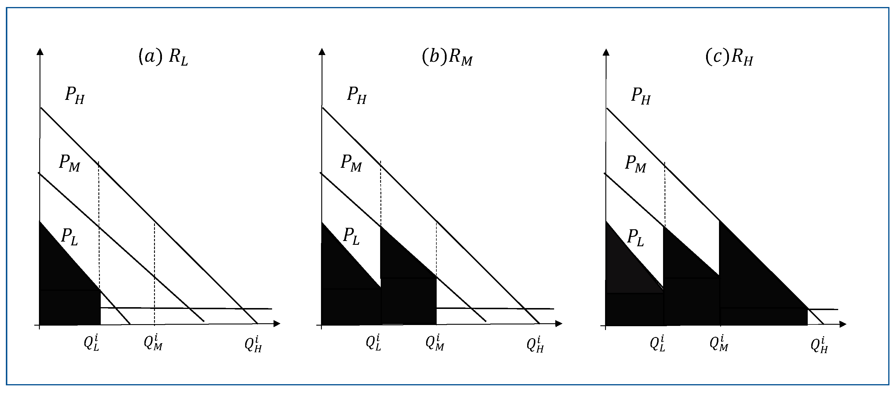
If ${\beta }_t=1$, then $Q_{Lt}$ decreases, as is clear from Proposition 2, and, in turn, $R_{Lt}$ also decreases. The shaded areas in Figure 2 show the menu prices of each of the three bundles. It is clear from Figure 2a that a reduction in $Q_{Lt}$ reduces $R_{Lt}$. If everything else is equal, this change will increase $R_{Mt}$, as shown in Figure 2b, as $Q_{Lt}$ moves to the left. The net effect on $R_{Mt}$ will depend on how $Q_{Mt}$ responds to ${\beta }_t=1$. If $∆Q_{Mt}$ > 0, then $R_{Mt}$ increases. Similarly, the change in $R_{Ht}$ will depend on how $Q_{Mt}$ and $Q_{Lt}$ change. If $∆Q_{Mt}$ > 0 in response to ${\beta }_t=1$, then the change in $R_{Ht}$ is ambiguous. Based on Figure 2c, the effect of $∆Q_{Mt}$ > 0 while $∆Q_{Lt}$ < 0 will depend on the relative sizes of the changes as well as the demand curves.

The above analysis explains how the menu prices and quantities change from one period to another in response to the observed value of ${\beta }_t$. While some of these changes from one period to another may be ambiguous, the equilibrium prices and quantities for a given buyer type will converge to certain values. I explain this in Proposition 4 below, which explains how the prices and quantities of the incentive-compatible bundle converge over time.

Proposition 4. 

The equilibrium prices and quantities of the incentive-compatible bundle will converge as follows:

i.

$Q_{it}^{}$ → $\frac{A_i-c}{B_i}$ for consumer i, for i = M and L;

ii.

$R_{it}\to {\int }_0^{Q_{it}}{P}_i$ for consumer i, where i = H, M and L.

Bayes theorem and the law of large numbers imply that through learning, $p_{it}^{}$→1 for consumer i, and $p_{jt}^{}$→0 for j ≠ I [30]. As a result, the quantity of the incentive-compatible bundle will increase over time to the point where demand meets the marginal cost (except for the quantity of the high bundle, which does not change). As a result, the price of the incentive-compatible bundle will increase. For the high-demand buyers and medium-demand buyers, that increase eliminates the consumer surplus, which is extracted by firms (the consumer surplus of the low-demand buyer is always zero). Thus, individualization over time eliminates the consumer surplus, which becomes producer profit, an outcome that is equivalent to the equilibrium under the first-degree price discrimination models.

4. Simulation

In this section, I simulate market equilibrium, where the firm learns over time and individualizes its menu of products for a given buyer. In this section, I generate values for ${\beta }_t$ and show how the firm responds to the newly available information in period t by changing prices and quantities. I assume an equal number of buyers in each group, i.e., in the period t = 1, the priors are $p_{H1}=p_{M1}=$ $p_{L1}=$ 1/3. I assume the firm observes ${\beta }_t$ for a given buyer for t = 2 to 21. I generate values of ${\beta }_t$ (0 or 1) for each buyer type for 20 periods such that $p_{\beta H}=P\left({\beta }_t=1|H\right)=0.9$,$p_{\beta M}=P\left({\beta }_t=1|M\right)=0.8$ and $p_{\beta L}=P\left({\beta }_t=1|L\right)=0.7$, as assumed in Section 3. After generating values for ${\beta }_t$, the probability distribution of each buyer type is calculated in each of the 20 periods using Equations (9) and (10).

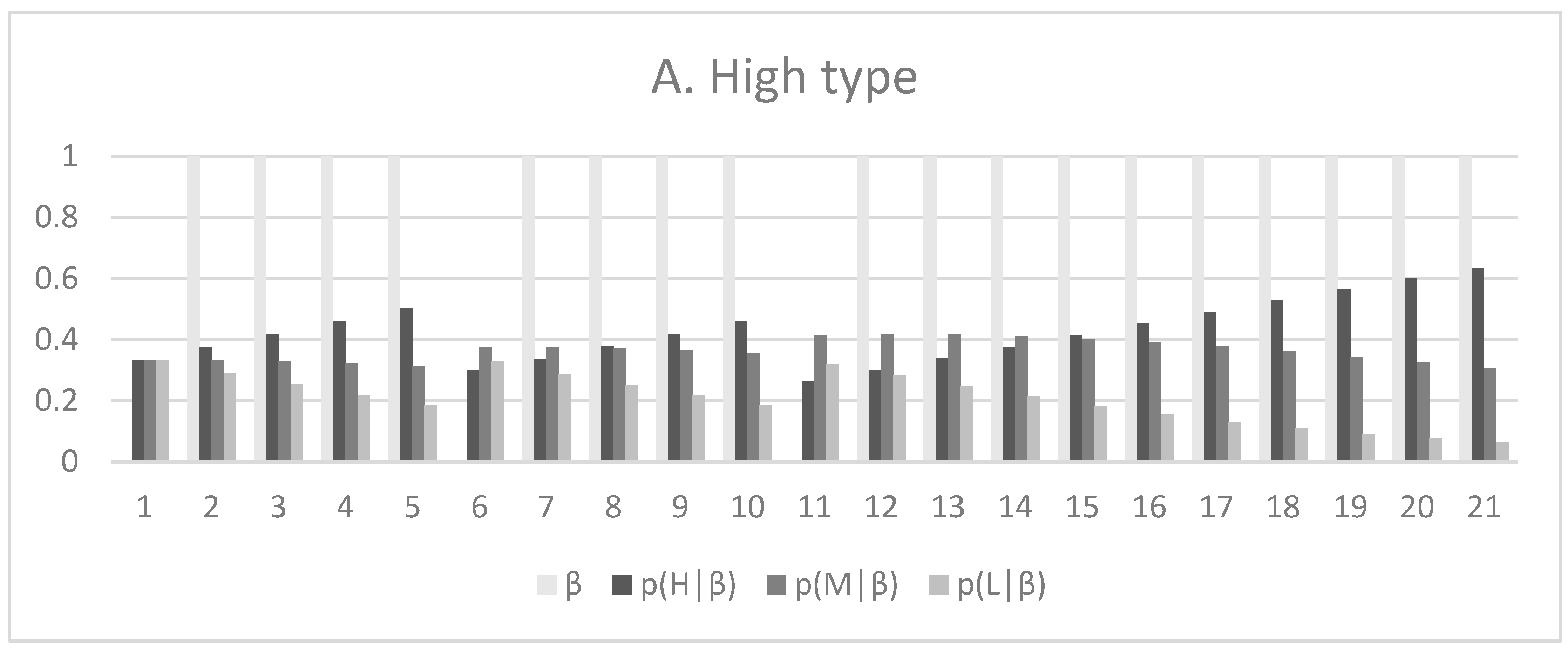
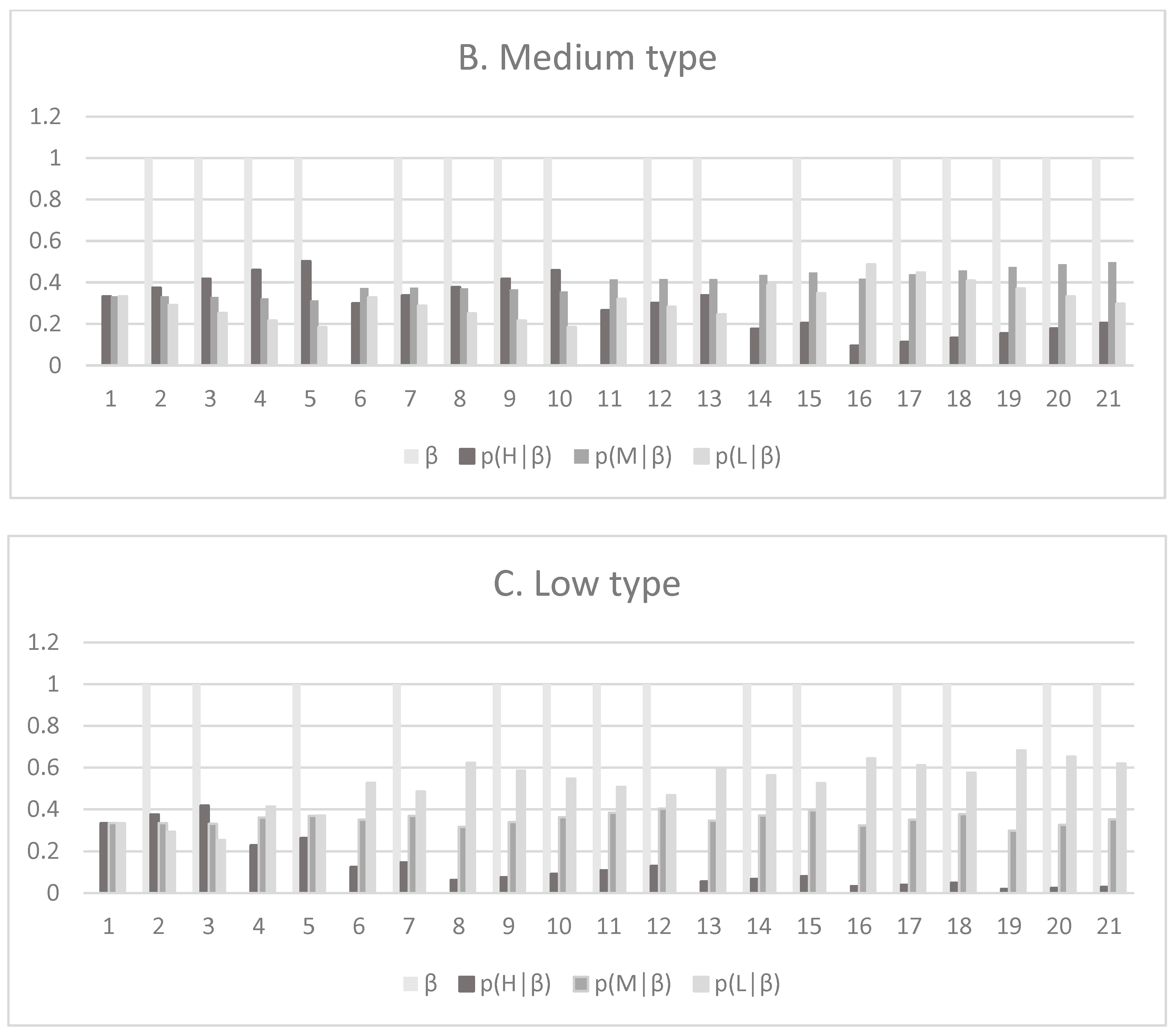
Figure 3 shows ${\beta }_t$ for the different buyer types, (represented by the light gray bars) and the resulting probability distributions. As stated in Proposition 1,$P\left(H|\beta \right)$ decreases and $P\left(L|\beta \right)$ increases in response to ${\beta }_t$ = 0, which suggests that the buyer is less likely to be a high-demand-type consumer and more likely to be a low-demand-type consumer, and vice versa. In periods where ${\mathit{p}}_{\mathit{L}\mathit{t}-1}<{\mathit{p}}_{\mathit{H}\mathit{t}-1}$, ${\mathit{p}}_{\mathit{M}\mathit{t}}$ increases (for example, Figure 3A, t = 5 to 6). Figure 3A represents a high-demand-type buyer, where $P({\beta }_t=1)=0.9$. Thus, I assume ${\beta }_t$ = 1 in 18 out of 20 periods, i.e., for all t except two periods, specifically t = 6 and t = 11, where ${\beta }_t$ = 0. Figure 3B represents a medium-demand-type buyer (${\beta }_t$ = 1 in 16 out of 20 periods), while Figure 3C shows a low-demand-type buyer (${\beta }_t$ = 1 in 14 out of 20 periods). Note that through Bayesian learning, the firm moves closer to identifying the buyer type. For example, at t = 21 in Figure 3A, while the firm has not identified the buyer type with certainty, $p_{Ht}$ exceeds both $p_{Mt}$ and $p_{Lt}$ for the high-demand-type buyer.

I assign parameter values to the demand and cost functions based on the model assumptions described earlier. I also choose parameter values such that all output levels calculated using Equations (10)–(12) are positive in period 1, i.e., the firm offers a menu of three bundles to each of the three buyer types. This allows me to demonstrate the model results fully and show how the output levels change over time. For simplicity and a without loss of generality, I assume that the demand functions are given by $P_H=180-Q/2$, $P_M=160-Q$ and $P_L=140-3Q/2$. I also assume the unit cost c = 10. The demand and cost parameters are consistent with the model assumptions outlined in Section 2.

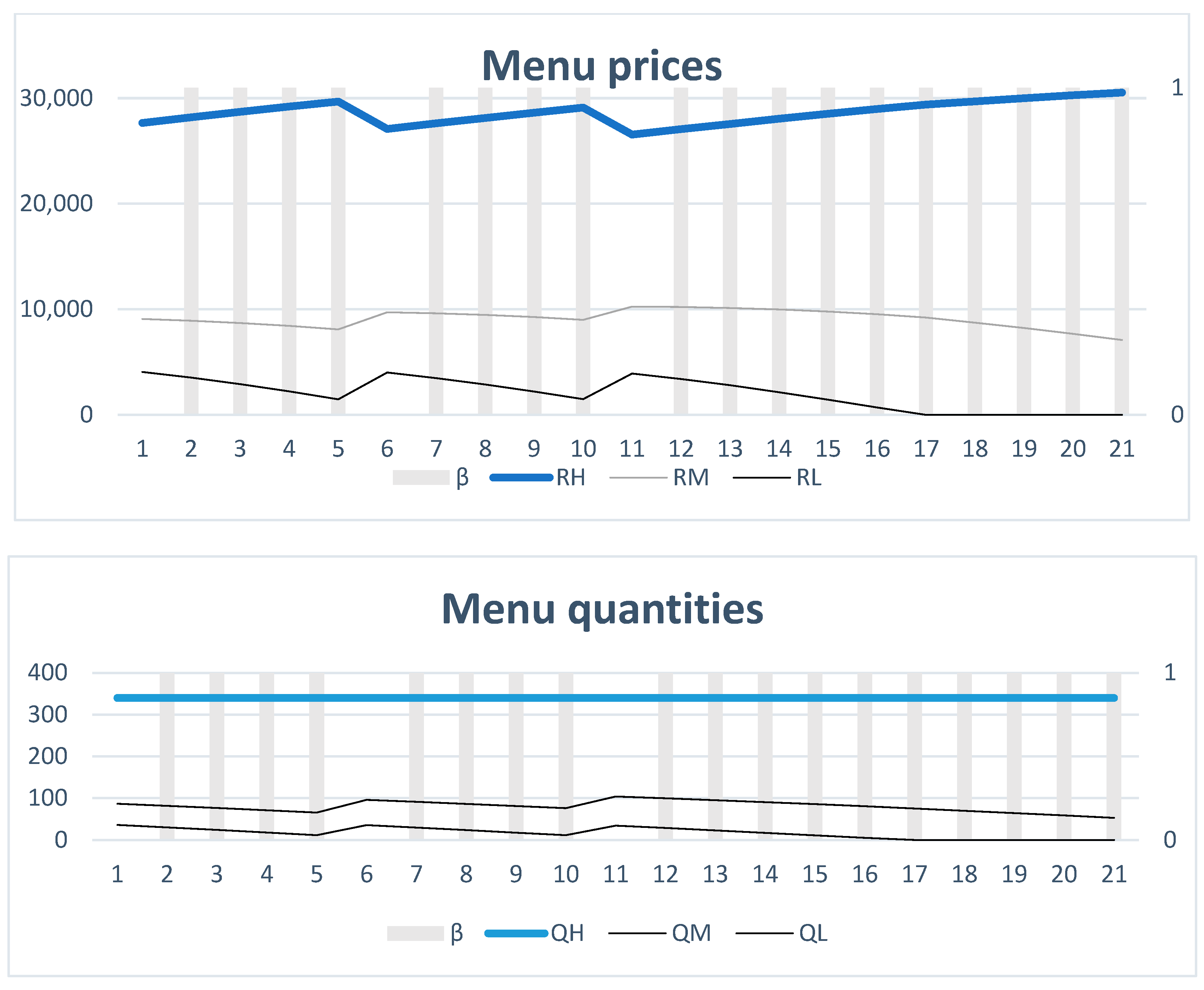
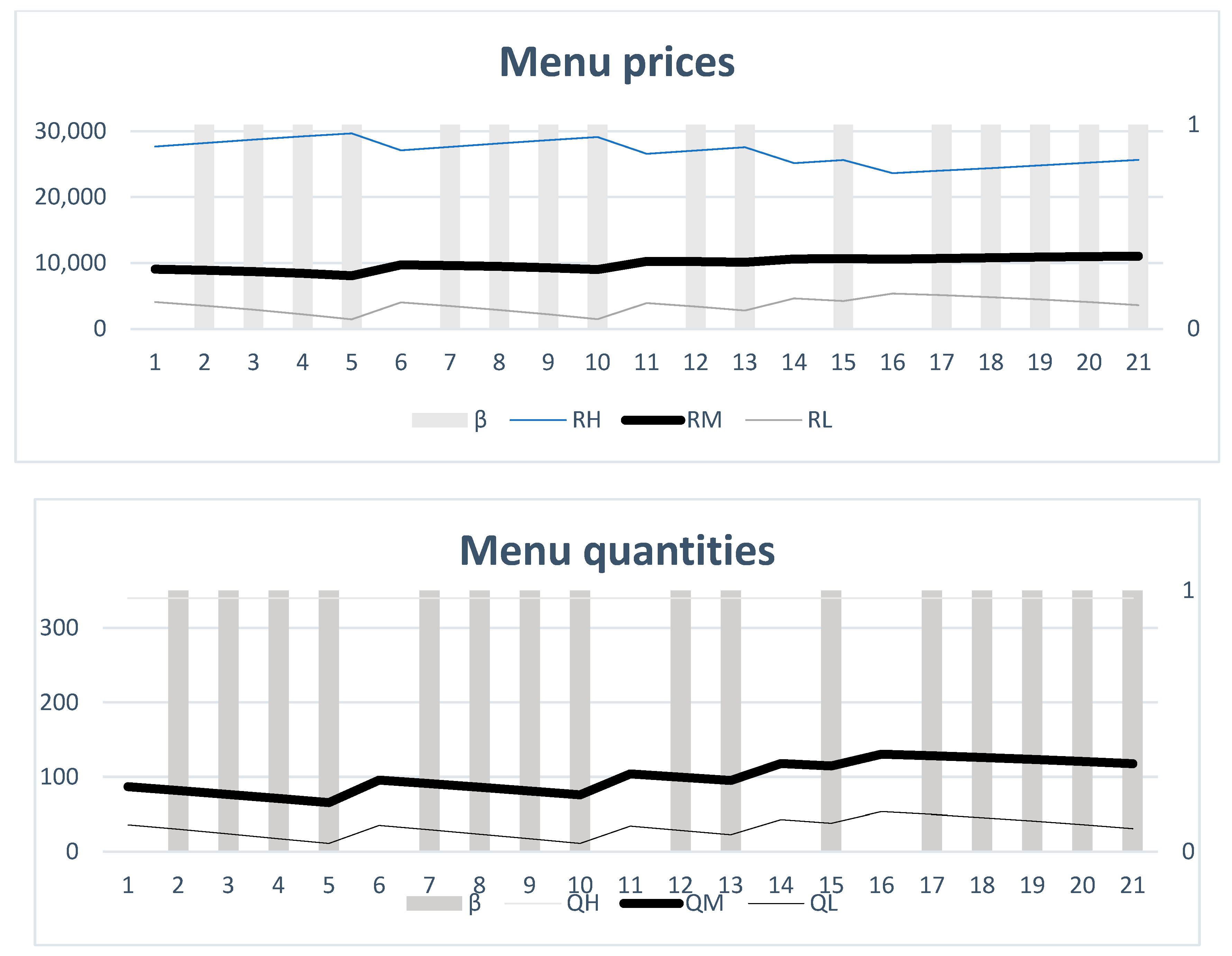
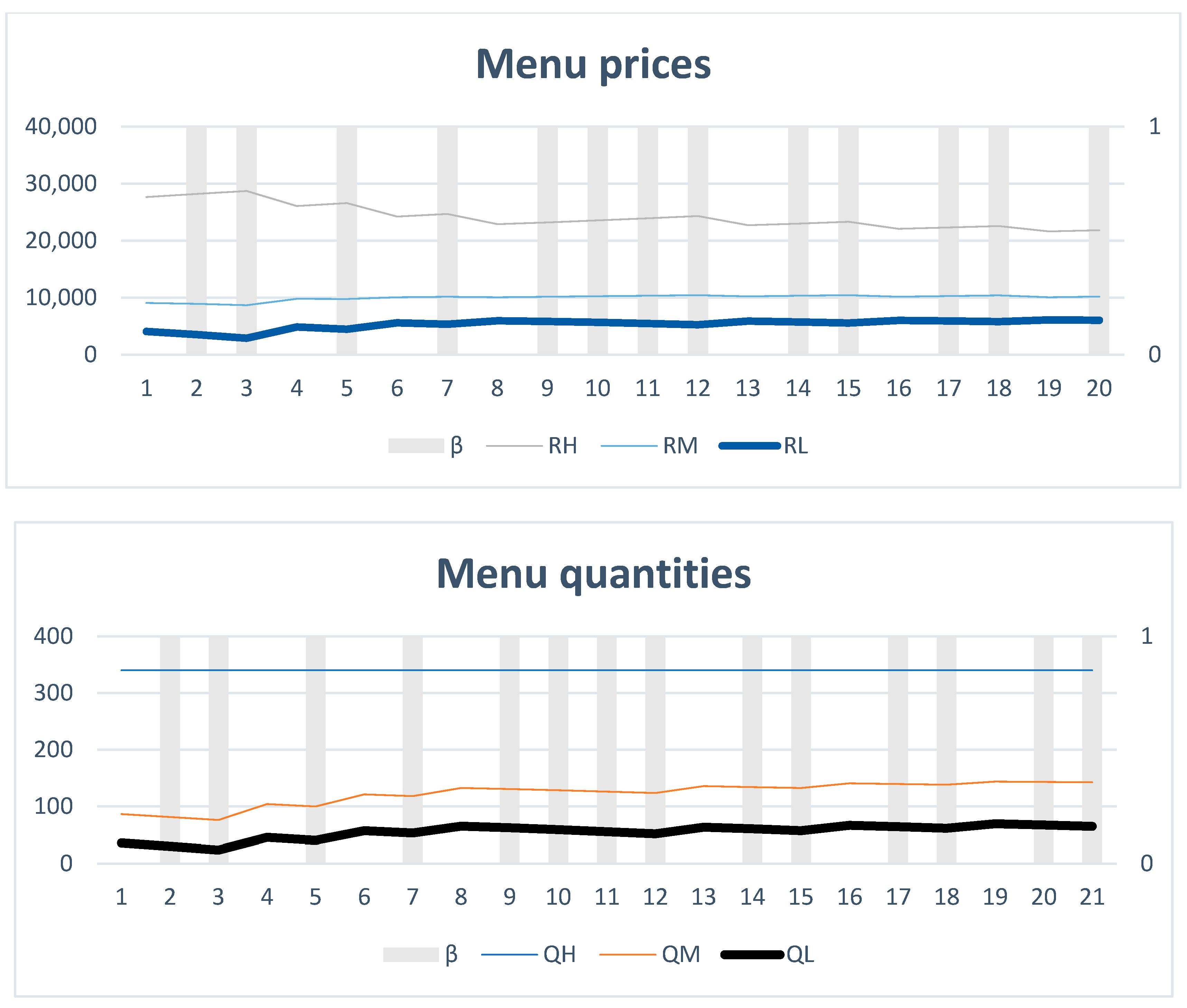
As explained in the previous section, the firm adjusts the menu prices and quantities offered to consumer i over time as the probability distribution across the consumer types changes. While Proposition 4 explains how the equilibrium values converge over time, the analysis here will show the changes from one period to another for each of the buyer types. Figure 4, Figure 5 and Figure 6 show the menu prices and quantities offered to each of the buyer types. The incentive-compatible bundle price and quantity are shown using the bold lines. In periods where ${\beta }_t$ = 0, the probability that consumer i is a low-demand-type buyer always increases, resulting in an increase in $Q_{Lt}$ and $R_{Lt}$. The effect of ${\beta }_t$ = 0 on $p_{Mt}$, $Q_{Mt}$, $R_{Mt}$ and $R_{Ht}$ is less clear, as illustrated in Propositions 1–3.

Figure 4 shows the menu of products offered to the high-demand-type buyer. The price of the high bundle is trending upward, while the other prices are trending downward as it becomes more likely that the buyer is of a high-demand type. Similarly, the quantities of the medium and the low bundles decrease as it becomes more likely the buyer is of a high-demand type. At t = 17, the firm does not offer a low bundle in the menu of choices to the high-demand-type buyer as the probability the buyer is of a low-demand type is low enough. Note that ${\beta }_6$ and ${\beta }_{11}$ are zero. In both periods, $p_{Mt}$ increases, which, in combination with the decrease in $p_{Ht}$, increases $Q_{Mt}$ (Equation (A7)). As both $Q_{Lt}$ and $Q_{Mt}$ increase, $R_{Ht}$ decreases.

The menu prices and quantities offered to the medium-demand-type buyer change over time, as shown in Figure 5. Since ${\beta }_t=1$ for t = 2 to 5, $p_{Mt}$ decreases. However, when ${\beta }_6=0$, $p_{Mt}$ increases (since $p_{L5}<p_{H5}$), which, in combination with the decline in $p_{Ht}$, increases $Q_{Mt}$. The overall effects of these changes results in a higher $R_M$ and a lower $R_H$ (see Figure 2). Similar changes take place in periods t = 11, 14 and 16, where ${\beta }_t=0$.

Figure 6 shows that ${\beta }_t$= 0 is a more frequent occurrence since this represents is a low-demand-type buyer. In those periods, $Q_L$ increases relative to the previous periods, creating an upward trend in $Q_L$ and, therefore, $R_L$. For t = 4, $p_{Mt}$ increases, while $p_{Ht}$ decreases, which increases $Q_{Mt}$. However, in t = 6, 8, 13, 16 and 19, both $p_{Mt}$ and $p_{Ht}$ decrease. The combined effect of these changes in principle is ambiguous (Equation (A7)), yet in this case it results in a higher $Q_{Mt}$. In those periods, $R_{Ht}$ decreases as both $Q_{Lt}$ and $Q_{Mt}$ increase.

5. Conclusions

This paper builds a theoretical model to analyze individualization in online markets, where firms use pricing algorithms that continuously utilize the available high-frequency market information to optimize the menu of products offered to individual consumers. Previous research analyzing online firm behavior has relied upon the established models of first-degree price discrimination models (where the firm knows the buyer type with certainty) or second-degree price discrimination models (where the firm cannot identify the buyer type), which do not capture the realities of online markets. I expand on the existing models and offer a generalized model of price discrimination that adequately models individualization in online markets. This model (1) provides an analysis of firm behavior when the firm has some, but not all, information about a buyer’s type, and (2) models firm learning as new buyer information becomes available,; and, (3) describes how the menu of products offered changes in response to this information. As the firm collects new information, it updates the probability distribution across buyer types for a given buyer through Bayesian learning and offers a product menu that is incentive-compatible.

The paper analyzes the effects of individualization on the quantities and prices offered. While it is generally understood that individualization might be useful to buyers as they are targeted with relevant information and products, this paper shows that individualization reduces consumer surplus, especially for buyers with higher demand, as it raises prices and therefore raises firm profit. While individualization skews the market surplus towards firms, it improves social welfare as firms move towards producing the socially optimal amounts. So, policymakers who aim to address the distributional consequences of individualization need to do so in a way that does not distort incentives to produce.

The extent of individualization adopted by firms will depend on the availability of relevant data on consumers and the firms’ ability to access these data, which will depend on the cost of collecting data and the dynamics of the data market. Higher data costs may reduce the extent of individualization as less information is utilized. Therefore, a future extension of this work might consider an analysis of the data market and how it can potentially affect individualization. Market competition is another factor that can potentially limit the extent of individualization by firms as firms compete and offer lower prices to attract buyers. Addressing the impact of market structure on individualization is another future area of research.