Article

Unveiling the Power of ARIMA, Support Vector and Random Forest Regressors for the Future of the Dutch Employment Market

Department of Cognitive Science and Artificial Intelligence, School of Humanities and Digital Sciences, Tilburg University, 5037 AB Tilburg, The Netherlands
*
Author to whom correspondence should be addressed.
J. Theor. Appl. Electron. Commer. Res. 2023, 18(3), 1365-1403; https://doi.org/10.3390/jtaer18030069
Submission received: 11 May 2023 / Revised: 19 July 2023 / Accepted: 4 August 2023 / Published: 8 August 2023

Abstract

:
The increasing popularity of online job vacancies and machine learning methods has raised questions about their combination to enhance our understanding of labour markets and algorithms. However, the lack of comparable studies necessitates further investigation. This research aims to explore the effectiveness of Random Forest Regressor (RFR) and Support Vector Regressor (SVR) machine learning models in predicting online job vacancies compared to the auto-regressive ARIMA method. To answer this question, detailed sub-questions are posed in relation to the sub-samples of the main data provided by Birch Consultants, an external partner originally obtained by Jobdigger. Drawing upon previous research on time-series accuracy, this study combines various approaches to benefit society and the external partner. Using the walk-forward validation method, with a 91-day expanding window, it provides precise answers to the sub-questions. Findings suggest that RFR is suitable for forecasting larger samples, while SVR is preferred due to its capability to predict small series despite relatively small scoring benefits and computational costs. Both machine learning models outperform the baseline ARIMA model in capturing complex time-series. Further research should focus on exploring advanced auto-regressive, deep learning, and hybrid models for future investigations.

1. Introduction

The labour market, encompassing worker supply and demand, holds crucial importance in modern economics. Understanding this dynamic equilibrium has become increasingly urgent. The rise of online job boards (OJBs) and online job vacancies (OJVs) has revolutionized job seeking, providing novel and robust platforms for employees. Notably, OJV data has gained significant value due to its increasing popularity [1], especially in highly developed countries like the Netherlands [2]. Consequently, leveraging OJV data for analytical and predictive purposes was proposed by [3]. As new technologies and machine learning algorithms gain traction, the question arises: Can AI effectively predict the labour market? Moreover, what is the optimal approach? Despite the proven accuracy of machine learning, there is a notable dearth of studies that combine OJB data with forecasting algorithms, leaving a substantial knowledge gap in the field [4].
This research aims to bridge the existing knowledge gap by identifying the most robust tool for accurately forecasting the number of online job vacancies in online job boards, specifically within the context of the Dutch labour market. Adopting a novel approach, the study will utilize a quarterly data feed (91 days) to forecast the intervals between each feed. The research will compare the widely employed ARIMA algorithm with the Random Forest (RF) and Support Vector Machine (SVM) methods, which have demonstrated advantages and relatively straightforward implementation for time series forecasting. By assessing the performance of these algorithms across multiple prediction tasks and setups, the study seeks to determine the optimal algorithm for specific situations and highlight their contrasting outcomes. Birch Consultants, a research and consulting company specializing in the public sector, collaboratively developed this research to analyse literature, explore potential applications, assess the database’s state, and present the following research question:
How do the performance of Support Vector Regressor and Random Forest Regressor compare to that of the widely-used ARIMA time series forecasting model in predicting the number of online job vacancies in the Netherlands?
In addition, to obtain more comprehensive answers about the performance of all three models, three sub-questions were formulated:
  • To what extent do the selected models demonstrate efficacy in predicting job vacancies categorized as “innovative” and “non-innovative” when confronted with an imbalanced dataset?
  • To what extent do the models perform in predicting a reduced number of online job vacancies, taking into consideration the required education degree?
  • To what extent does the performance of the selected models differ when the granularity of the data transitions from the national level to the provincial level?
The primary objective of this study is to identify the most suitable forecasting method for accurately predicting the number of OJVs in the Netherlands. Through a series of carefully designed sub-questions, this research aims to assess the robustness of each method while evaluating the cost–benefit trade-offs associated with transitioning from purely statistical approaches. Moreover, the experiments conducted in this study explore the impact of hyperparameter tuning on model performance and effectiveness. By conducting a comparative analysis of the ARIMA, RF, and SVM algorithms, this study not only determines the optimal method for specific scenarios but also contributes to a deeper understanding of the field as a whole. The findings of this research hold academic significance and can shed light on the effectiveness of different forecasting models. Beyond academic contributions, this study carries the potential for significant social benefits. Collaboration with Birch Consultants, a consulting company involved in this project, allows the selected model to be leveraged for predicting future OJVs. This knowledge can greatly facilitate the recruitment process by enabling companies to proactively prepare for upcoming vacancies. Furthermore, policymakers and organizations can utilize the study results to guide their own research efforts or make informed decisions on which model to employ for forecasting purposes. Ultimately, this research has practical implications that extend beyond academia, making it relevant and valuable to a wide range of stakeholders.
The rest of the paper is organized as follows: Section 2 provides an overview of state-of-the-art papers discussing demand forecasting and comparative model studies in times series domain. Section 3 describes the methodology. Section 4 presents the obtained results. In Section 5, a discussion of the obtained results is presented, while in Section 6, concluding remarks are given.

2. Related Work

This section aims to provide a comprehensive overview of the literature related to the research topic, with a particular focus on comparative studies conducted previously. Firstly, the section presents specific knowledge on labour demand forecasting, followed by a broader introduction to demand forecasting. Lastly, the research outlines time-series forecasting comparative studies, summarizing the methodological approaches employed.

2.1. Demand Forecasting

Labour market predictions, a specific form of demand forecasting centred around human workers, often emphasize transparent and qualitative methods, particularly in the public sector [5,6]. Notable institutions like the Research Centre for Education and the Labour Market in the Netherlands [7] and Monash University [8] have developed hybrid methodologies combining econometric models, exploratory data analysis, and expert judgment. Conversely, some researchers rely solely on pure statistical methods [9], considering them valuable tools for evaluating socio-economic indicators [10]. Among the various approaches, the auto-regressive model, including the widely-used ARIMA model, remains a popular choice, particularly for unemployment rate predictions [11,12,13,14,15]. Researchers have demonstrated its high accuracy with studies such as [16], which explored labour market wage forecasting using high-order ARIMA functions. This suggests that, with appropriate configurations, the auto-regressive model can yield favourable results in many scenarios. However, studies such as [17] indicate that machine learning surpasses the limitations of econometric models in terms of prediction. This claim finds support in [18], which showcased the remarkable accuracy of Random Forest (RF) in predicting the unemployment rate within the Eurozone. Furthermore, there is a growing trend of utilizing online job boards (OJBs) as a data source for calculating common labour market indicators [19]. In fact, in [20] the authors concluded that OJVs, when combined with machine learning algorithms, significantly enhance our understanding of employee demand and labour market skills. Overall, this body of research highlights the importance of considering different approaches, including hybrid methodologies, statistical models like ARIMA, and machine learning algorithms such as RF, when seeking to obtain comprehensive insights into labour market dynamics and improve predictive accuracy. Despite extensive exploration of the labour market demand in previous years, there is a notable scarcity of sources that delve into forecasting exact numbers rather than broader estimates. One noteworthy exception is a study conducted by scholars from the Norilsk State Industrial Institute [21], where they aimed to predict the number of job vacancies in the Russian arctic zone. The researchers employed ARIMA, exponential smoothing, and Neural Network (NN) models, ultimately concluding that the auto-regressive model, ARIMA, exhibited the highest accuracy among the three methods. In the broader domain of demand forecasting, machine learning algorithms are commonly utilized in complex domains where predictions are challenging due to intricate factors, as seen in energy demand forecasting studies [22,23,24]. However, in the specific context of labour market forecasting, auto-regressive models still remain prevalent [25,26]. Nevertheless, a general trend suggests that as problems become more complex, there is a greater inclination to employ deep learning methods instead of traditional approaches, despite the potential challenges of reproducibility and effectiveness [27]. The importance of incorporating lagged inputs for precise predictions in international tourism demand forecasting was underscored by a compelling study [28]. The research demonstrated that after reaching a certain point in the number of lags, the prediction error measure stabilizes, reducing the risk of overfitting. Moreover, findings on water demand in Iraq suggested that ARIMA models are proficient in effectively handling noisy raw data [29].

2.2. Comparative Models Studies in the Time Series Domain

Comparative forecasting studies of time series models constitute a vast scientific field where researchers contrast various methods for predicting time series data to identify the most suitable approach within a specific context. For instance, in the study by [30], which examined highly seasonal data, the authors demonstrated the superiority of the rolling forecast method over the direct method. Conversely, the research conducted by [31] suggested that the difference in measured error between ARIMA and the more complex SARIMAX model could be insignificant, but indicated a need for more sophisticated machine learning methods. Furthermore, the authors in [32] showcased the superior performance of Random Forest (RF) over ARIMA in short- and long-term energy load forecasting, while acknowledging the tradeoff between accuracy, complexity, and computational speed associated with the algorithms. Similarly, in the study [33], RF emerged as the preferred choice among tree-based algorithms for gold price prediction, while ARIMA also demonstrated strong performance. In another study on predicting Australia’s real house price index [34], researchers employed 47 algorithms and discovered that forecast horizons and the problem’s linearity significantly influenced the accuracy of different models for specific applications. Notably, Support Vector Regressor (SVR) emerged as the best-performing algorithm, while most machine learning algorithms outperformed Neural Networks (NN). Additionally, the effectiveness of deep learning models in comparison to traditional models for load demand forecasting was examined in the research [35]. The authors argued that the lack of explainability in deep learning models was not justified by their performance, as the tested NN algorithms exhibited similar or larger errors compared to the RF model. Additionally, scholars have investigated different methodological approaches and validation methodsAn empirical study [36] delved into the significance of validation methods and indicated that while standard cross-validation (c-v) may be suitable for certain time-series scenarios, using out-of-sample methods that maintain the temporal order of records leads to the most accurate predictions, especially for real-life data with multiple exogenous variations. Another study by the same researchers [37] indicated that forward-validation methods, particularly rolling-origin and growing-window, tend to be the most suitable for time-series forecasting. Furthermore, the study’s [38] conclusion highlighted that the optimal model selection depends on the forecast horizon since various forecast horizons correspond to different data distributions. In summary, researchers propose various theories and approaches, but the context of the prediction, data format, and potential applications remain crucial considerations. Understanding these factors is essential for selecting the most appropriate forecasting model.

3. Methodology

This section presents a comprehensive overview of the experiments conducted in this study, providing insights into the forecasting approaches employed. We begin by discussing the databases utilized and performing a thorough analysis of the job vacancy data. Subsequently, we delve into the data preprocessing steps implemented prior to the experiments. The various algorithms used in this research are then discussed in detail. Furthermore, we provide an elaborate description of the experimental setup, highlighting the validation, hyper-parameter tuning, and evaluation methods employed. Lastly, we provide a comprehensive account of the software and hardware utilized for conducting the experiment. Figure 1 illustrates the experiment pipeline for better visualization.

3.1. Data Description, Pre-Processing and Exploratory Data Analysis

This study utilizes three databases. The primary database is the job vacancy dataset, which is referred to as the main one as it serves as the input source for the forecasting models. The other two databases, obtained from the European Commission’s website, are used solely to create an innovative feature in the primary database. Moreover, exploratory data analysis forms an integral part of the initial stages of the research and facilitates the direction of subsequent actions.

3.1.1. Datasets Description

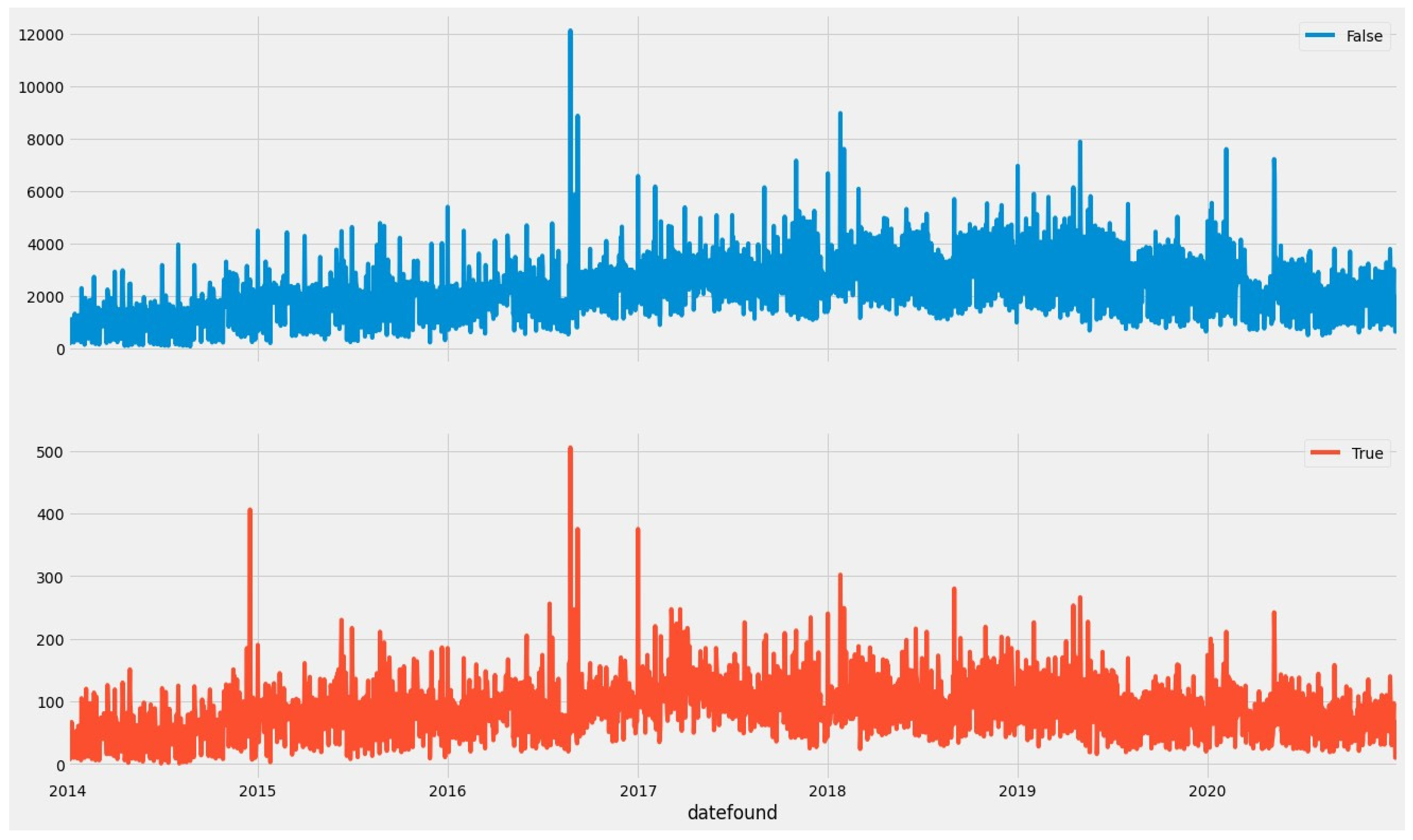
The first and primary one, referred to as the main dataset, is provided by Birch Consultants, an external partner, and originally obtained and created by Jobdigger, an international data software enterprise. It contains over 7.5 million records collected between 1 January 2014 and 31 December 2021 in the Netherlands, and includes various information on individual job offers, companies, and web-scraping attributes. To reduce the dataset size and select only the relevant variables necessary for prediction, only five features are chosen for the research purposes (see Table A1). The selection of variables is based on scientific relevance and company goals. The other two databases used to create an innovative feature in the main dataset are the EU Industrial R & D Investment Scoreboard for European companies in 2021 and the EU Industrial R & D Investment Scoreboard for Worldwide companies in 2021. These databases are published annually by the European Commission (DG Research & Innovation and DG Joint Research Centre) and collect key economic indicators for 1000 European and 2500 worldwide companies. They are used solely to select innovative companies in the main dataset. From each source, only two columns are kept: the name of the company and the R & D intensity proxy for the measured year (see Table A2 and Table A3)

3.1.2. Data Pre-Processing

The pre-processing of the job vacancy database is carried out using the Dask library, which is a Python tool for scaling data or code. Due to the large size of the main database, direct handling of it becomes infeasible, and therefore, the pre-processing step is necessary. Moreover, the absence of a large number of missing values enables straightforward treatment of unknown instances by deleting all rows where values are missing without adversely affecting the data distribution. Additionally, the pre-processing step involves transforming the educational requirement feature (see Table A4). The innovativeness feature is obtained by initially searching the European Commission databases for companies with an R & D intensity level (“The R & D intensity is the ratio of a firm’s R & D investment to its revenue for an enterprise.” [39]) of over 4%, as this percentage indicates that the company implements an innovative strategy and can be considered a pioneering enterprise [40]. The obtained companies are then searched in the main dataset, resulting in the discovery of a total of 279,533 vacancies (see Figure A1). Finally, the records are aggregated based on the features used for each forecast and day of founding, resulting in four datasets, which are presented in Table 1. The remaining pre-processing steps depend on the selected algorithms, as each requires a different input data. The baseline model, ARIMA, requires univariate input, consisting of a timestamp that places the data into the time-series domain and the observed value at that particular point, which in this case is the number of job vacancies found on a certain day. Therefore, no time-based feature extraction is applied to this model. On the other hand, the performances of RFR and SVR can be significantly improved by adding additional features [41]. As a result, the properties listed in Table 2 are obtained and transformed into dummy variables.
Additionally, rolling statistic features are included in the analysis. These properties are calculated from the number of previous time periods in the time series and are added using a window function, which is a type of calculation performed across instances related in a temporal manner. The extracted rolling features are listed in Table 3. Furthermore, a crucial practice in forecasting using machine learning and auto-regressive models is to create time lags in the time series, i.e., to shift the values forward by n-steps to establish time-dependency between records. While the baseline ARIMA model lags the data during fitting, for the other two models, lags need to be created manually. This is achieved using the auto-lag property of the ADF function from the statsmodels library. The tool is based on the Augmented Dickey–Fuller (ADF) unit root test for stationarity. Moreover, the Akaike Information Criterion (AIC) metric is chosen to determine the optimal number of lags within this function. Thus, in the SVR and RFR models, the data are shifted and the resulting outcomes are presented in Table 4.
Finally, for the input of the SVR model, the dataset needs to be scaled. Since the exploration of data distribution, explained in Section 3.1.3, indicates that the data does not follow a normal distribution, MinMaxScaler is selected as it is a robust method for these kind of values [42].

3.1.3. Exploratory Data Analysis (EDA)

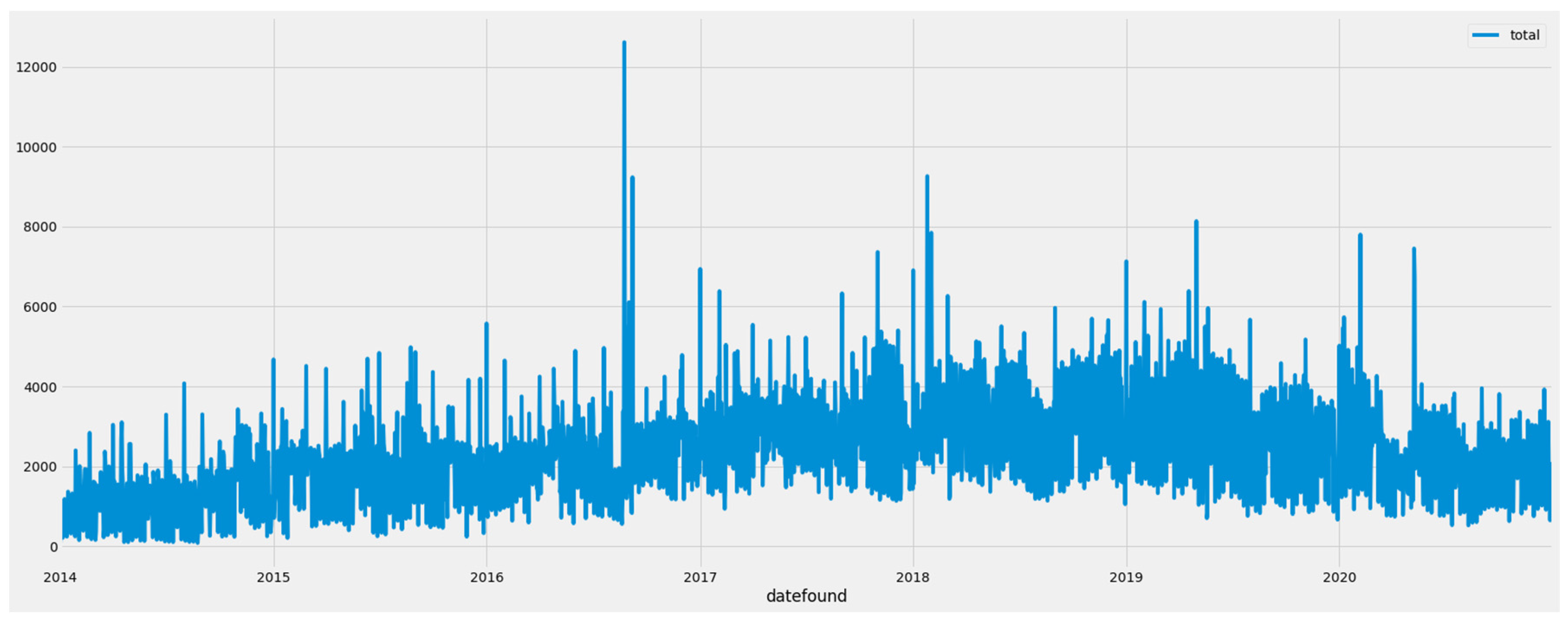
As understanding data is crucial for choosing the right tools, an exploratory data analysis is conducted. For each of the prepared forecasting datasets, a line graph visualizing the number of offers against time is created. The allocation of all openings over the training period is shown in Figure 2. Additionally, normality of the data distribution is examined. Initially, a visual inspection is conducted. The sample data values on the probability plot against the normal distribution quantiles, as shown in Figure 3, are not perfectly aligned on the line. Moreover, the kernel density estimate plot, presented in Figure 4, is not bell-shaped. Ultimately, the Wilk-Shapiro test was executed, confirming the non-normal distribution of the data (see Table A6). Based on these observations, it can be concluded that the data is not normally distributed.
Subsequently, a thorough analysis of the data graphs is conducted to investigate the stationarity of the data. The findings suggest that the data exhibits a small yet significant trend. Furthermore, a decomposition of the data illustrates not only the presence of a trend but also seasonality, as depicted in Figure 5.
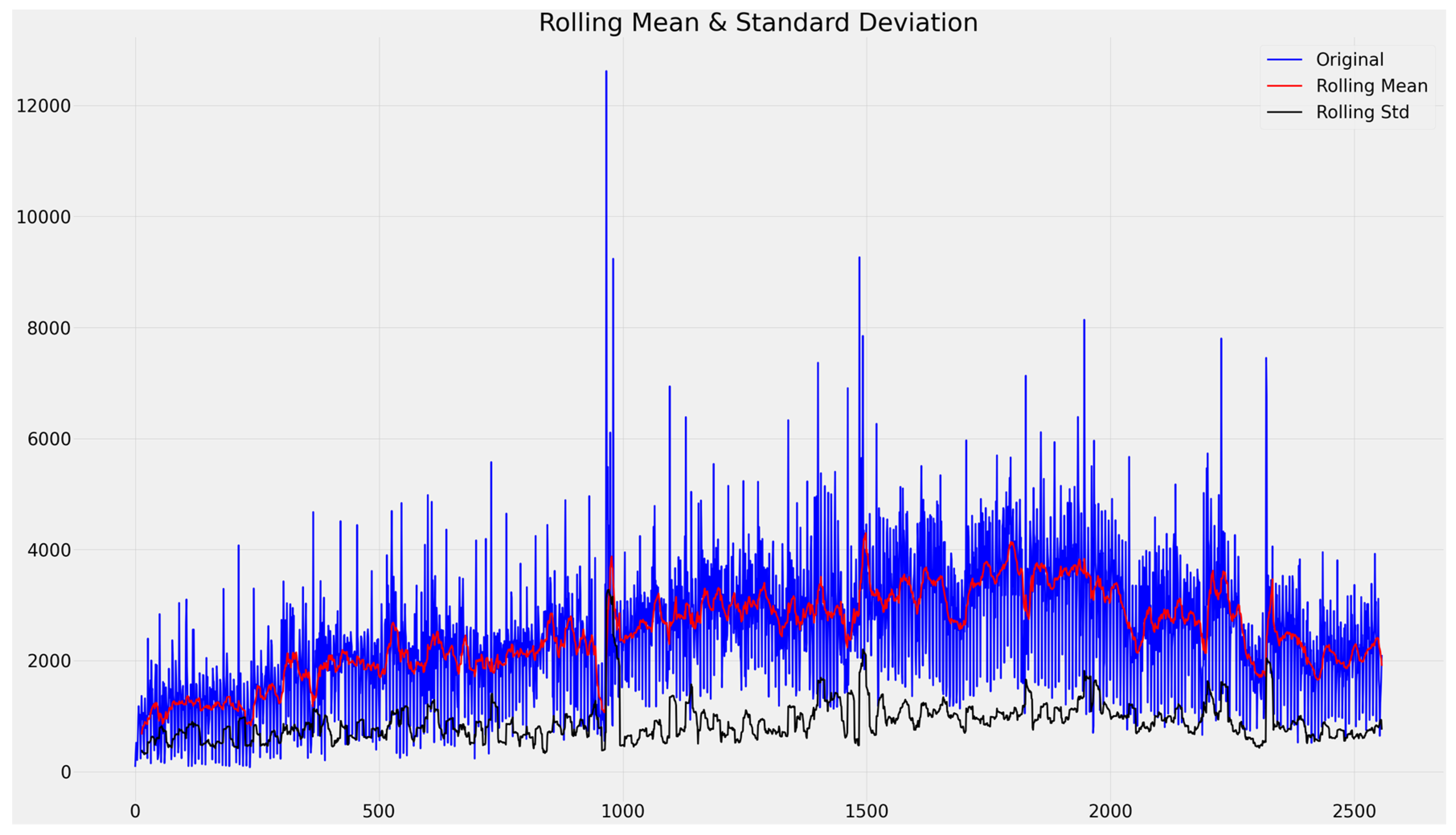
Furthermore, the rolling mean and standard deviation are explored for both Figure 6 and the decomposed data in Figure 7. After the decomposition, the first metric exhibits a more linear trend, while the second one remains inconsistent, indicating the presence of nonstationarity within the data. To back up the visual examination with statistical tests, two tests, namely Augmented Dickey–Fuller (ADF) and Kwiatkowski–Philips–Schmidt–Shin (KPSS) are conducted. The results of the former indicate the stationarity of nearly all datasets (see Table A5). However, the ndiffs function from the pmdarima library suggests a single differencing process while using the KPSS, leading to the conclusion that the null hypothesis of this test is not rejected and the data is non-stationary.

3.2. Algorithms

The objective of this study is to forecast the number of OJVs using three distinct algorithms. The baseline method, ARIMA, is compared against Random Forest and Support Vector Machine. The selection of these two methods is justified by their well-known benefits and growing popularity in the field of machine learning for time-series data. Since each algorithm utilizes a unique approach to generate predictions, the comparison of their performance resulting from this study is of great significance in evaluating their efficacy for forecasting time-related scenarios like the one presented here.

3.2.1. ARIMA

The ARIMA model, which serves as the baseline in this research, is a widely used tool in the field of time-series forecasting. The name of this algorithm is an acronym for auto-regressive (AR), integrated (I), moving average (MA). The AR component of the model is a time-series model that uses past and lagged values as inputs to the regression formula to forecast future points in subsequent time stamps. This model can be described as follows, Formula (1):
X t = i = 1 p X φ i X t i + ε t
where φ1, ..., φp are the model parameters and εt is the white noise. Moreover, the second component—I—is what sets the ARIMA model apart from the classic ARMA method. While the precursor underlying the baseline approach considers only strictly stationary data as input, the ARIMA model can handle non-stationary data by applying the differencing process, which calculates the difference between successive observations. Finally, the third component of the baseline is the moving-average (MA) model, which is a method for univariate time-series forecasting. It assumes that the output is cross-correlated with a non-identically distributed random variable. The equation for the MA model is as follows, Formula (2):
X t = μ + ε t + θ q ε t q = μ + i = 1 q θ i ε t i + ε t
The ARIMA model has three parameters, one from each element of the algorithm, namely AR (p), I (d), and MA (q). In this model, µ represents the mean of data, while θ1, ..., θq are the model parameters and εt, εt−1, ..., εt−q are the white noise errors. The d attribute denotes the number of differencing needed to obtain stationary data. The p parameter represents the number of lags used as predictors, while q refers to the number of lagged forecast errors. Several methods can be employed to estimate the algorithm parameters. For instance, visual observation of the partial autocorrelation (PACF) plot and autocorrelation function (ACF) can be used for simple time-series data. Alternatively, the Akaike Information Criterion (AIC) can be used to select the right p and q to reduce the chance of making a wrong decision. Additionally, the estimation of the parameter d can be performed visually or through the KPSS or ADF test results. The current literature suggests that the ARIMA model can be accurate in predicting future values based on past values. However, it has several limitations, such as low capabilities when forecasting complex or longer series and poor generalizability [43] (p. 273).

3.2.2. Random Forest Regressor

The Random Forest Regressor is a widely used ensemble model in the domain of regressive machine learning. This algorithm employs a specific configuration of decision trees, designed to obtain numerical outcomes. The RFR method uses the bootstrap aggregation technique, which involves creating n trees and obtaining the result by averaging the predictions made by all estimators. Additionally, when selecting a split point, the algorithm is forced to choose the best feature predictor from a limited and random sample. The RFR model has various parameters, including those related to the size of the model, such as the number of estimators, the maximum depth of each tree, and the maximum number of nodes, as well as parameters that control the learning process, such as the criterion of split, the minimum weight fraction for each leaf, or the method for calculating the number of features considered. Despite the bagging procedure, RFR may still be susceptible to overfitting and is computationally expensive. However, there are several documented benefits of using RFR, such as its robustness and flexibility. It works well even when the data contains outliers or missing values, and scaling is not necessary.

3.2.3. Support Vector Regressor

The Support Vector Regressor (SVR) is a modification of the original Support Vector Machine (SVM) that was developed specifically for predicting continuous values by identifying the best fit line. Unlike other regression algorithms that aim to minimize the difference between the predicted and actual values, SVR seeks to fit the best line within a threshold value. One of the most crucial components of the algorithm is the kernel, which is a set of mathematical functions that transforms the input into the desired format. Although the linear kernel is the most basic, many researchers prefer to use polynomials, sigmoid, or Radial Basis Function (RBF) kernels because they can overcome the linearity limitation. Another key parameter in SVR is ϵ, which represents the distance between the best fit line and ϵ-intensive bands. This parameter serves as a loss function to ensure the existence of a global minimum. The regularization parameter, C, is another important SVR parameter that determines the trade-off between achieving a small error during training and minimizing the weight norm. Finally, γ is utilized in non-linear SVR kernels to regulate the influence distance of a single instance. The unique design of SVR provides several advantages. The most notable of which is its excellent generalization capability, making it a reliable and versatile model. Additionally, the SVR algorithm is relatively flexible, allowing frequent model updates. It is also robust to outliers, although it may underperform when the data is noisy. It is important to note that SVR requires input scaling and can be computationally expensive when dealing with large datasets.

3.3. Experimental Set-Up

The selected algorithms differ significantly from each other, resulting in distinct training and tuning processes for each. While RFR and SVR share some common properties, the ARIMA method stands apart from them. However, to establish a level of comparability, the evaluation is conducted consistently, considering the algorithms’ intended real-life applications. For this research, the walk-forward validation (W-FV) with an expanding window is employed. Additionally, the RFR and SVR models undergo parameter tuning using the nested blocked c-v approach. The forecasting outcomes are primarily evaluated using the MAPE metric, with the MAE and RMSE metrics used to reinforce the reliability of the results. Furthermore, back-testing, which treats recent records as an unseen testing set, is utilized in this research. To fulfil this purpose, the test set consists of the last year of data, specifically 2021.

3.3.1. Training and Hyper-Parameter Tuning

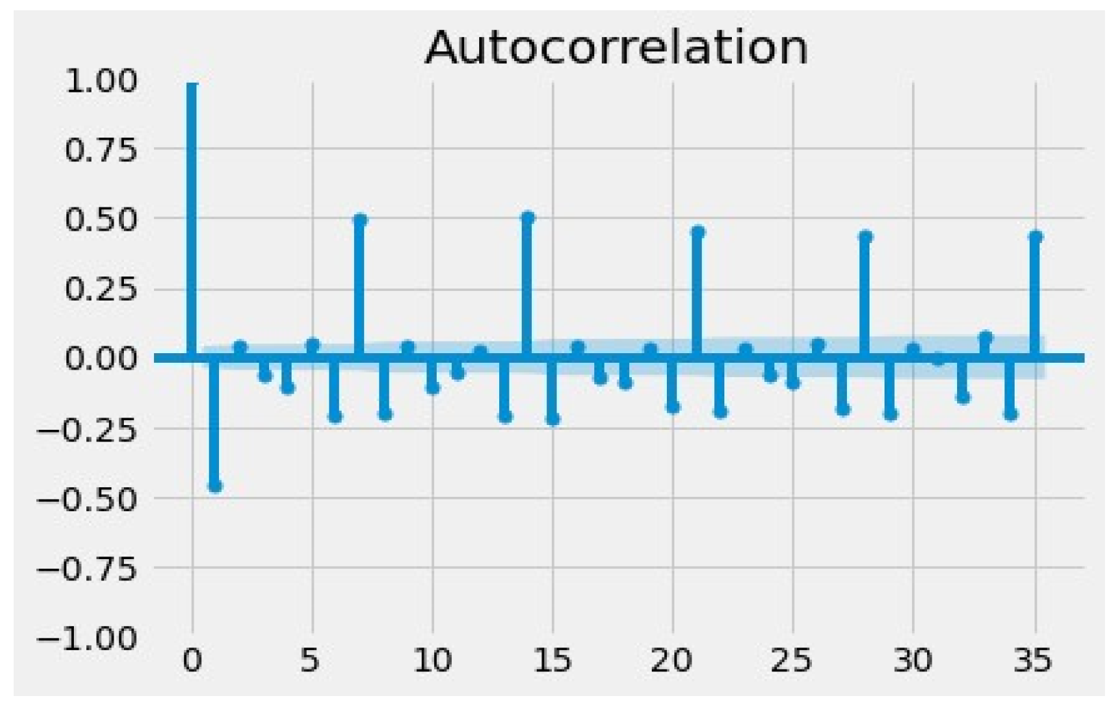
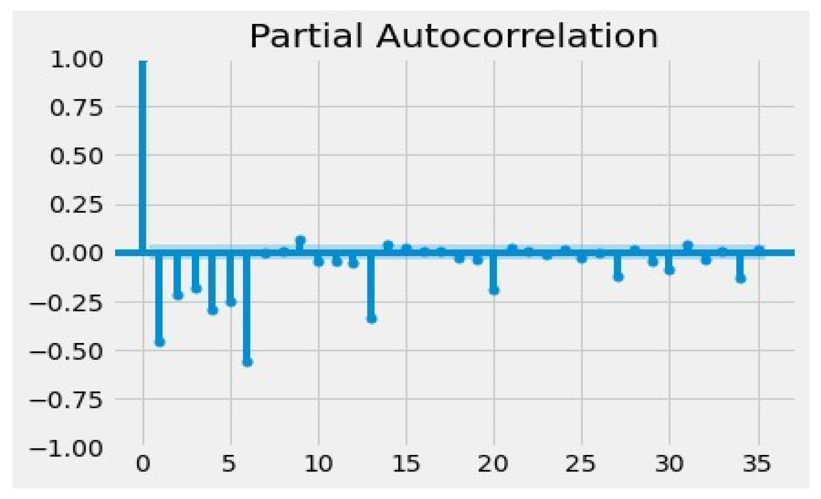
Although ARIMA parameters can be obtained by a visual examination, in this research we employed automated functions. This facilitates the selection process, and reduces the chance of a mistake, since the ACF in Figure 8 and PACF in Figure 9 are not perfectly explicit. As a result, the parameters p and q are chosen for each forecasting with reference to the results given by the auto arima method from the pmdarima library. This function fits several models and selects the best performing one in terms of the lowest AIC value. The setup of the function is shown in Table 5.
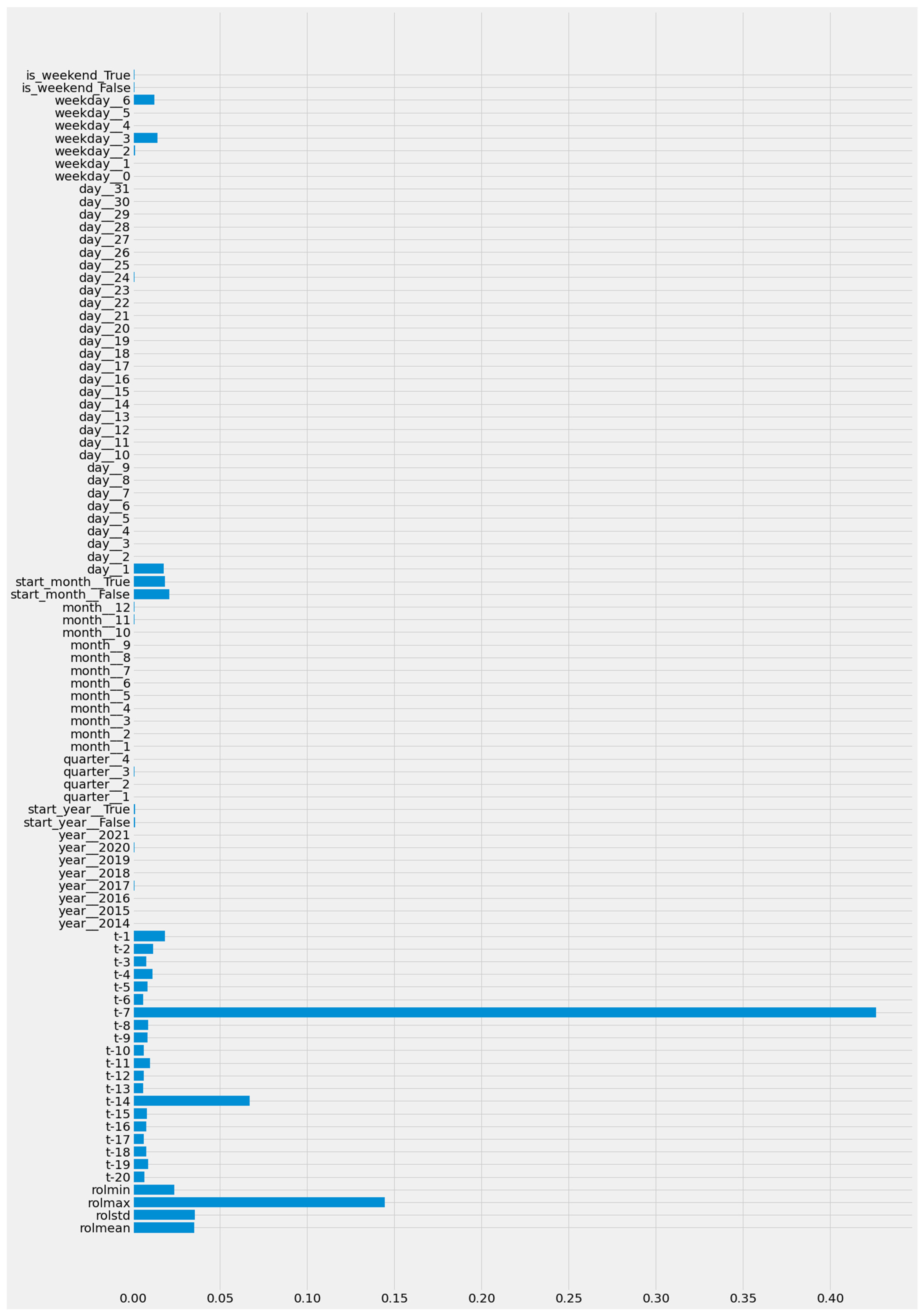
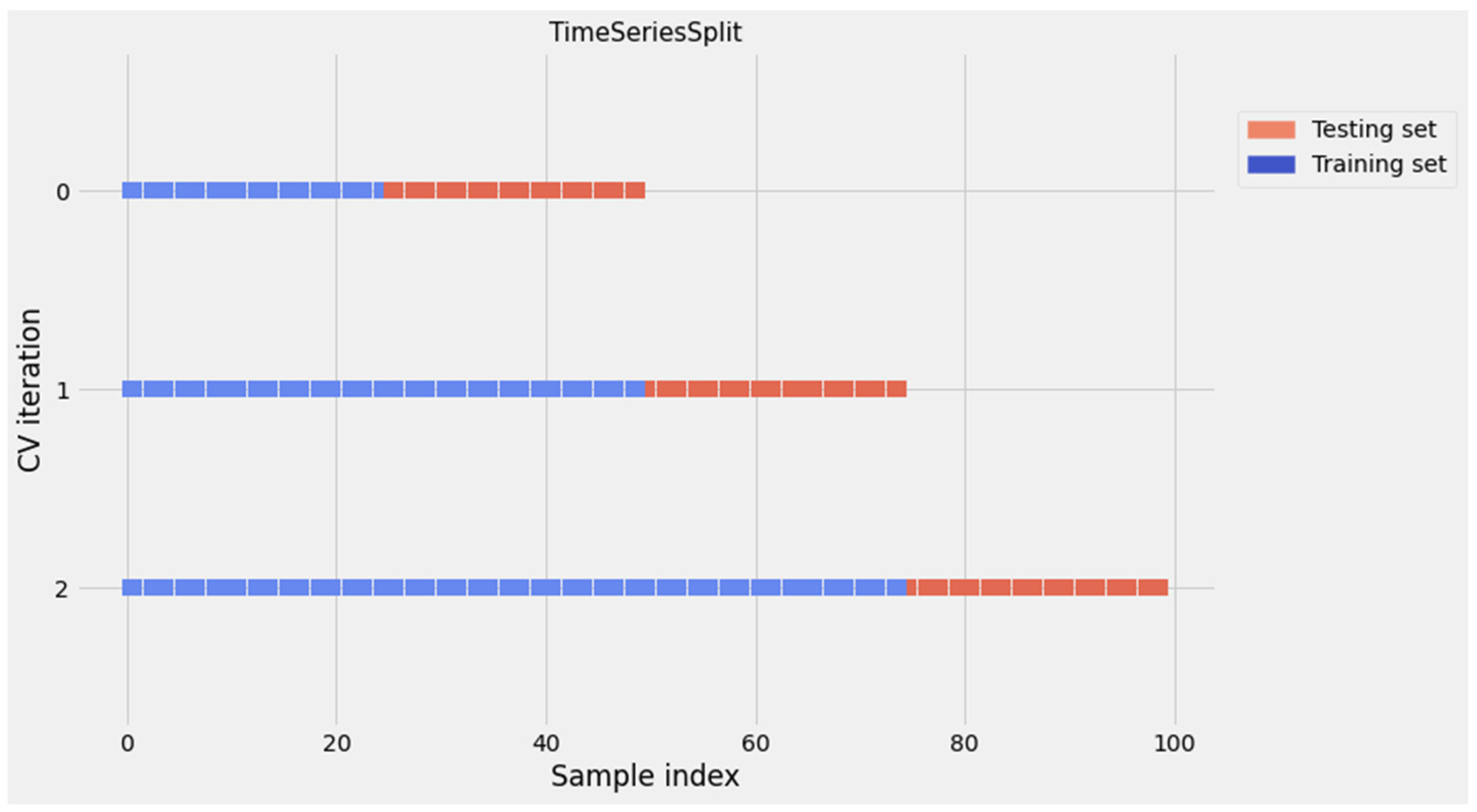
Furthermore, the Multi Output Regressor is utilized to forecast multiple series since ARIMA cannot handle more than one series at the same time. After selecting the optimal p, d, q values, the model fitting is carried out. RFR is a multivariate model, and the research exploits this advantage by using temporal-based features extracted from the data. However, the method is sensitive to the number of features, and thus Recursive Feature Elimination (RFE) is employed. RFE is a feature selection method that removes the weakest variables by fitting the model until a selected number of features is obtained. To test the overall strength of predictors on the main model, the feature importance plot is used. It is observed that around one third of all features are significant. The graph is allocated in Appendix A. Therefore, no more than 30% of all available predictors are selected for all forecastings. As consecutive forecastings have the same number of features, only multiplied by the number of series to be predicted, the same percentage is used for all forecastings. The selection steps of the function are chosen with regard to data size and possible efficiency effect. Furthermore, it is examined whether the model predicts better when the number of trees is doubled. Three model parameters are tuned, namely the maximal depth of the trees, minimal samples per leaf, and minimal sample split. The tuning is performed within a specific c-v function—Time Series Split, which is exemplified in Figure 10. Furthermore, Randomised Search, an estimator of the best model given certain parameters, is utilized. All the values selected for hyperparameter tuning are presented in Table 6.
As the generalization capabilities of the SVR model are independent of the dimensionality of the feature space, feature selection is not performed. In this model, four parameters are tuned. For the kernel, RBF and Sigmoid are chosen, as they are popular and accurate in solving complex problems. Additionally, different sizes of gamma, epsilon, and C are examined. The method of hyperparameter tuning remains the same as in RFR, i.e., nested time-series c-v with Random Search. Similarly to ARIMA, SVR cannot forecast multiple time-series simultaneously, and hence the Multi-Output Regressor is used. The last province model is compiled with over seven times the kernel cache size. All selected SVR setups are presented in Table 7.

3.3.2. Model Evaluation

The evaluation of all models is conducted in a congruous way to obtain comparable results. The year 2021 is chosen as the test set. However, instead of the standard validation process, the study uses W-FV with an expanding window. This method is an out-of-sample testing method that many regard as the gold standard, especially in the field of stock forecasting [43,44]. In principle, the technique uses past values available at a given point in time to predict the future, making it the most transposable method for real-life applications where data is periodically supplied to the model. To test how algorithms would perform in the context described above, the research uses a year-long benchmark as the test set. The expanding window implementation in the research creates five minor models, each with a 91-day forecasting horizon, and consequently, all of them have different train and test sets. An example of the validation methodology is shown in Figure 11.

3.3.3. Model Performance Metrics

This study employs three different and complementary metrics: Root Mean Squared Error (RMSE), Mean Absolute Error (MAE), and Mean Absolute Percentage Error (MAPE). RMSE is commonly used and penalizes larger errors more, which is important as MAE does not indicate the relative size of the error, making it difficult to distinguish large errors from smaller ones. Moreover, the bigger the gap between these two criteria, the more inconsistent the error size. Furthermore, MAPE is used as it is one of the most popular metrics in the time-series forecasting field and is easy to interpret, making it the main metric in this study. The metrics are obtained by comparing all predicted values for the entire year with the actual data. Additionally, the results for multi-series forecasting are averaged for better readability, although the values for each predicted series are also reported. The coefficient of determination (R2) is used to tune the hyperparameters in SVR and RFR as it is a suitable metric for the regression task in the Random Search context.

4. Results

In this section, we present the results of our experiments. Firstly, we describe and collate the results related to the forecasting of all vacancies. This part also covers the influence of hyperparameter tuning on the performance of the machine learning models. Then, we outline the results of all remaining predictions, which are aimed at answering the sub-research questions. In each of the sub-sections, we emphasize the comparison aspect of the algorithms.

4.1. Forecasting All Job Openings

After conducting the steps described in the methodology section, the models are compiled and results are obtained from them, and shown in Table 8.
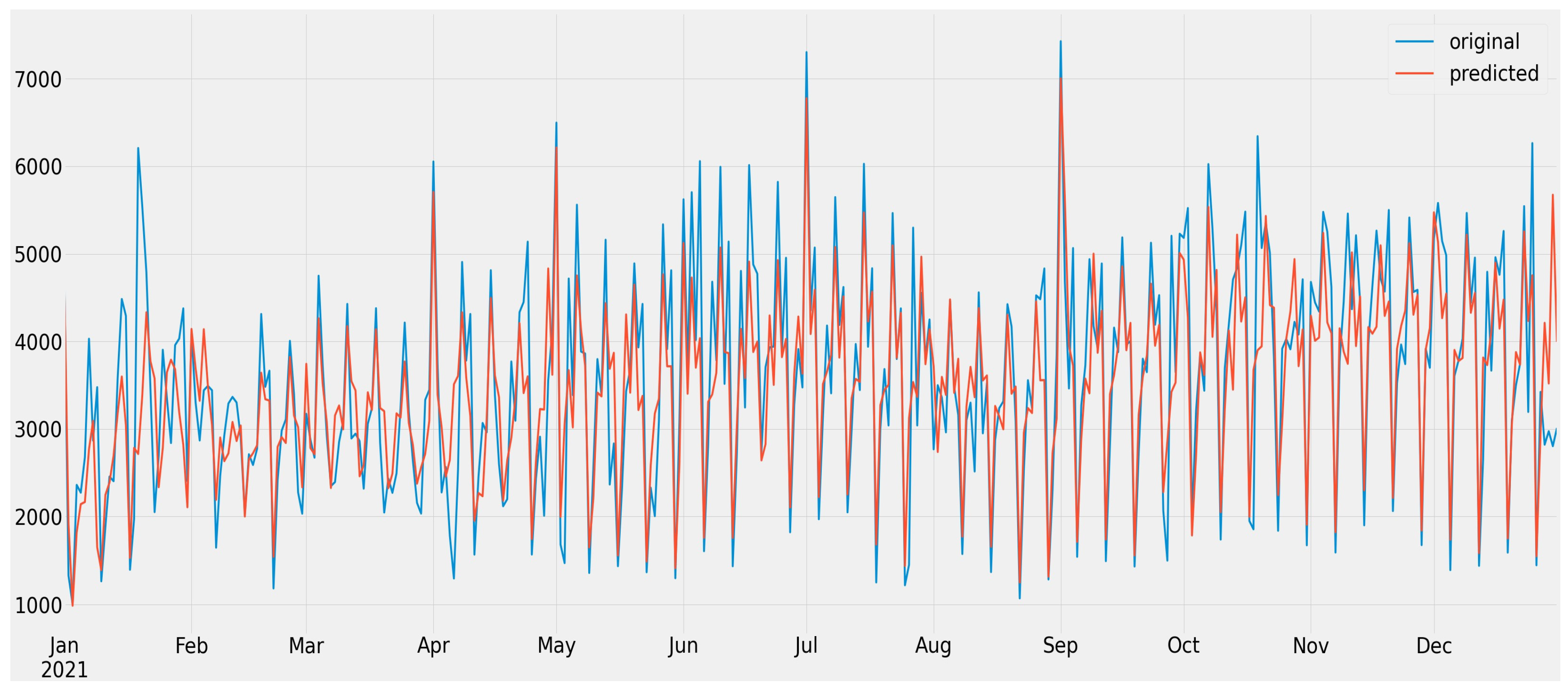
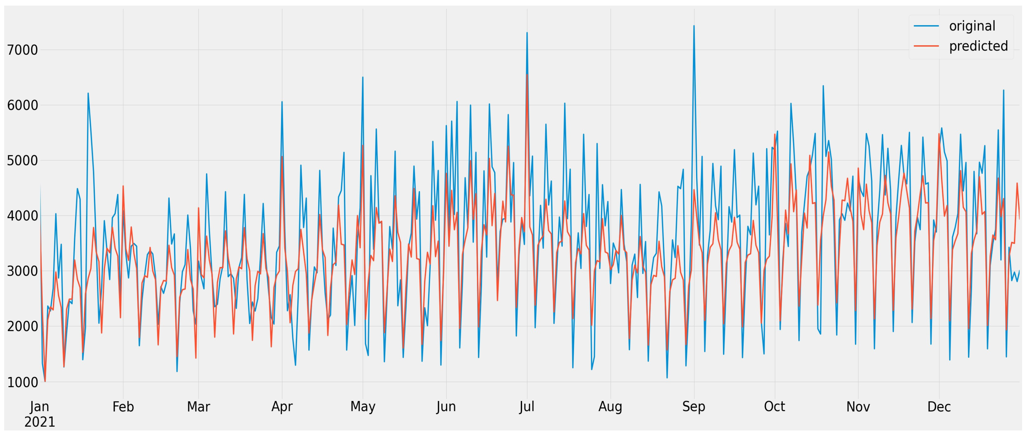
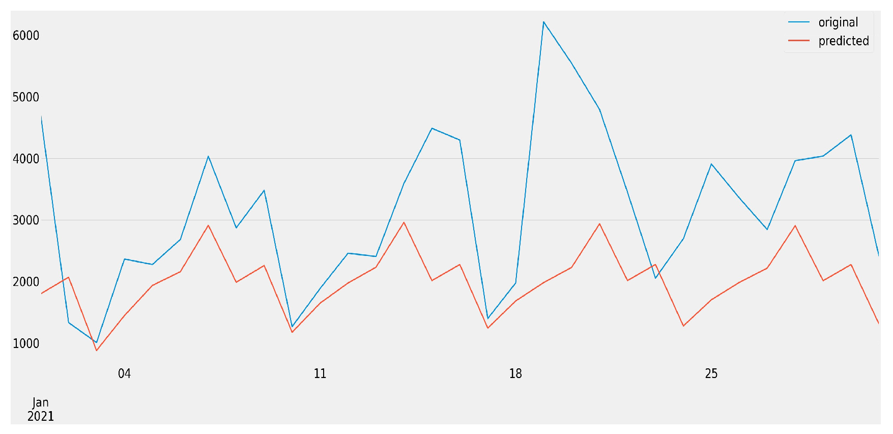
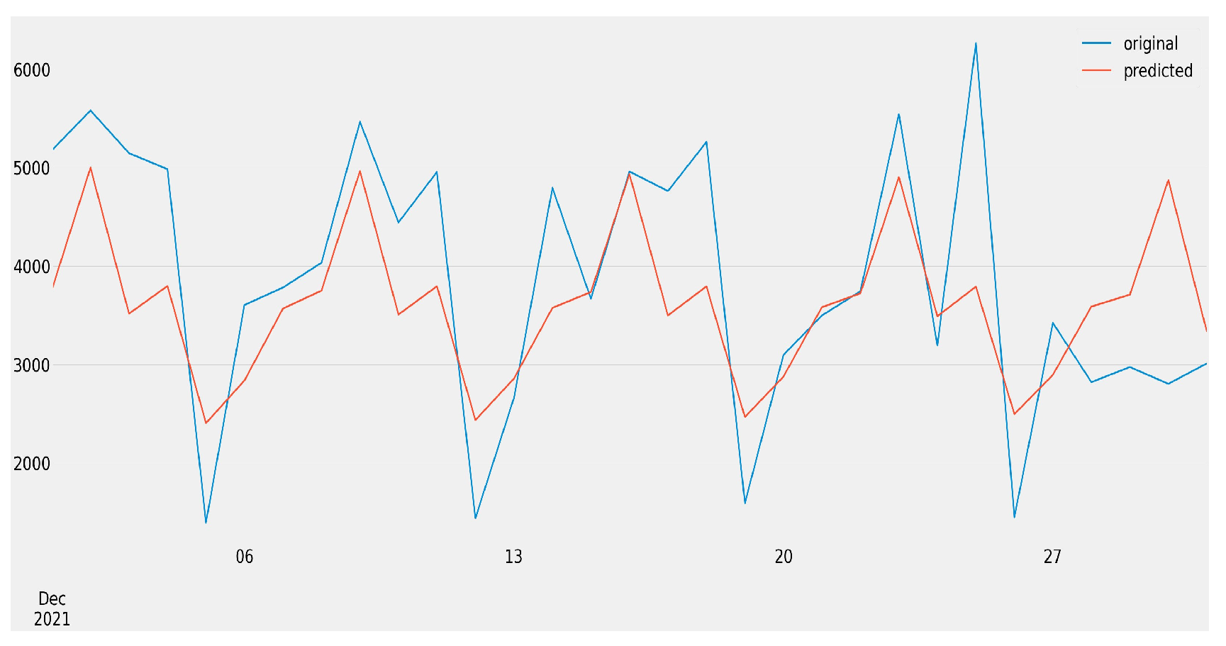
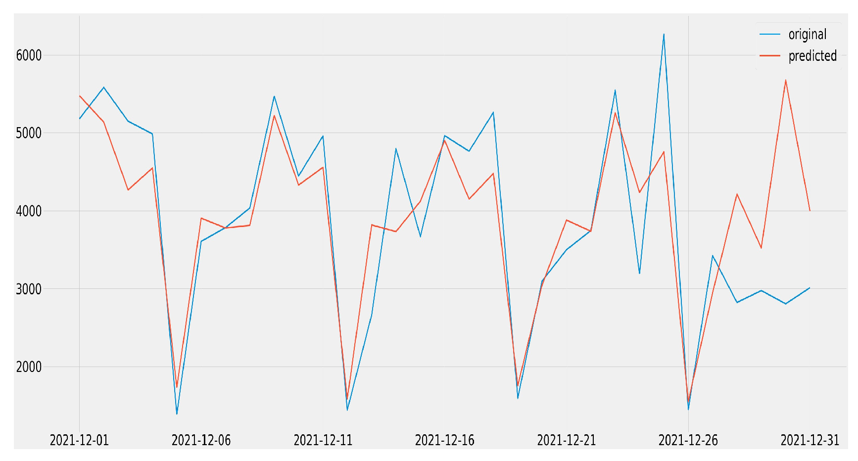
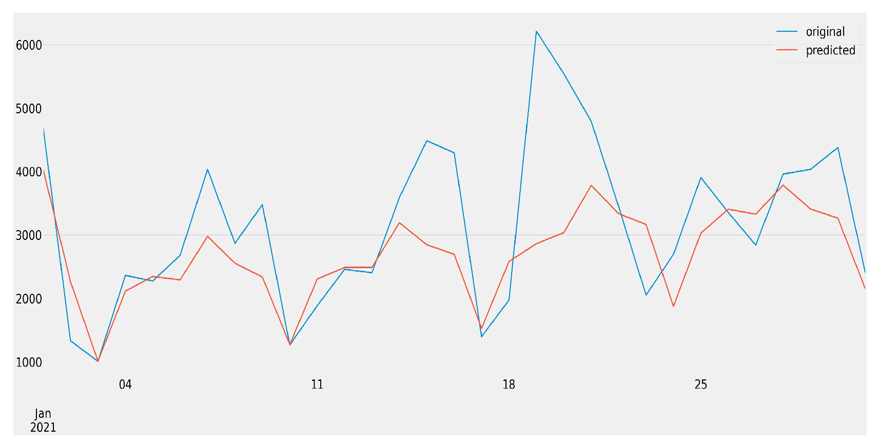
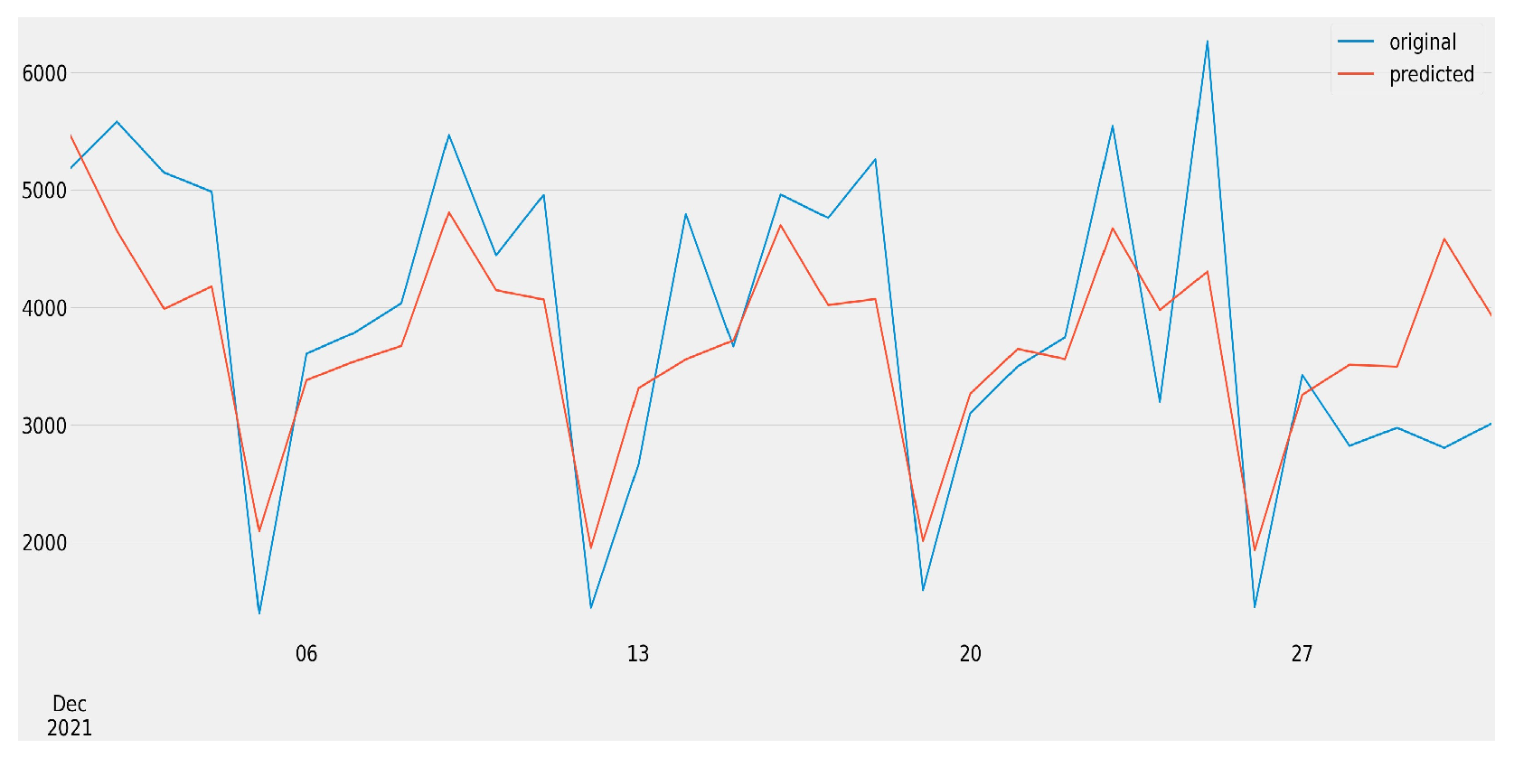
The accuracies of the models are assessed using three different metrics, all of which consistently demonstrate that the baseline model, ARIMA, is significantly less accurate compared to the other models. Among the models, RFR performs the best across all metrics, albeit with a notable increase in computation time. SVR exhibits relatively good performance with a MAPE only approximately 2% worse than the top-performing model, while compensating with faster execution speed. Visual representations in Figure 12, Figure 13 and Figure 14 further illustrate these findings by comparing the predicted values with the true values. The ARIMA model struggles to accurately predict complex and mid-term series, displaying fluctuating predictions within the same range for each forecasting window. Conversely, both RFR and SVR exhibit visually similar plots, with RFR demonstrating superior ability to capture extreme values. To obtain further insights into the forecasting results for all vacancies, additional plots are created comparing predicted values with actual values for the first and last month. Figure 15 and Figure 16 depict the baseline graph, clearly revealing that the ARIMA algorithm simply repeats the learned pattern with varying ranges for each forecasting window, leading to highly inaccurate outcomes.
The predictions made by RF are more accurate, even though it also uses a learned pattern. This is because the predictions are adjusted to fit the data better, as shown in Figure 17 and Figure 18.
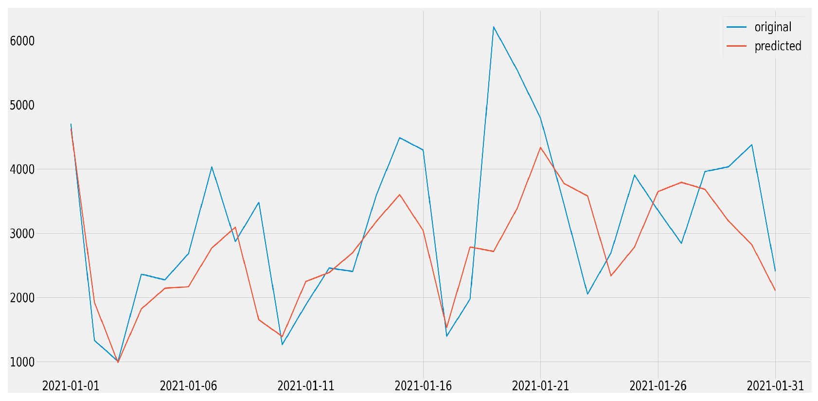
Finally, the SVR model, as shown in Figure 19 and Figure 20, exhibits a similar pattern to the tree-based models. However, it differs in that it has a greater dependence on trend or adapted seasonality.
Table 9 presents an examination of the impact of hyper-parameter tuning on the machine-learning models. The results highlight that the SVR model is particularly sensitive to the selection of hyper-parameters. After tuning, the performance of SVR significantly improves, with the errors nearly halved across all metrics. In contrast, RFR demonstrates consistent performance across various configurations, exhibiting negligible differences in the measured errors. Furthermore, when it comes to adding more predictors to the RFR model, the impact on performance is insignificant. However, it should be noted that training time doubles with the inclusion of additional predictors.
The assessment of feature importance within the primary forecasting dataset reveals the consecutive seventh lag, fourteenth lag, and rolling max variable as the most important for the model (see Figure A2).
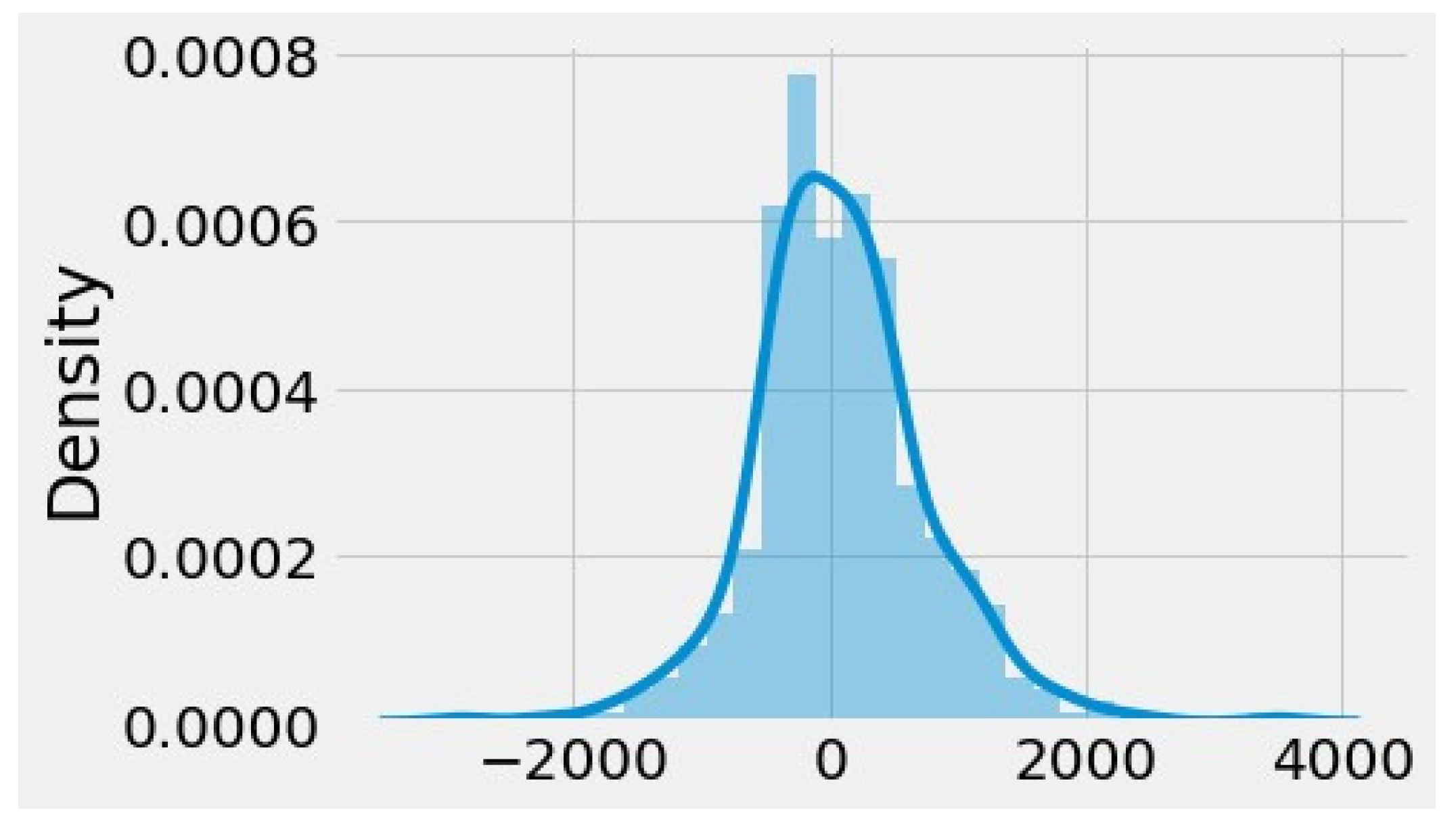
The graphs depicting the residuals of the ARIMA (see Figure A3) and SVR (see Figure A4) models are similar, with the only distinction being that the residuals of the ARIMA model are heavier-tailed. On the other hand, the residuals of the RFR model exhibit a more normal distribution (see Figure A5).
For a comprehensive grasp of our forecasting techniques, we have diligently documented the results of hyperparameter tuning for each model. The finely-tuned parameters can be examined for ARIMA (see Table A7), RFR (see Table A8), and SVR (see Table A9).

4.2. Forecasting Vacancies Split by the Innovative Feature

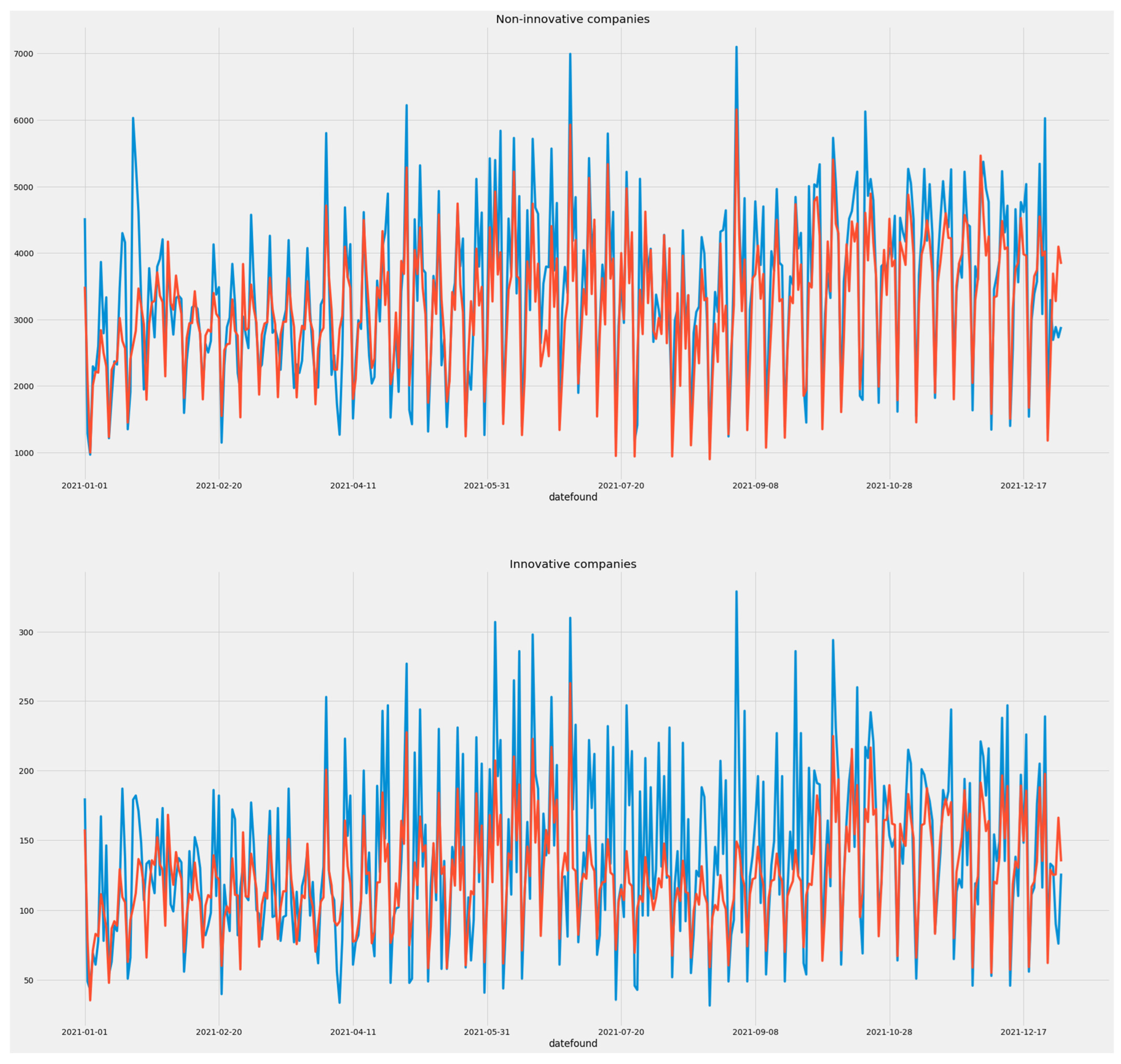
The models were also employed to forecast the number of vacancies in relation to the innovativeness feature. As presented in Table 10, ARIMA once again shows poor performance, while RFR and SVR achieve the best results. Although the performance metrics demonstrate little difference between the two models, the execution time of the algorithms varies considerably. Specifically, SVR outperforms its competitors by compiling in under a minute. The detailed outcomes for all three models can be found in a single table (see Table A10), providing a cohesive perspective on the results.
After analysing the plots of predicted versus actual values (see Figure A6, Figure A7 and Figure A8), it can be concluded that ARIMA fails to accurately forecast both innovative and noninnovative job openings. The method exhibits a lack of predictive ability, with forecasts fluctuating imprecisely for about two weeks, followed by a straight line. On the other hand, the machine learning-based models perform significantly better. Among them, SVR emerges as the best model, outperforming RFR by a small margin. Specifically, it achieves significantly better predictions over the entire period for the smaller (i.e., innovative) sample, except for the third forecasting window, where the model’s error is high.

4.3. Forecasting Vacancies by Educational Requirements

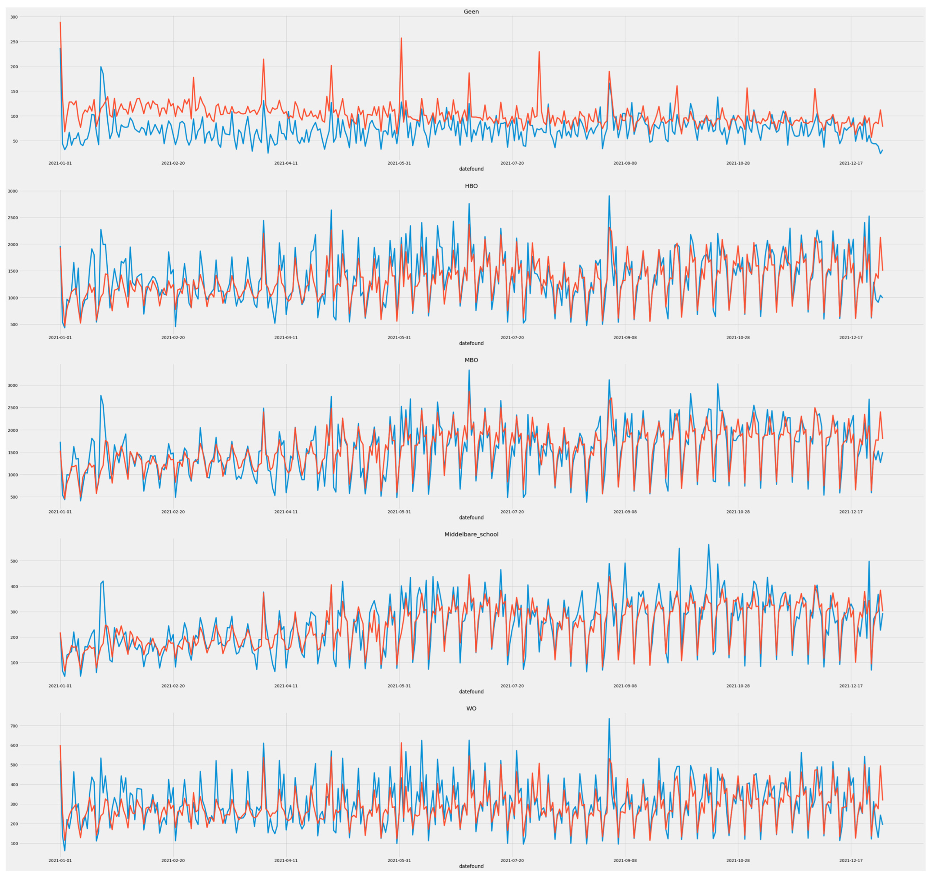
Consistently, as shown in Table 11, ARIMA demonstrates the poorest forecasting performance with results averaged across the entire series. On the other hand, SVR achieves the highest scores, with RFR predictions being extremely close, with the exception of two forecasting levels—namely WO and, more notably, Geen—where RFR fails to make accurate predictions with MAPE exceeding 50%. Once again, SVR outperforms its competitors in terms of computational speed, completing the task in around 3 min, while its rivals require either 4 times (ARIMA) or almost 16 times (RFR) more, in terms of additional time.
The conclusions drawn from the analysis are supported by the visual inspection of the predicted versus actual vacancies plots (see Figure A9, Figure A10 and Figure A11). Consistent with the previous findings, ARIMA fails to capture the trend and seasonality in most series, with the exception of the HBO series, which is the only one to achieve a MAPE below 30% in this model. RFR exhibits good performance in most series, except for the Geen series. On the other hand, SVR predicts all series accurately, but like its counterparts, performs poorly on the Geen series. The detailed outcomes of this forecasting are showcased individually for each model: ARIMA (see Table A11, Figure A9), RFR (see Table A12, Figure A10), and SVR (see Table A13, Figure A11).

4.4. Forecasting Job Openings by Provinces

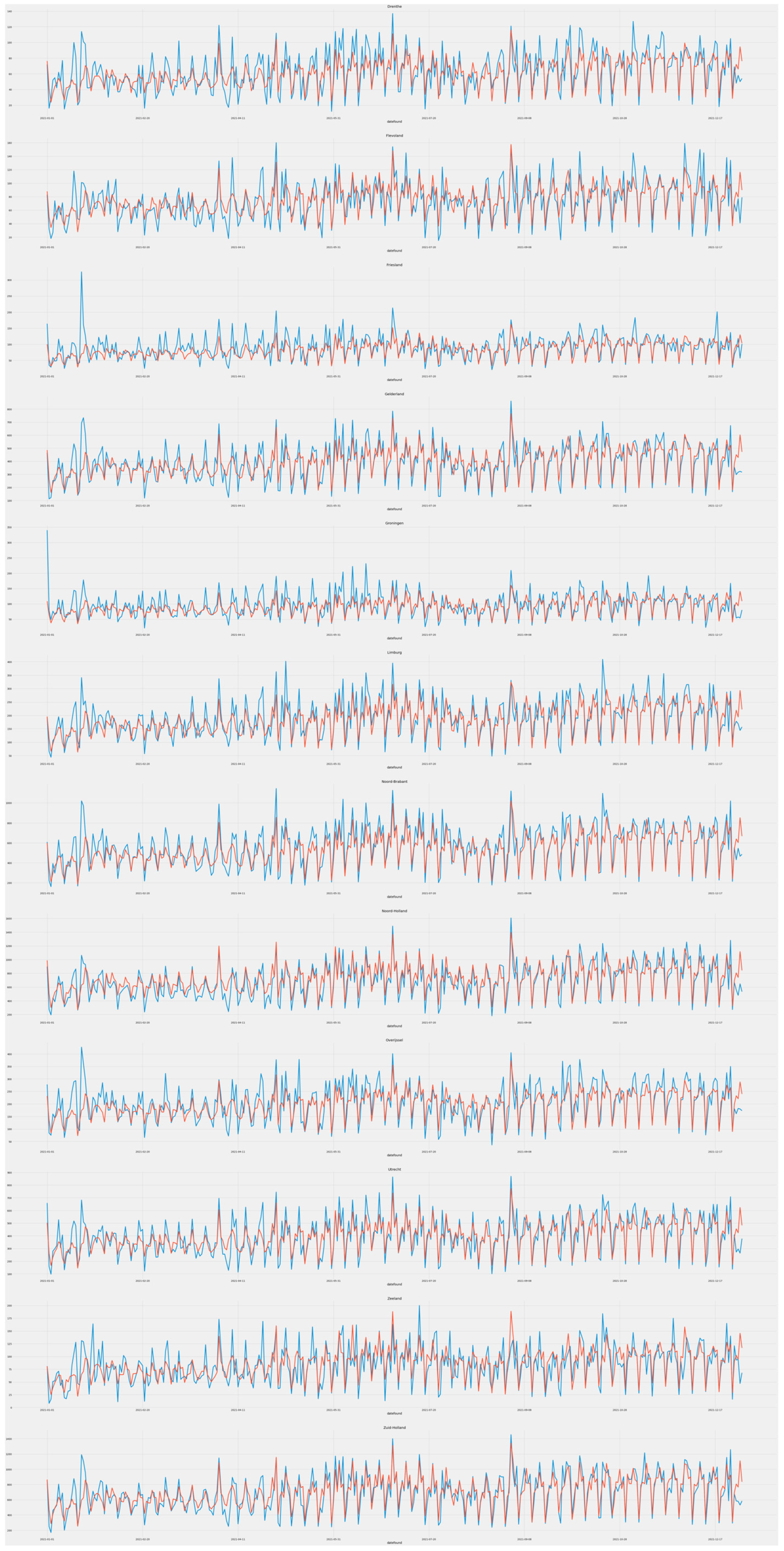
Lastly, forecasting of the number of vacancies by province is conducted and the general results are delineated in Table 12. ARIMA presents noticeably the worst performance on all three metrics. Thereupon, it is worth mentioning that, this time, three forecasted series out of twelve can be considered as a working ones, i.e., Limburg, Nord Brabant and Utrecht. The SVR model seems to be by far the best method for the scenario. In all series, it predicts better than RFR and consecutively ARIMA. The precise outcomes table can be found for all three models, i.e., ARIMA (see Table A14, Figure A12), RFR (see Table A15, Figure A13), SVR (see Table A16, Figure A14).
Table 12 displays the efficiency of the models in terms of time, with SVR being the fastest, taking under a quarter of a minute, while RFR needs over an hour more. The compilation time of ARIMA depends on finding the right parameters rather than the actual prediction, hence as the number of series grows, the time increases to around half an hour. Additionally, the table also shows the general performance metrics of each model. SVR outperforms both RFR and ARIMA on all series. Only three forecasted series, namely Limburg, Nord Brabant, and Utrecht, can be considered as working ones. SVR demonstrates significantly better predictions than its rivals. The visual examination of the figures (see Figure A12, Figure A13 and Figure A14) confirms that ARIMA forecasts correctly in the three above-mentioned provinces, but poorly, failing to capture trend or seasonality in other cases. While RFR struggles, especially in predicting the province of Zeeland, SVR performs better, even with a very small value. Graphs showing predictions of each algorithm again, and the true values, are shown in Appendix A.

5. Discussion

This section presents the experimental results by addressing the research questions outlined in the introduction. The comparison of three algorithms reveals that the baseline model performs poorly for the main research question posed in this research with a MAPE of approximately 26%. Its inadequacy stems from its inability to effectively capture the complexity of the time series, relying on a single learned fluctuation while the data is more intricate. This finding aligns with a previous study by [45], where ARIMA also struggled to predict complex load forecasting scenarios. In contrast, the RFR model outperforms the others in this scenario, achieving a MAPE of around 15.7%. However, hyper-parameter tuning does not significantly improve its performance, as observed in previous research by [46,47]. The SVR model, while significantly faster than RFR, delivers comparable outcomes with MAPEs of approximately 15.7% vs. 17.9%, respectively. Tuning is crucial for SVR, enhancing precision by approximately twofold across all evaluated metrics, consistent with previous research by [48]. However, the SVR model faces challenges with extreme values, as highlighted in a study by [49], resulting in lower accuracy for points significantly below the median. Examining the forecast residuals’ distributions, the RFR model demonstrates the most precise predictions. In conclusion, RFR is the preferred model for this application, prioritizing accuracy over time-effectiveness. The baseline model is outperformed by both machine learning algorithms and is unsuitable for extended forecasting. This finding supports the earlier assumption by [50] that the length of the forecasting horizon significantly impacts the algorithm, as enlarging the window leads to poorer ARIMA results. Although the SVR method performs relatively well and has faster computation time compared to RFR, it struggles with abnormal values. Therefore, SVR can be considered as an alternative when time-efficiency is a concern.
In examining the precision of the models in scenarios with unbalanced samples, the baseline model performs poorly, displaying the lowest performance with an average MAPE of approximately 38% across both series. Additionally, the baseline model produces linear results, suggesting that the best predictions are merely straight lines without capturing trend or seasonality. On the other hand, among the two machine learning-based algorithms, SVR is the preferred choice. It not only exhibits slightly better overall performance (18.4% vs. 19.8%), but also demonstrates superior results in predicting smaller samples. Moreover, SVR is significantly more time-efficient compared to RFR, requiring around 14 times less compilation time.
To further reinforce the examination of predicting smaller numbers using the compared algorithms, it can be concluded that the baseline model once again performs the worst, failing to capture important components and resulting in an average MAPE of 33.8%. In terms of the machine learning algorithms, SVR outperforms its main rival, RFR, by approximately 6% in MAPE (19.3% vs. 25.9%). Additionally, the issue of time-effectiveness needs to be considered. While SVR completes the process in just 3 min, RFR takes more than 15 times longer.
In summary, SVR not only demonstrates the best performance but also requires the least amount of time among the compared algorithms. Lastly, in addressing the final sub-question of obtaining results from both smaller and larger series simultaneously, the comparison between algorithms remains consistently focused on machine learning models. The baseline model again exhibits the worst performance with a MAPE of 35.3%. However, in this case, the baseline model produces tolerable outcomes in three out of twelve series, raising the question of its potential in more suitable circumstances. In this forecasting scenario, SVR outshines RFR, achieving an approximate MAPE of 15.4% compared to around 21.6% for RFR. Not only does the kernel-based model significantly outperform RFR in all predictions, but it is also several times faster.
To summarise the answers given to the above-posed questions—in the scenarios presented, SVR is the most optimal algorithm choice and therefore, the more data which is augmented, the better results the model yields. Thereupon, there is a need for thoroughgoing hyper-parameter tuning, as the influence of this step is substantial in the research experiments. RFR can be considered as an alternative for predicting larger samples; nevertheless, the computational costs should be kept in mind. Finally, the baseline is outperformed in this study by both machine learning algorithms. It can be concluded that it is not suitable for the given situations, but nonetheless may be more useful when forecasting shorter periods of time. Additionally, MAE and RMSE measured performance in a parallel way, i.e., there was no deviation providing an extra insight into the results.
Finally, the findings of this research indicate that machine learning algorithms, especially SVR, are useful when forecasting this particular OJB in a periodic manner. Moreover, with an averaged MAPE below 20%, the created models are suitable for the actual data prediction.

5.1. Limitations

This paper acknowledges several limitations that should be mentioned. Firstly, the models are trained using data spanning every 91 days, and the testing data covers 365 days, resulting in the last (5th) forecasting period consisting of only one day. Although this does not negatively impact the final results, as metrics are calculated for all predictions against the true values, it may introduce inconsistencies. Additionally, the examination of hyper-parameter tuning may not always be sufficient to determine whether the RFR model cannot be effectively tuned with this data or if the parameters were simply poorly chosen. While previous studies also highlight the relatively low significance of this aspect for the algorithm, it is important to consider this limitation. Furthermore, this study employs a standard computer, and the effectiveness of the models, particularly the more computationally intensive ones, may not present a significant obstacle for companies or other entities utilizing more efficient measures.

5.2. Future Research

The authors of this research suggest continuing the research by enhancing the scope of this study. In particular, new studies should focus on exploring the capabilities of the models compared in different experimental setups. The types and sizes of windows should be checked, since the influence of these components on the algorithms in the foregoing studies is established as more than crucial. It is also suggested to check whether more advanced models like SARIMA or SARIMAX would overcome the obstacles faced by ARIMA and provide a better baseline. Moreover, it is recommended to examine more hyper-parameter configurations to address one of the study’s limitations and to determine whether hyper-parameter tuning is indeed unprofitable for RFR. Additionally, it may be beneficial to explore new methods of searching for the best parameters in the model, similar to those examined in the study by [51].

6. Conclusions

The primary objective of this research was to identify the optimal model for forecasting the number of online job vacancies in the Netherlands on a quarterly basis (each quarter consisting of 91 days), utilizing a dataset provided by Birch Consultants. The study focused on comparing three algorithms: ARIMA, RFR, and SVR. To ensure the relevance to potential applications, the experiments were conducted using an expanding window approach. The findings of this study suggest that SVR is the most suitable algorithm for such a task. Although it performed slightly worse than RFR with larger sample sizes, SVR demonstrated superior performance with smaller samples and exhibited significantly faster computation time. Both SVR and RFR outperformed the baseline model, highlighting that ARIMA is not suitable for accurately forecasting such extended and complex time series. These results underscore the significance of further research to comprehensively understand the forecasting of online job vacancies and the associated algorithms. By delving deeper into this subject matter, a more complete understanding can be achieved, thus enabling improved forecasting capabilities and algorithm selection.

Author Contributions

Conceptualization, P.G., B.Č. and N.R. methodology, P.G.; validation, P.G., B.Č. and N.R.; formal analysis, P.G.; investigation, P.G.; resources, P.G.; data curation, P.G.; writing—original draft preparation, P.G.; writing—review and editing, B.Č. and N.R.; visualization, P.G.; supervision, B.Č.; project administration, B.Č. and N.R.; funding acquisition, N.R. All authors have read and agreed to the published version of the manuscript.

Funding

This research received no external funding.

Institutional Review Board Statement

The research did not required ethical approval since it did not involved human or animal participants. The original owner of the data used in this research retains ownership of the data during and after its completion.

Data Availability Statement

Work on this study did not involve collecting data from human participants or animals. The original owner of the data used in this study retains ownership of the data. The authors of this study acknowledge that they do not have any legal claim to these data. The code used in this study is not publicly available due to NDA (Non-Disclosure Agreement).

Acknowledgments

The authors would like to thank the whole Birch Consultants company and Jobdigger for providing the data and, consequently, creating the opportunity to carry out this study.

Conflicts of Interest

The authors declare that they have no known competing financial interest or personal relationships that could have appeared to influence the work reported in this paper.

Appendix A

Table A1. Table presents the main database features.
All available features in the main database
organization name, organization name generalized,
education degree minimum required detailed, education degree minimum required, education degree generalized, education degree,
Industry code, industry description, date found, date deactivated, closing date, starting date, active weeks,
organization place, organization_id, nr of employees
physical location municipality, physical location place,
physical location province, jdcocode,
jdcodescription, jdcoisco, position title, position title cleaned, selected text
Table A2. Table presents the Worldwide sub-database features.
All available features in the EU Industrial R&D Investment Scoreboard for the Worldwide companies for 2021 database
World rank, Company, Country, Region,
Industry-ICB3 sector name, R&D 2020 (EUR million), R&D one-year growth (%), Net sales (EUR million), Net sales one-year growth (%), R&D intensity (%), Capex (EUR million), Capex one-year growth (%), Capex intensity (%), Op.profits (EUR million), Op.profits one-year growth (%),
Profitability (%), Employees, Employees one-year growth (%),
Market cap (EUR million), Market cap one-year growth (%)
Table A3. Table presents the EU sub-database features.
All available features in the EU Industrial R&D Investment
Scoreboard for the European companies for 2021 database
EU rank, Company, Country, Region,
Industry-ICB3 sector name, R&D 2020 (EUR million), R&D one-year growth (%),
Net sales (EUR million), Net sales one-year growth (%), R&D intensity (%),
Capex (EUR million), Capex one-year growth (%), Capex intensity (%),
Op.profits (EUR million), Op.profits one-year growth (%),
Profitability (%), Employees, Employees one-year growth (%),
Market cap (EUR million), Market cap one-year growth (%)
Table A4. Table presents transformation of education degree minimum required variable.
Original FeatureFinal Feature after Transformation
VWO
HAVO
VMBO
LBO
MIDDELBARE_SCHOOL
Nan
ONBEKEND
np.NaN
The equation of the SVR model is as follows:
minimise   1 2 ω 2
subject to |yi − 〈w, xi〉 − b| ≤ ε
where xi is the training sample with the target value yi, 〈w, xi〉 is the inner product, b is the intercept and together they create the prediction for the sample. Finally, ε is a free parameter—the threshold.
The equation for AIC is as follows:
AIC = 2k − 2 ln(Lˆ),
where k is the number of estimated parameters and (Lˆ) is the maximized value of the likelihood function for the model.
The equation for ADF is as follows:
yt = α + βt + γyt−1 + δ1∆yt−1 + ··· + δp−1ytp + 1 + εt,
where α is a constant, β is the coefficient on a time trend and p the lag order of the auto-regressive process.
The equation for the Wilk–Shaprio test:
W = ( i = 1 n a i × x i ) 2 ( i = 1 n x i x ¯ ) 2
where x(i) is the ith smallest number in the sample.
The equation for the Kwiatkowski–Phillips–Schmidt–Shin (KPSS) test is as follows:
x[t] = r[t] + [t] + 1
The test decomposed time-series data into; a random walk (r[t]), a deterministic trend (β[t]) and a stationary error (ϵ[t]).
Table A5. The table of the results of ADF test.
SeriesTest Resultp-ValueDecision
Total−3.1739560.021543Stationary
Non-innovative−4.1050820.000950Stationary
Innovative−3.1384860.023833Stationary
Geen−3.1692720.021834Stationary
HBO−3.8212510.002697Stationary
MBO−2.3074360.169581Non-Stationary
MIDDELBARE−2.1441970.227118Non-Stationary
WO−4.8416030.000045Stationary
Drenthe−3.7177430.003870Stationary
Flevoland−3.3664020.012159Stationary
Friesland−3.6289620.005231Stationary
Gelderland−3.4773030.008590Stationary
Groningen−4.2119690.000629Stationary
Limburg−3.0037700.034544Stationary
Noord-Brabant−3.1898750.020578Stationary
Noord-Holland−3.4204690.010281Stationary
Overijssel−3.7021400.004083Stationary
Utrecht−3.3627880.012295Stationary
Zeeland−2.9456580.040290Stationary
Zuid-Holland−3.3461540.012937Stationary
Table A6. The table shows the results of Wilk-Shapiro test.
Test Resultp-ValueDecision
0.965172.75 × 10−24Data non-normally distributed
Figure A1. Number of all vacancies, split by innovative feature, by day.
Jtaer 18 00069 g0a1
Figure A2. The feature importance plot for the main forecasting dataset (total).
Jtaer 18 00069 g0a2
Table A7. The selected setup of the main ARIMA forecasting by the auto_arima function.
pdq
915
Table A8. Selected parameters for the main RFR model during hyper-parameter tunning.
ForecastingMin_Samples_SplitMin_Samples_LeafMax_Depth
1st4280
2nd6230
3rd62None
4th2430
5th2280
Table A9. Selected parameters for the main SVR model during hyper-parameter tunnig.
ForecastingKernelGammaEpsilonC
1strbf0.0010.110,000
2ndsigmoid0.010.0011000
3rdsigmoid0.0010.110,000
4thsigmoid0.010.0011000
5thrbf0.10.001100
Table A10. Detailed results for forecasting number of innovative and non-innovative vacancies.
ModelNon-InnovativeInnovative
ARIMA[998.47, 33.45%, 1262.46][49.72, 42.43%, 62.79]
RFR[488.52, 16.1%, 684.03][30.43, 23.51%, 40.73]
SVR[490.81, 15%, 648.61][29.21, 21.96%, 39.58]
Table A11. Detailed results of ARIMA for forecasting number of vacancies by educational requirement.
ARIMA
SeriesMAEMAPERMSE
Geen21.3430.23%30.04
HBO346.0426.25%442.75
MBO452.1735.32%570.41
MIDDELBARE80.8740.69%102.46
WO93.9736.54%120.67
Table A12. Detailed results of RFR for forecasting number of vacancies by educational requirement.
Random Forest Regressor
SeriesMAEMAPERMSE
Geen32.6755%39.47
HBO21216.19%290.56
MBO234.8518%323.71
MIDDELBARE41.9120.2%57.9
WO58.1620.1%77.57
Table A13. Detailed results of SVR for forecasting number of vacancies by educational requirement.
Support Vector Regressor
SeriesMAEMAPERMSE
Geen18.5827.9%24.48
HBO213.6515.9%290.47
MBO237.5418%308.47
MIDDELBARE43.7720.4%59.38
WO40.2814.15%54.28
Table A14. Detailed results of ARIMA for forecasting the number of vacancies by province.
ARIMA
SeriesMAEMAPERMSE
Drenthe20.0838.36%24.76
Flevoland24.0238.91%30.9
Friesland29.0937.71%38.82
Gelderland109.332.63%135.59
Groningen31.3736.97%42.8
Limburg49.2428.15%63.78
Noord-Brabant137.4026%176.9
Noord-Holland201.0834%251.19
Overijssel64.1137.28%79.82
Utrecht101.3728.72%128.88
Zeeland32.3851.92%40.71
Zuid-Holland200.2833.5%254.01
Table A15. Detailed results of RFR for forecasting number of vacancies by province.
Random Forest Regressor
SeriesMAEMAPERMSE
Drenthe13.1424.81%17.04
Flevoland14.9126.36%19.37
Friesland19.6722.48%28.52
Gelderland61.6418.4%83.26
Groningen20.6722.9%29.62
Limburg34.6120.16%46.04
Noord-Brabant88.7516.51%120.55
Noord-Holland108.8919.29%139.40
Overijssel37.0619.98%49.3
Utrecht65.1519.31%86.61
Zeeland20.2932.87%26.99
Zuid-Holland101.1917.16%135.32
Table A16. Detailed results of SVR for forecasting number of vacancies by province.
Support Vector Regressor
SeriesMAEMAPERMSE
Drenthe8.2915.2%10.05
Flevoland10.2716.36%13.45
Friesland16.0518.74%23.58
Gelderland49.8914.18%69.69
Groningen16.0217.49%23
Limburg23.4913.82%31.95
Noord-Brabant55.1610.25%72.36
Noord-Holland86.6514.44%114.63
Overijssel20.210.56%26.73
Utrecht50.1814.45%65.97
Zeeland16.8124.1%21.96
Zuid-Holland93.414.6%125.99
Figure A3. The plot of the main ARIMA forecasting residuals distribution.
Jtaer 18 00069 g0a3
Figure A4. The plot of the main SVR forecasting residuals distribution.
Jtaer 18 00069 g0a4
Figure A5. The plot of the main RFR forecasting residuals distribution.
Jtaer 18 00069 g0a5
Figure A6. The predictions of ARIMA on the number of non-innovative and innovative openings.
Jtaer 18 00069 g0a6
Figure A7. The predictions of RFR on the number of non-innovative and innovative openings.
Jtaer 18 00069 g0a7
Figure A8. The predictions of SVR on the number of non-innovative and innovative openings.
Jtaer 18 00069 g0a8
Figure A9. The predictions of ARIMA on the number of openings, split by the educational requirement feature.
Jtaer 18 00069 g0a9
Figure A10. The predictions of RFR on the number of openings, split by the educational requirement feature.
Jtaer 18 00069 g0a10
Figure A11. The predictions of SVR on the number of openings, split by the educational requirement feature.
Jtaer 18 00069 g0a11
Figure A12. The predictions of ARIMA on the number of openings by province.
Jtaer 18 00069 g0a12
Figure A13. The predictions of RFR on the number of openings by province.
Jtaer 18 00069 g0a13
Figure A14. The predictions of SVR on the number of openings by province.
Jtaer 18 00069 g0a14

References

  1. Colombo, E.; Mercorio, F.; Mezzanzanica, M. Applying Machine Learning Tools on Web Vacancies for Labour Market and Skill Analysis, Terminator or the Jetsons? The Economics and Policy Implications of Artificial Intelligence. 2018. Available online: https://www.agraria.unirc.it/documentazione/materiale_didattico/1465_2017_437_29328.pdf (accessed on 10 December 2022).
  2. Cedefop. The Online Job Vacancy Market in the EU; Publications Office: Luxembourg, 2019. [Google Scholar] [CrossRef]
  3. Kureková, L.M.; Beblavý, M.; Thum-Thysen, A. Using online vacancies and web surveys to analyse the labour market: A methodological inquiry. IZA J. Labor Econ. 2015, 4, 18. [Google Scholar] [CrossRef] [Green Version]
  4. Wiggers, K. AI Weekly: Can AI Predict Labor Market Trends? Available online: https://venturebeat.com/ai/ai-weekly-can-ai-predict-labormarket-trends/ (accessed on 25 December 2022).
  5. Green, F.; Henseke, G. Europe’s evolving graduate labour markets: Supply, demand, underemployment and pay. J. Labour Mark. Res. 2021, 55, 2. [Google Scholar] [CrossRef]
  6. Juricic, B.B.; Galic, M.; Marenjak, S. Review of the construction labour demand and shortages in the EU. Buildings 2021, 11, 17. [Google Scholar] [CrossRef]
  7. Bakens, J.; Fouarge, D.; Peeters, T. Labour Market Forecasts by Education and Occupation up to 2022; Technical Reports; Maastricht University, Research Centre for Education and the Labour Market (ROA): Maastricht, The Netherlands, 2018. [Google Scholar]
  8. Meagher, G.; Pang, F. Labour Market Forecasting, Reliability and Workforce Development; Centre of Policy Studies (CoPS): Melbourne, Australia, 2011. [Google Scholar]
  9. Skobleva, A.; Eremina, I. Lysanov, Labour Market Forecasting of the Russian Federation. In Second Conference on Sustainable Development: Industrial Future of Territories (IFT 2021); Atlantis Press: Amsterdam, The Netherlands, 2021; pp. 219–223. [Google Scholar]
  10. Sarycheva, T.V.; Shvetsov, M.N. Statistical approaches to the evaluation of the demand and supply at the labour market based on panel data. Rev. Eur. Stud. 2015, 7, 356. [Google Scholar] [CrossRef]
  11. Rublikova, E.; Lubyova, M. Estimating arima-arch model rate of unemployment in Slovakia. Forecast. Pap. Progn. Práce 2013, 5, 275–289. [Google Scholar]
  12. Weber, E.; Zika, G. Labour market forecasting in germany: Is disaggregation useful? Appl. Econ. 2016, 48, 2183–2198. [Google Scholar] [CrossRef]
  13. Adenomon, M. Modelling and forecasting unemployment rates in nigeria using arima model. FUW Trends Sci. Technol. J. 2017, 2, 525–531. [Google Scholar]
  14. Jelena, M.; Ivana, I.; Zorana, K. Modeling the Unemployment Rate at the Eu Level by Using Box-Jenkins Methodology. KnE Soc. Sci. 2017, 1, 1–13. [Google Scholar] [CrossRef] [Green Version]
  15. Petrusevich, D. Time series forecasting using high order arima functions. Int. Multidiscip. Sci. GeoConf. SGEM 2019, 19, 673–679. [Google Scholar]
  16. Shobana, G.; Umamaheswari, K. Forecasting by machine learning techniques and econometrics: A review. In Proceedings of the 2021 6th International Conference on Inventive Computation Technologies (ICICT), Coimbatore, India, 20–22 January 2021; pp. 1010–1016. [Google Scholar] [CrossRef]
  17. Gogas, P.; Papadimitriou, T.; Sofianos, E. Forecasting Unemployment in the Euro Area with Machine Learning. J. Forecast. 2022, 41, 551–566. Available online: https://onlinelibrary.wiley.com/doi/pdf/10.1002/for.2824 (accessed on 20 December 2022). [CrossRef]
  18. Fabo, B.; Kureková, L.M. Methodological Issues Related to the Use of Online Labour Market Data; Technical Reports, ILO Working Paper; International Labour Organization (ILO): Geneva, Switzerland, 2022. [Google Scholar]
  19. Turulja, L.; Vugec, D.S.; Bach, M.P. Big Data and Labour Markets: A Review of Research Topics. Procedia Comput. Sci. 2023, 217, 526–535. [Google Scholar] [CrossRef]
  20. Jošić, H.; Žmuk, B. A Machine Learning Approach to Forecast International Trade: The Case of Croatia. Bus. Syst. Res. Int. J. Soc. Adv. Innov. Res. Econ. 2022, 13, 144–160. [Google Scholar] [CrossRef]
  21. Elkamel, M.; Schleider, L.; Pasiliao, E.L.; Diabat, A.; Zheng, Q.P. Longterm electricity demand prediction via socioeconomic factors—A machine learning approach with florida as a case study. Energies 2020, 13, 3996. [Google Scholar] [CrossRef]
  22. Kim, T.-Y.; Cho, S.-B. Predicting residential energy consumption using cnn-lstm neural networks. Energy 2019, 182, 72–81. [Google Scholar] [CrossRef]
  23. Muralitharan, K.; Sakthivel, R.; Vishnuvarthan, R. Neural network based optimization approach for energy demand prediction in smart grid. Neurocomputing 2018, 273, 199–208. [Google Scholar] [CrossRef]
  24. Amini, M.; Karabasoglu, O.; Ili, M.D.; Boroojeni, K.G.; Iyengar, S.S. Arima-based demand forecasting method considering probabilistic model of electric vehicles’ parking lots. In Proceedings of the 2015 IEEE Power Energy Society General Meeting, Denver, CO, USA, 26–30 July 2015; pp. 1–5. [Google Scholar] [CrossRef]
  25. Noureen, S.; Atique, S.; Roy, V.; Bayne, S. Analysis and application of seasonal arima model in energy demand forecasting: A case study of small scale agricultural load. In Proceedings of the 2019 IEEE 62nd International Midwest Symposium on Circuits and Systems (MWSCAS), Dallas, TX, USA, 4–7 August 2019; pp. 521–524. [Google Scholar] [CrossRef]
  26. Ediger, V.; Akar, S. Arima forecasting of primary energy demand by fuel in turkey. Energy Policy 2007, 35, 1701–1708. [Google Scholar] [CrossRef]
  27. Dacrema, M.F.; Cremonesi, P.; Jannach, D. Are we really making much progress? A worrying analysis of recent neural recommendation approaches. In Proceedings of the 13th ACM Conference on Recommender Systems, Copenhagen, Denmark, 16–20 September 2019; pp. 101–109. [Google Scholar]
  28. Bi, J.-W.; Han, T.-Y.; Li, H. International tourism demand forecasting with machine learning models: The power of the number of lagged inputs. Tour. Econ. 2022, 28, 621–645. [Google Scholar] [CrossRef]
  29. Zubaidi, S.L.; Al-Bugharbee, H.; Muhsen, Y.R.; Hashim, K.; Alkhaddar, R.M.; Hmeesh, W.H. The prediction of municipal water demand in iraq: A case study of baghdad governorate. In Proceedings of the 2019 12th International Conference on Developments in eSystems Engineering (DeSE), Kazan, Russia, 7–10 October 2019; pp. 274–277. [Google Scholar] [CrossRef]
  30. Nwokike, C.C.; Okereke, E.W. Comparison of the performance of the sann, sarima and arima models for forecasting quarterly gdp of Nigeria. Asian Res. J. Math. 2021, 17, 1–20. [Google Scholar] [CrossRef]
  31. Sehrawat, P.K.; Vishwakarma, D.K. Comparative analysis of time series models on covid-19 predictions. In Proceedings of the 2022 International Conference on Sustainable Computing and Data Communication Systems (ICSCDS), Erode, India, 20–22 March 2022; pp. 710–715. [Google Scholar] [CrossRef]
  32. Noureen, S.; Atique, S.; Roy, V.; Bayne, S. A comparative forecasting analysis of arima model vs. random forest algorithm for a case study of small-scale industrial load. Int. Res. J. Eng. Technol. 2019, 6, 1812–1821. [Google Scholar]
  33. Rady, E.; Fawzy, H.; Fattah, A.M.A. Time series forecasting using tree based methods. J. Stat. Appl. Probab. 2021, 10, 229–244. [Google Scholar]
  34. Milunovich, G. Forecasting australia’s real house price index: A comparison of time series and machine learning methods. J. Forecast. 2020, 39, 1098–1118. [Google Scholar] [CrossRef]
  35. Jain, M.; AlSkaif, T.; Dev, S. Are deep learning models more effective against traditional models for load demand forecasting? In Proceedings of the 2022 International Conference on Smart Energy Systems and Technologies (SEST), Eindhoven, The Netherlands, 5–7 September 2022; pp. 1–6. [Google Scholar] [CrossRef]
  36. Cerqueira, V.; Torgo, L.; Mozetič, I. Evaluating time series forecasting models: An empirical study on performance estimation methods. Mach. Learn. 2020, 109, 1997–2028. [Google Scholar] [CrossRef]
  37. Cerqueira, V.; Torgo, L.; Smailović, J.; Mozetič, I. A comparative study of performance estimation methods for time series forecasting. In Proceedings of the 2017 IEEE International Conference on Data Science and Advanced Analytics (DSAA), Tokyo, Japan, 19–21 October 2017; pp. 529–538. [Google Scholar] [CrossRef] [Green Version]
  38. Zhang, D.; Chen, S.; Liwen, L.; Xia, Q. Forecasting agricultural commodity prices using model selection framework with time series features and forecast horizons. IEEE Access 2020, 8, 28197–28209. [Google Scholar] [CrossRef]
  39. Savrul, M.; Incekara, A. The effect of R&D intensity on innovation performance: A country level evaluation. Procedia-Soc. Behav. Sci. 2015, 210, 388–396. [Google Scholar] [CrossRef] [Green Version]
  40. Deschryvere, M.; Husso, K.; Suominen, A. Targeting & Intensity in Finnish Innovation Policy. 2021. Available online: https://www.oecd-ilibrary.org/content/paper/51c767c9-en (accessed on 20 December 2022).
  41. Trovero, M.A.; Leonard, M.J. Time Series Feature Extraction. Paper SAS2020 (2018). 2018, pp. 1–18. Available online: https://www.sas.com/content/dam/SAS/support/en/sas-global-forum-proceedings/2018/2020-2018.pdf (accessed on 5 December 2022).
  42. Scikit-Learn, Compare the Effect of Different Scalers on Data with Outliers. Available online: https://scikitlearn.org/stable/autoexamples/preprocessing/plotallscaling.html (accessed on 28 December 2022).
  43. Brockwell, P.J.; Davis, R.A. Time Series: Theory and Methods; Springer Science & Business Media: Berlin/Heidelberg, Germany, 2009. [Google Scholar]
  44. Mehtab, S.; Sen, J.; Dutta, A. Stock Price Prediction Using Machine Learning and Lstm-Based Deep Learning Models. In Proceedings of the Symposium on Machine Learning and Metaheuristics Algorithms, and Applications, Chennai, India, 14–17 October 2020; Springer: Berlin/Heidelberg, Germany, 2021; pp. 88–106. [Google Scholar]
  45. Amin, M.A.A.; Hoque, M.A. Comparison of arima and svm for shortterm load forecasting. In Proceedings of the 2019 9th Annual Information Technology, Electromechanical Engineering and Microelectronics Conference (IEMECON), Jaipur, India, 13–15 March 2019; pp. 1–6. [Google Scholar] [CrossRef]
  46. Lei, C.; Deng, J.; Cao, K.; Xiao, Y.; Ma, L.; Wang, W.; Ma, T.; Shu, C. A comparison of random forest and support vector machine approaches to predict coal spontaneous combustion in gob. Fuel 2019, 239, 297–311. [Google Scholar] [CrossRef]
  47. Liu, L.; Zhou, W.; Gutierrez, M. Effectiveness of predicting tunneling-induced ground settlements using machine learning methods with small datasets. J. Rock Mech. Geotech. Eng. 2022, 14, 1028–1041. [Google Scholar] [CrossRef]
  48. Candelieri, A.; Giordani, I.; Archetti, F.; Barkalov, K.; Meyerov, I.; Polovinkin, A.; Sysoyev, A.; Zolotykh, N. Tuning hyperparameters of a svm-based water demand forecasting system through parallel global optimization. Comput. Oper. Res. 2019, 106, 202–209. [Google Scholar] [CrossRef]
  49. Bhoj, N.; Bhadoria, R.S. Time-series based prediction for energy consumption of smart home data using hybrid convolution-recurrent neural network. Telemat. Inform. 2022, 75, 101907. [Google Scholar] [CrossRef]
  50. Claveria, O.; Monte, E.; Torra, S. Modelling tourism demand to spain with machine learning techniques. the impact of forecast horizon on model selection. arXiv 2018, arXiv:1805.00878. [Google Scholar]
  51. Sun, Y.; Ding, S.; Zhang, Z.; Jia, W. An improved grid search algorithm to optimize svr for prediction. Soft Comput. 2021, 25, 5633–5644. [Google Scholar] [CrossRef]
Figure 1. In the experiment pipeline, the orange colour indicates steps taken for all algorithms, whereas the red colour indicates ARIMA model steps, then the green colour machine learning algorithms, and colours blue and yellow—the Random Forest Regressor and Support Vector Regressor steps, respectively.
Jtaer 18 00069 g001
Figure 2. Number of all vacancies by day.
Jtaer 18 00069 g002
Figure 3. The probability plot of the sample data against the quantiles of a normal distribution.
Jtaer 18 00069 g003
Figure 4. The kernel density estimate plot.
Jtaer 18 00069 g004
Figure 5. Decomposition of the data.
Jtaer 18 00069 g005
Figure 6. Rolling statistics of data before decomposition.
Jtaer 18 00069 g006
Figure 7. Rolling statistics of data after decomposition.
Jtaer 18 00069 g007
Figure 8. The auto-correlation plot (ACF).
Jtaer 18 00069 g008
Figure 9. The partial auto-correlation plot (PACF.).
Jtaer 18 00069 g009
Figure 10. An example of time-series split function.
Jtaer 18 00069 g010
Figure 11. An example of Walk-Forward Validation with a growing window. In the training data, the models are tuned within nested time series c-v.
Jtaer 18 00069 g011
Figure 12. The predicted number of all vacancies by ARIMA and true values.
Jtaer 18 00069 g012
Figure 13. The predicted number of all vacancies by RFR and true values.
Jtaer 18 00069 g013
Figure 14. The predicted number of all vacancies by SVR and true values.
Jtaer 18 00069 g014
Figure 15. The plot of the first month predictions for all vacancies by ARIMA.
Jtaer 18 00069 g015
Figure 16. The plot of the last month predictions for all vacancies by ARIMA.
Jtaer 18 00069 g016
Figure 17. The plot of the first month predictions for all vacancies by RFR.
Jtaer 18 00069 g017
Figure 18. The plot of the last month predictions for all vacancies by RFR.
Jtaer 18 00069 g018
Figure 19. The plot of the first month predictions for all vacancies by SVR.
Jtaer 18 00069 g019
Figure 20. The plot of the last month predictions for all vacancies by SVR.
Jtaer 18 00069 g020
Table 1. Forecasting datasets obtained with daily aggregation.
Name of the DatasetA Feature Used to AggregateLevels of the Feature
All vacancies-1
Innovativnessinnovative2
Educationaleducationdegreeminimumrequired4
Provincephysicallocationprovince12
Table 2. Forecasting datasets obtained with daily aggregation.
Name of the FeatureOriginal Type
yearcategorical
is year startbinary
quartercategorical
monthcategorical
is month startbinary
daycategorical
day of weekcategorical
weekendbinary
Table 3. Extracted rolling features.
Name of the FeatureSize of Window Function
Rolling mean14
Rolling standard deviation14
Rolling minimum7
Rolling maximum7
Table 4. The forecasting datasets with numbers of lags used.
Forecasting DatasetNumber of Lags
All vacancies20
Innovative27
Educational28
Province28
Table 5. The setup of auto ARIMA function.
PropertyMinimal ValueMaximal ValueValue
p110-
q110-
d--1
stepwise--True
maxiter--50
Table 6. The hyper-parameters chosen for the tuning process of RFR.
Hyper-ParameterSelected Values
max depth[None, 30, 50, 80]
min samples leaf[1, 2, 4, 6]
min samples split[2, 4, 6, 8]
n estimators[100, 200]
Table 7. The hyper-parameters chosen for the tuning process of SVR.
Hyper-ParameterSelected Values
kernel[’rbf’, ’sigmoid’]
gamma[1 × 10⁻⁴, 1 × 10⁻³, 0.01, 0.1]
C[1, 10, 100, 1000, 10,000]
epsilon[0.001, 0.01, 0.1]
Table 8. The forecasting results for all job openings.
ModelMAEMAPERMSEExecution Time in Minutes [0.5 ex]
ARIMA869.7926.1%1119.64<1
RFR512.0915.69%698.85~6
SVR597.9017.85%781.32<1
Table 9. The forecasting results of non- and tuned models for all job openings.
ModelMAEMAPERMSE [0.5 ex]
RFR without tuning516.1915.81%707.64
RFR with tuning512.0915.69%698.85
RFR with extra predictors and tuning506.7015.54%695.71
SVR without tuning1349.2836.18%1647.86
SVR with tuning597.9017.85%781.32
Table 10. The averaged results across groups for forecasting number of innovative and non-innovative vacancies can be seen in Appendix (see Figure A6, Figure A7 and Figure A8).
ModelMAEMAPERMSEExecution Time in Minutes [0.5 ex]
ARIMA524.0937.9%893.798
RFR259.4719.8%484.5314
SVR26018.48%459.49<1
Table 11. The averaged results across groups for forecasting number of vacancies by educational requirement.
ModelMAEMAPERMSEExecution Time in Minutes [0.5 ex]
ARIMA198.8733.81%330.87~12
RFR115.9125.9%200.07~47
SVR110.7619.27%193.18~3
Table 12. The averaged results across groups for forecasting number of vacancies by province.
ModelMAEMAPERMSEExecution Time in Minutes [0.5 ex]
ARIMA83.3135.35%132.57~30
RFR48.8621.68%78.7182
SVR37.215.35%62.63~14
Disclaimer/Publisher’s Note: The statements, opinions and data contained in all publications are solely those of the individual author(s) and contributor(s) and not of MDPI and/or the editor(s). MDPI and/or the editor(s) disclaim responsibility for any injury to people or property resulting from any ideas, methods, instructions or products referred to in the content.