Article

Return Policy Selection Analysis for Brands Considering MCN Click Farming and Customer Disappointment Aversion

School of Management, Shanghai University, Shanghai 200444, China
*
Author to whom correspondence should be addressed.
J. Theor. Appl. Electron. Commer. Res. 2022, 17(4), 1543-1563; https://doi.org/10.3390/jtaer17040078
Submission received: 2 September 2022 / Accepted: 14 November 2022 / Published: 18 November 2022

Abstract

:
In order to solve the problem of separation between consumer purchase and product experience in online sales, live streaming e-commerce came into being. However, the interaction of streamers is easy to cause consumers’ impulse consumption, which leads to the soaring return rate. In this context, how to make reasonable return policies to avoid the loss is an important issue for brands. This paper studies return policy selection for brands. We mainly focus on MCN (multi-channel network) click farming and customer disappointment aversion in the situations that the return-freight insurances are paid by brands or consumers or brands and MCN jointly. Three leader-follower models with brands as leaders and platforms and MCN as followers are established. To solve the above bilevel models, we discuss the conditions under which the upper and lower models are both convex and, based on these theoretical results, we give the optimal strategies for all members. Then, through numerical experiments, we analyze the impacts of customer disappointment aversion level, MCN’s ability, commission rate, brand’s return-freight insurance purchasing ratio, and other factors on each member’s optimal decision. The results show that the return policy in the situation of return-freight insurance paid by brand is suitable for a market with the high level of customer disappointment aversion; the return policy in the situation of return-freight insurance paid by consumers is applicable to the case of low customer disappointment aversion and high commission rate; the return policy in the situation of return-freight insurance paid by brand and MCN jointly is suitable for the case of low MCN capability and can effectively restrain the click farming from MCN.

1. Introduction

With the rapid development of e-commerce, online sales account for an increasing proportion. However, online channels separate consumers’ purchase and product experience, which may lead to uncertain product valuation and mismatch between consumers and products. As usual, elation occurs when the actual value of one product exceeds expectation, which increases the total utility perceived by customers, and disappointment occurs when its actual value is lower than expectation, which decreases consumers’ utility [1]. When the effect of disappointment on utility is greater than that of elation, the compound effect of disappointment and elation is the so-called disappointment aversion. It has been proved that most consumers are disappointment aversion [2]. Disappointment aversion may reduce costumers’ purchase intention and so damage sellers’ revenues [3].
In order to enable consumers to obtain better consumption experience, the sales mode of live streaming e-commerce came into being. Live streaming e-commerce refers to e-commerce activities that use real-time social interaction technology (including real-time videos and real-time comments) to conduct online transactions [4]. The interaction between streamers and audiences as well as product display in live stream can help reduce uncertainty of product valuation among consumers and then influence purchase decisions [5]. Compared with traditional e-commerce, live streaming e-commerce has obvious advantages in product presentation, time cost, shopping experience, etc., so that more and more consumers buy products via live streaming [6]. In 2021, the total scale of China’s live streaming e-commerce industry reached 1210.2 billion RMB and is expected to reach 2137.3 billion RMB in 2025 [7]. With the rapid development of live streaming e-commerce industry, streamers emerge increasingly and the number of MCN (multi-channel network) institutions also surges. On the one hand, MCN incubate or sign contracts with many high-quality streamers and, on the other hand, they connect with several kinds of platforms and brands, including e-commerce, social networking, live streaming, and other platforms, to help them gain exposure and monetize through live streaming [8].
In the process of live streaming e-commerce, commission sharing between brands and MCN institutions usually adopts the mode of pit fee plus CPS (cost per sale), where pit fee refers to a fixed fee for MCN by providing product introduction, interaction with consumers, and other services. Brands usually pay MCN before live streaming starts. CPS is a commission mode based on actual numbers of products sold (returned products are not included) to convert advertising costs. If MCN can achieve sales requirements of brands, brands will pay commission to MCN later and, on the contrary, MCN cannot get commission if it fails to meet the target [9]. However, there happens a phenomenon that some MCN institutions unable to achieve the sales requirements on their own collaborate with data maintainers to generate fake data by click farming to earning high commissions. Click farming refers to systematic practice of employing low-paid workers to create illusion of high brand popularity by clicking on designated locations on web pages (such as thumb-up, subscription, placing orders, etc.) [10]. The originator of click farming is usually a brand, who makes fake orders by purchasing clicks from a third party, sending empty packages, or stealing other unrelated waybill numbers to increase product sales and attract consumers [11]. With the rise of live streaming e-commerce, some MCN institutions spend money on click farming services to defraud brands for pit fees and commissions.
Consumers’ impulsive consumption and click farming by MCN may lead to a high return rate. According to the research report on China’s Live Streaming E-commerce Industry in 2020, average return rate of live streaming e-commerce is 30–50%, much higher than the data 10–15% for traditional e-commerce [12]. Since return-freight insurance can reduce consumers’ risk and brands’ return transportation costs, return policy by providing return-freight insurance is common in live streaming e-commerce. Some platforms such as Taobao, JD, Tik Tok design two cases, that is, brands offer return-freight insurance vs. consumers purchase return-freight insurance. If a consumer returns an insured product, the return freight should be borne by insurance company [13]. However, when brands take out return-freight insurance, some MCN institutions reach the sales target by using click farming and then return products in batches to swindle the brands out of pit fees and commissions and recover funds [8]. Under this circumstance, MCN institutions can get a full refund and the final loss is only borne by brands.
In order to effectively avoid occurrence of the above incidents, we consider to add a new return policy in this paper, that is, the return policy that brand and MCN jointly pay return-freight insurance. We take customers’ disappointment aversion and MCN click farming into consideration and mainly focus on selection analysis from three return policies, that is, return-freight insurance paid by brand, return-freight insurance paid by costumers, and return-freight insurance paid by brand and MCN jointly.
Main insights and contributions are stated as follows: (1) most existing research on click farming aimed at influence analysis on product sales and competition from brands’ perspective. As click farming has gradually become common in live streaming e-commerce industry, it is necessary and important to study the impact of MCN’s click farming on return policy selection. Our numerical experiments reveal that the return policy that return-freight insurance is paid by brand and MCN jointly can significantly suppress the click farming from MCN. When adopting this return policy, brands bear a low return-freight insurance purchase rate, which can further reduce the amount of click farming. (2) Existing research on live streaming e-commerce have not taken the psychological effect of disappointment-aversion consumers on their purchase decisions into account. In fact, a large number of literatures have proved that most consumers have the characteristics of disappointment aversion and the psychology of disappointment, elation, regret, and so on may affect their decisions. This paper introduces disappointment aversion into the research of live streaming e-commerce and finds out through numerical experiments that consumer disappointment aversion level has a significant impact on brands’ return policy selection, pricing, and MCN’s click farming volume.
The remainder of the paper is organized as follows. In Section 2, we provide a review of the literature related to our current research. In Section 3, we introduce our models and discuss their constructs. In Section 4, we report some numerical experiments and provide a related discussion concerning the results. Finally, in Section 5, we conclude the paper with a summary of our research contributions, limitations, and potential future directions. All proofs of the theoretical results are given in Appendix A.

2. Literature Review

There are three aspects of literature closely related to our study: live streaming e-commerce and click farming, return policy selection, and disappointment aversion.

2.1. Live Streaming E-Commerce and Click Farming

There are a few research on live streaming e-commerce at present. Some of them focus on empirical research, including consumers’ viewing, consumption motivation, and how to improve consumers’ purchasing intention [14,15,16,17,18,19]. The others focus on supply chain via live streaming e-commerce, including influence of streamers sign contracts on decisions in service supply chain [20,21], influence of reference price and streamers’ personal ability on pricing [22,23].
Click farming is a common tactic used to attract consumers in e-commerce. Some literatures focus on click farming itself and investigate its characteristics and screening methods. In particular, Zhao et al. designed a new detection framework, which can detect click farming behaviors by inferring implicit behaviors of online users [24]. Li et al. used three-phase methodology to detect click farming and found that most click farmers are lowly rated [25]. Jiang et al. conducted an empirical analysis of click farming on Taobao and found that click farming is most likely to occur in clothing products [26]. In addition, some literatures study click farming from brands to analyze influence of click farming on competition of brands and discuss regulation measures of platforms. In particular, by establishing an evolutionary game model between a brand and an e-commerce platform, Fang built an evolutionary game model and payment matrix of platform and brand which uses click farming, and showed that negative effect brought by click farming and positive effect brought by controlling click farming may both affect strategic choice of the major interest subjects [27]. Bao et al. used a two-stage game model to analyze impact of click farming on competition between two brands in e-commerce platforms and revealed that brands would fall into prisoner’s dilemma in choosing click farming strategy at a low cost [11].
With the development of live streaming e-commerce, click farming from MCN has emerged in this industry and caused huge economic losses to brands. To the best of our knowledge, there is no literature studying click farming from this angle and investigating its influence on brands. This paper focus on this topic.

2.2. Return Policy Selection

About return policies selection, relevant research mainly focus on the following three aspects so far: First, some research study return policy selection under traditional retail background by considering return guarantee and return deadline. In particular, McWilliams studied competition among high-quality and low-quality retailers when consumers are fully informed and risk neutral and showed that retailers could benefit from the use of return guarantee [28]. Xu et al. studied retailers’ return policy selection, pricing, and inventory strategy under the consideration of four return strategies with different return periods [29]. Second, in the context of e-commerce, some research on return policy selection is to consider return-freight insurance on the basis of traditional retail models. Especially, Fan and Chen considered a market composed of a manufacturer and a brand, and studied return policy selection of brands under three return-freight insurance policies [13]. Ren et al. studied product pricing, return policy, and return-freight insurance decisions of brands under the condition that return are not allowed, consumers bear freight, brands insure return-freight insurance, and consumers insure return-freight insurance [30]. Chen et al. studied a supply chain system composed of a brand, a platform, a manufacturer and studied whether the brand should insure return-freight insurance under four scenarios of resale and consignment modes [31]. Third, return policy selection based on online and offline channels mainly considers cross-channel return and other issues. For example, Chen et al. constructed an online and offline dual-channel sales model and showed that, as long as the net residual value of returned products is positive in this channel, retailers should provide return guarantees in this channel [32]. Radhi and Zhang studied return policy and pricing of dual-channel retailers and established four return strategies of same-channel and cross-channel return respectively [33]. Jin et al. studied non-cooperative game among retailers providing online to offline cross-channel return service in a duopoly market [34].
Different from the above studies, this paper proposes a new return policy in which brands and MCN jointly insure return-freight insurance so as to provide some practical management enlightenment for brands.

2.3. Disappointment Aversion

In order to explain behavior that violates conventional expected utility theory, disappointment has become a research direction of many psychologists and behavioral decision scientists. In terms of theoretical research, Bell thought that total expected utility perceived by customers is equal to the sum of economic benefits and psychological (dissatisfaction) satisfaction; if the actual result is worse (or better) than expected, the individual will experience a feeling of disappointment (or elation), which will reduce (or increase) the utility of the consumer, and a disappointment model is built based on this disappointment theory; as disappointment has stronger impact on perceived utility than elation, consumers usually avoid disappointment [1]. Furthermore, Loomes and Sugden [35], Delquie and Cillo [36], Koszegi and Rabin [37] further extended Bell’s disappointment model. However, there are only a few research on customer disappointment aversion in the field of economic management. Some of them studied influence of strategic consumers with disappointment aversion on firm pricing, capacity, and inventory decisions. For example, Liu and Shum established a two-stage model to study impact of disappointment aversion on customers’ strategic purchasing behavior and companies’ pricing decisions [38]. Zhang and Zhang studied impact of disappointment aversion on strategic consumer behavior and proved effectiveness of pricing commitment and best-customer protection in alleviating consumers’ strategic purchasing [39]. Wang et al. considered optimal pricing and inventory decision of a company under the condition that strategic consumers are disappointment-aversion and elation-seeking, respectively [40].
Moreover, some scholars focus on influence of bounded rational consumers with disappointment-aversion on corporate profits and decision-making. For example, Simon thought that people’s thinking ability is not infinite, but limited rationality [41]. Psychological behaviors such as reference dependence, loss aversion, disappointment aversion and elation seeking are shown in consumers’ decision-making [42]. Cao et al. considered three behavioral characteristics of newsvendor, that is, reference dependence, disappointment aversion, and elation seeking, and they introduced them into the model of newspaper children to study the influence on decision-making [42]. They further constructed four kinds of joint ordering and sales effort decision models, respectively, and studied optimal ordering strategy and sales effort investment of retailers for temperature-sensitive products by taking into account influence of retailers’ disappointment aversion and elation seeking [43].
On the whole, most existing research related to disappointment aversion focus on the impact of consumer behavior on pricing, inventory, and other decisions of retailers; however, few of them consider impact on return policies selection of brands. In what follows, we focus on this problem.

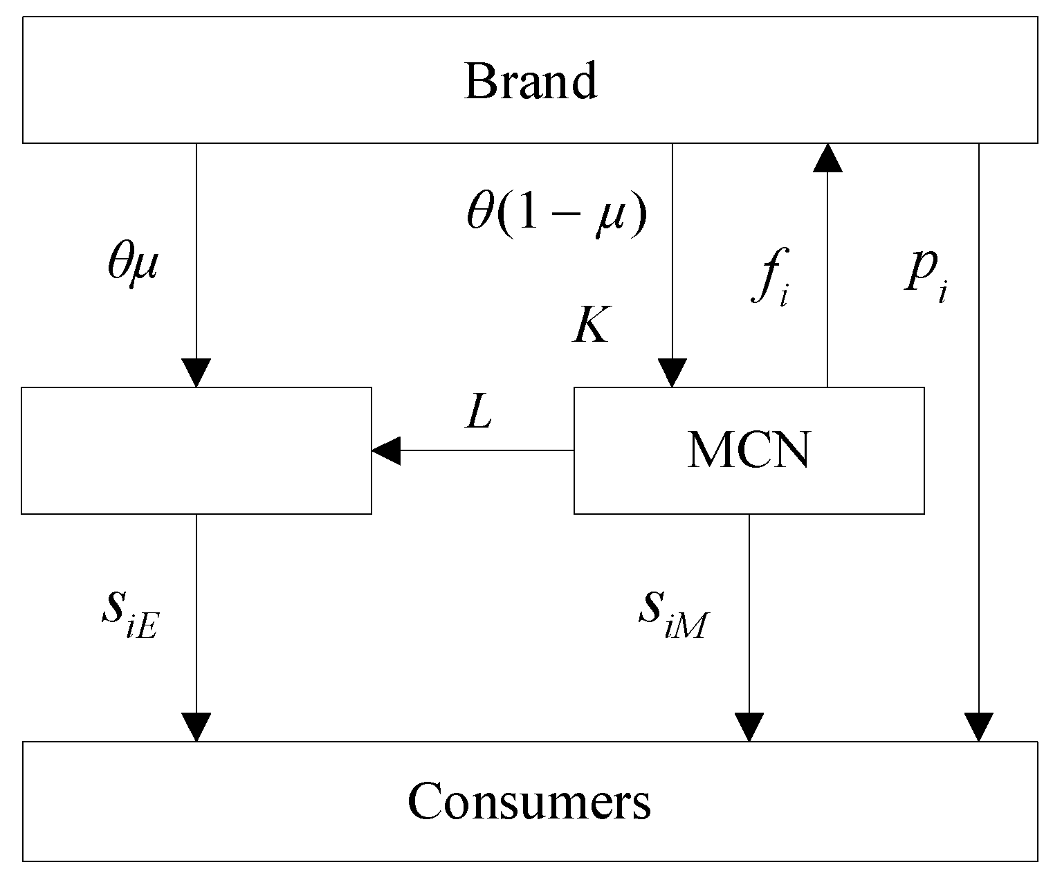
3. Problem Formulation

3.1. Subsection

Consider a market consist of one platform, one brand, and one MCN. Suppose that there are three return policies in the market, that is, the brand offers return-freight insurance (Model H), consumers purchase return-freight insurance (Model C), the brand and MCN jointly insure return-freight insurance (Model T). Let I = { H , C , T } represent the collection of return policies. We aim to study the band how to decide return policy by considering click farming from MCN and consumer disappointment aversion under live streaming e-commerce. The sales network is shown in Figure 1.
Before live streaming starts, the brand decides to pay pit fee K to MCN and total commission rate θ [ 0 , 1 ] to MCN and platform, while MCN needs to pay entry fee L to platform. After live streaming, the brand will distribute θ μ sales of the unreturned order to platform and θ ( 1 μ ) sales to MCN, where μ [ 0 , 1 ] is the sharing ratio between platform and MCN.
The decision-making sequence of live streaming e-commerce sales network is as follows: first, the brand determines the unit price p i of product under the return policy i I . Second, at the beginning of live streaming, MCN determines its service level s i M and purchases click farming volume f i (if MCN does not use click farming, then f i = 0 ), which can increase the initial sales of live stream to attract potential consumers. At the same time, the platform determines its service level s i E .
See Table 1 for descriptions of variables, parameters, and upper/lower indices involved in this paper.

3.2. Assumptions

Throughout, we make the following basic assumptions:
  • The market size is deterministic and, without loss of generality, we normalize it to 1 [31,32,39].
  • The marginal cost of the product is 0 [22].
  • The entry fee L and the pit fee K are both exogenous variables [23].
  • Every consumer represents at most a unit demand for the product [31,38].
  • All consumers are disappointment-aversion [1].

4. The Models

In this section, we apply game theory to the network to construct some leader-follower models with the brand as leader and the platform and MCN as followers under different return policies. When consumers are satisfied with the product, they will keep it. On the contrary, if they are dissatisfied with it, they will return it. It is assumed that there is heterogeneity in product valuations of consumers, which follows a uniform distribution on [ 0 , 1 ] with valuation to be 0 when consumer is dissatisfied with the product [2,31,38]. Assume that the cost of service of platform and MCN are s i E 2 2 and s i M 2 2 a respectively, where a ( 0 , 1 ] represents the ability of MCN (including operation ability and the number of fans, etc.) [23]. Since MCN will return the product purchased by click farming later and obtain a full refund, the cost of click farming is only related to click farming volume. We assume the cost of click farming to be f i 2 2 [11].

4.1. Model H for Return-Freight Insurance by Brand

Suppose that, if product is returned, return-freight insurance is only insured by the brand. First, we consider consumers’ non-psychological utility. When a consumer is satisfied with the product, his/her utility is v + α E s H E + α M s H M + ρ f H p H , where α E ,   α M represent the sensitivity coefficient of consumers to the service level of platform and MCN, respectively, and ρ represents the sensitivity coefficient of consumers to the sales volume via live stream [11]. When a consumer is dissatisfied with the product, he/she will return the product and get a full refund. Since the return freight will be paid by the insurance company, his/her utility is α E s H E + α M s H M + ρ f H . Then, the non-psychological utility of the consumer is
U H 1 = ( 1 β ) ( v + α E s H E + α M s H M + ρ f H p H ) + β ( α E s H E + α M s H M + ρ f H ) = ( 1 β ) ( v p H ) + α E s H E + α M s H M + ρ f H ,
where β represents the probability that the consumer is dissatisfied with the product.
Second, we consider consumers’ psychological utility. Bell showed in [1] that elation and disappointment are generated by comparison with previous expectations. According to Bell’s disappointment model in [1], when a consumer is satisfied with the product, he/she will feel elation. The elation coefficient is e [ 0 , 1 ] and his/her utility is
e ( ( v + α E s H E + α M s H M + ρ f H p H ) ( ( 1 β ) ( v p H ) + α E s H E + α M s H M + ρ f H ) ) = e β ( v p H ) .
when a consumer is dissatisfied with the product, the disappointment coefficient is d [ 0 , 1 ] and the utility is
d ( ( α E s H E + α M s H M + ρ f H ) ( ( 1 β ) ( v p H ) + α E s H E + α M s H M + ρ f H ) ) = d ( 1 β ) ( v p H ) .
Let ξ = d e , known as disappointment aversion level, denote the difference value between the degrees of disappointment and elation. Since the impact of disappointment on utility of disappoint-averse consumers is greater than that of elation, thus ξ > 0 [2]. By taking into account the influence of disappointment and elation, the consumer’s psychological utility is
U H 2 = e β ( 1 β ) ( v p H ) d β ( 1 β ) ( v p H ) = ξ β ( 1 β ) ( v p H ) .
The total utility of a consumer is equal to the sum of non-psychological utility and psychological utility, that is,
U H = U H 1 + U H 2 = ( 1 ξ β ) ( 1 β ) ( v p H ) + α E s H E + α M s H M + ρ f H .
Only when the consumer expected utility U H 0 , which means
v v H = p H α E s H E + α M s H M + ρ f H ( 1 ξ β ) ( 1 β ) ,
the consumer will buy the product. At this time, the sales volume of brand includes the real demand D H of consumers and the fake sales volume f H generated by click farming. Thus, the demand function is
D H = v H 1 d v = ( 1 ξ β ) ( 1 β ) ( 1 p H ) + α E s H E + α M s H M + ρ f H ( 1 ξ β ) ( 1 β ) .
The platform’s model is to decide its service level s H E by maximizing its profit, that is,
max s H E 0   π H E ( s H E ) = θ μ ( 1 β ) p H D H s H E 2 2 + L ,
where the objective consists of sales share, service cost, and entry fee. By the backward derivation method, the optimal service level of the platform is s H E *   ( p H ) = θ μ α E p H 1 ξ β . Then, MCN decides its service level s H M and click farming volume f H to maximize its profit, that is,
max s H M 0 ,   f H 0   π H M ( s H M , f H ) = θ ( 1 μ ) ( 1 β ) p H D H s H M 2 2 a f H 2 2 + K L ,
where the objective consists of sales share, service cost, click farming cost, pit fee, and entry fee. The optimal service level and the optimal click farming volume of MCN can be obtained as
s H M *   ( p H ) = a θ ( 1 μ ) α M p H 1 ξ β , f H *   ( p H ) = θ ( 1 μ ) ρ p H 1 ξ β .
The brand’s profit consists of sales, returned salvage value, return-freight insurance cost and pit fee. Since MCN will return all products purchased by click farming, no commission will be shared for this kind products f H . The product price should meet p H λ to ensure the revenue and hence the leader-follower model H for the brand is as follows:
max p H λ   π H B ( p H ) = ( ( 1 θ ) ( 1 β ) p H + β r ) D H * ( p H ) λ ( D H * ( p H ) + f H *   ( p H ) ) K ,
where r represents the unit return salvage value and λ represents the unit return-freight insurance cost. Without loss of generality, we assume that the return salvage value is greater than the return-freight insurance price, namely, r λ . In traditional e-commerce, the salvage value of returned products is generally lower than the product price [44,45,46]. However, due to the strong promotion ability of live streaming e-commerce [20], some brands are willing to conduct live streaming at a price lower than the market price to gain popularity [22], so there is a possibility that the salvage value is higher than the price. Therefore, we assume that the product price is higher than the return-freight insurance price, that is, p λ . By the way, there is no size relationship between the product price and the returned salvage value.
We can derive the following equilibrium results for Mode H.
Proposition 1.
In Model H, If β ( 0 , 1 ) ,   θ [ 0 , ( 1 ξ β ) 2 ( 1 β ) ( 2 μ ) α M 2 ] ,   λ [ 0 , ( 1 θ ) ( 1 ξ β ) ( 1 β ) ( 1 ξ β ) ( 1 + β ) + θ ] , r [ λ , ( 1 θ ) ( 1 ξ β ) ( 1 β ) ( 1 ξ β + θ ) λ ( 1 ξ β ) β ] ,   ξ [ 0 , 1 ] ,   α M [ 0 , 1 ] ,   μ [ 0 , 1 ] , then the optimal sales price for the brand, the optimal service level of the platform and MCN, and the optimal click farming volume of MCN are respectively.
p H * = ( λ β r ) G 1 ( 1 ξ β ) ( 1 β ) G 2 2 G 1 ( 1 θ ) ( 1 β ) , s H E * = θ μ α E ( ( λ β r ) G 1 ( 1 ξ β ) ( 1 β ) G 2 ) 2 G 1 ( 1 θ ) ( 1 ξ β ) ( 1 β ) , s H M * = a θ ( 1 μ ) α M ( ( λ β r ) G 1 ( 1 ξ β ) ( 1 β ) G 2 ) 2 G 1 ( 1 θ ) ( 1 ξ β ) ( 1 β ) , f H * = θ ( 1 μ ) ρ ( ( λ β r ) G 1 ( 1 ξ β ) ( 1 β ) G 2 ) 2 G 1 ( 1 θ ) ( 1 ξ β ) ( 1 β ) ,
where G 1 = ( 1 ξ β ) 2 ( 1 β ) θ ( μ α E 2 + a ( 1 μ ) α M 2 + ( 1 μ ) ρ 2 ) and G 2 = θ ( 1 μ ) ρ λ ( 1 θ ) ( 1 ξ β ) ( 1 β ) .

4.2. Model C for Return-Freight Insurance by Consumers

Suppose that return-freight insurance is insured by consumers. When a consumer is satisfied with the product, his/her utility is v + α E s C E + α M s C M + ρ f C p C λ . When he/she is dissatisfied with the product, his/her utility is α E s C E + α M s C M + ρ f C λ . Then, the non-psychological utility of the consumer is
U C 1 = ( 1 β ) ( v + α E s C E + α M s C M + ρ f C p C λ ) + β ( α E s C E + α M s C M + ρ f C λ ) = ( 1 β   ) ( v p C ) + α E s C E + α M s C M + ρ f C λ .
On the other hand, the consumer gets utility of e β ( v p C ) when he/she is satisfied with the product, and gets utility of d ( 1 β ) ( v p C ) when he/she is dissatisfied with the product. Thus, the influence of elation and disappointment on psychological utility is
U C 2 = e β ( 1 β ) ( v p C ) d β ( 1 β ) ( v p C ) = ξ β ( 1 β ) ( v p C ) .
The total utility is
U C = U C 1 + U C 2 = ( 1 ξ β ) ( 1 β ) ( v p C ) + α E s C E + α M s C M + ρ f C λ .
Only when the consumer expected utility U C 0 , which means
v v C = p C α E s C E + α M s C M + ρ f C λ ( 1 ξ β ) ( 1 β ) ,
The consumer will buy the product. In this case, the demand function is
D C = v C 1 d v = ( 1 ξ β ) ( 1 β ) ( 1 p C ) + α E s C E + α M s C M + ρ f C λ ( 1 ξ β ) ( 1 β ) .
The platform decides its service level s C E by maximizing its profit, that is,
max s C E 0   π C E ( s C E ) = θ μ ( 1 β ) p C D C   s C E 2 2 + L ,
By the backward derivation method, the optimal service level of the platform is s C E * ( p C ) = θ μ α E p C 1 ξ β . MCN sets its service level s C M and click farming volume f C by maximizing its profit, that is,
max s C M 0 ,   f C 0   π C M ( s C M , f C ) = θ ( 1 μ ) ( 1 β ) p C D C   s C M 2 2 a f C 2 2 + K L ,
The optimal service level and the optimal click farming volume of MCN can be obtained as
s C M * ( p C ) = a θ ( 1 μ ) α M p C 1 ξ β , f C * ( p C ) = θ ( 1 μ ) ρ p C 1 ξ β .
The brand’s profit consists of sales, returned salvage value, and pit fee. Then, we give a leader-follower model C for the brand as follows:
max p C 0   π C B ( p C ) = ( ( 1 θ ) ( 1 β ) p C + β r ) D C * ( p C ) K ,
We can derive the following equilibrium results for Mode C.
Proposition 2.
In Mode C, if β ( 0 , 1 ) ,   ξ [ 0 , 1 ] ,   α M [ 0 , 1 ] ,   μ [ 0 , 1 ] , θ [ 0 , ( 1 ξ β ) 2 ( 1 β ) ( 2 μ ) α M 2 ] , λ [ 0 , ( 1 θ ) ( 1 ξ β ) ( 1 β ) ( 1 ξ β ) β + 1 θ ] ,   r [ λ , ( 1 θ ) ( ( 1 ξ β ) ( 1 β ) λ ) ( 1 ξ β ) β ] , then the optimal sales price for the brand, the optimal service level of the platform and MCN, and the optimal click farming volume of MCN are respectively.
p C * = ( 1 θ ) ( 1 ξ β ) ( 1 β ) ( ( 1 ξ β ) ( 1 β ) λ ) G 1 β r 2 G 1 ( 1 θ ) ( 1 β ) , s C E * = θ μ α E ( ( 1 θ ) ( 1 ξ β ) ( 1 β ) ( ( 1 ξ β ) ( 1 β ) λ ) G 1 β r ) 2 G 1 ( 1 θ ) ( 1 ξ β ) ( 1 β )   , s C M * = a θ ( 1 μ ) α M ( ( 1 θ ) ( 1 ξ β ) ( 1 β ) ( ( 1 ξ β ) ( 1 β ) λ ) G 1 β r ) 2 G 1 ( 1 θ ) ( 1 ξ β ) ( 1 β )   , f C * = θ ( 1 μ ) ρ ( ( 1 θ ) ( 1 ξ β ) ( 1 β ) ( ( 1 ξ β ) ( 1 β ) λ ) G 1 β r ) 2 G 1 ( 1 θ ) ( 1 ξ β ) ( 1 β ) .

4.3. Model T for Return-Freight Insurance Jointly by Brand and MCN

Suppose that the return-freight insurance is jointly insured by brand and MCN. Similarly, as in Section 4.1, the demand function is
D T = v T 1 d v   = ( 1 ξ β ) ( 1 β ) ( 1 p T ) + α E s T E + α M s T M + ρ f T ( 1 ξ β ) ( 1 β ) .
The platform sets its service level s T E by maximizing its profit, that is,
max s T E 0   π T E = θ μ ( 1 β ) p T D T s T E 2 2 + L ,
By the backward derivation method, the optimal service level of the platform is s T E * ( p T ) = θ μ α E p T 1 ξ β . MCN sets its service level s T M and click farming volume f T by maximizing its profit, that is,
max s T M 0 ,   f T 0   π T M ( s T M , f T ) = θ ( 1 μ ) ( 1 β ) p T D T ( D T + f T ) ( 1 δ ) λ s T M 2 2 a f T 2 2 + K L ,
The optimal service level and the optimal click farming volume of MCN can be obtained as
s T M * ( p T ) = a α M ( θ ( 1 μ ) ( 1 β ) p T ( 1 δ ) λ ) ( 1 ξ β ) ( 1 β ) , f T * ( p T ) = θ ( 1 μ ) ( 1 β ) ρ p T ( ( 1 ξ β ) ( 1 β ) + ρ ) ( 1 δ ) λ ( 1 ξ β ) ( 1 β ) .
The brand’s profit consists of sales, returned salvage value, return-freight insurance cost and pit fee. Then, we get a leader-follower model T for the brand as follows:
max p T δ λ   π T B ( p T ) = ( ( 1 θ ) ( 1 β ) p T + β r ) D T * ( p T ) ( D T * ( p T ) + f T * ( p T ) ) δ λ K ,
We can derive the following equilibrium results for Mode T.
Proposition 3.
In Model T, if θ [ 0 , ( 1 ξ β ) 2 ( 1 β ) ( 2 μ ) α M 2 ] , β ( 0 , 1 ) , ξ [ 0 , 1 ] , α M [ 0 , 1 ] , μ [ 0 , 1 ] , ρ [ 0 , 1 ] , λ [ 0 , θ ( 1 μ ) ( 1 θ ) ( 1 β ) ρ ( 1 θ ) ( 1 δ ) ( ( 2 + ρ ) ( ( 1 ξ β ) ( 1 β ) + ρ ) + a α M 2 ) + θ ( 1 μ ) ρ β ] and r [ λ , ( 1 θ ) ( 1 β ) + δ λ β ( 1 θ ) ( 1 δ ) ( ( 2 + ρ ) ( ( 1 ξ β ) ( 1 β ) + ρ ) + a α M 2 ) λ θ ( 1 μ ) ρ β ] , then the optimal sales price for the brand, the optimal service level of the platform and MCN, and the optimal click farming volume of MCN are respectively:
p T * = ( δ λ β r ) G 1 ( 1 θ ) G 3 ( 1 ξ β ) ( 1 β ) G 4 2 G 1 ( 1 θ ) ( 1 β ) , s T E * = θ μ α E ( ( δ λ β r ) G 1 ( 1 θ ) G 3 ( 1 ξ β ) ( 1 β ) G 4 ) 2 G 1 ( 1 θ ) ( 1 ξ β ) ( 1 β ) , s T M * = a θ ( 1 μ ) α M ( ( δ λ β r ) G 1 ( 1 θ ) G 3 ( 1 ξ β ) ( 1 β ) G 4 ) 2 G 1 ( 1 θ ) ( 1 ξ β ) ( 1 β ) a α M ( 1 δ ) λ ( 1 ξ β ) ( 1 β ) , f T * = θ ( 1 μ ) ρ ( ( δ λ β r ) G 1 ( 1 θ ) G 3 ( 1 ξ β ) ( 1 β ) G 4 ) 2 G 1 ( 1 θ ) ( 1 ξ β ) ( 1 β ) ( ( 1 ξ β ) ( 1 β ) + ρ ) ( 1 δ ) λ ( 1 ξ β ) ( 1 β ) ,
where G 3 = ( a α M 2 + ( ( 1 ξ β ) ( 1 β ) + ρ ) ρ ) ( 1 δ ) λ and G 4 = θ ( 1 μ ) ρ δ λ ( 1 θ ) ( 1 ξ β ) ( 1 β ) .

5. Numerical Experiments

This section reports our numerical experiments on return policy selection and its impact on all members in the network and further gives some management enlightenments. In our experiments, we used MATLAB 9.6.0 to solve the problems involved. Recall that the three return policy models involve a total of 10 parameters, namely, consumer disappointment aversion level ξ , ability a of MCN, commission rate θ , consumer dissatisfaction β , commission sharing ratio μ between platform and MCN, unit return-freight insurance price λ , unit returned product salvage value r , consumer sensitivity α E to service level of platform, consumer sensitivity α M to service level of MCN, consumer sensitivity ρ to sales volume, brand’s return-freight insurance purchasing ratio δ (only used in Model T). The benchmark parameters were set as λ = 0.02 ,   μ = 0.2 ,   r = 0.1 ,   β = 0.4 ,   α E = 0.3 ,   α M = 0.5 ,   ρ = 0.4 ,   K = 0.08 ,   L = 0.05 .
By substituting (4), (8), (12) into (3), (7), (11) the brand’s optimal profits under three return policies are respectively:
π H B * = ( 1 ξ β ) ( 1 β ) G 2 2 ( λ β r ) ( 2 θ ( 1 μ ) ρ λ G 2 ) G 1 2 G 1 ( 1 θ ) ( 1 ξ β ) ( 1 β ) ( 1 ξ β ) 2 ( 1 β ) 2 G 2 2 ( λ β r ) 2 G 1 2 4 G 1 ( 1 θ ) ( 1 ξ β ) 2 ( 1 β ) 2 K , π C B * = ( ( 1 θ ) ( 1 ξ β ) ( 1 β ) ( ( 1 ξ β ) ( 1 β ) λ ) + G 1 β r ) 2 4 G 1 ( 1 θ ) ( 1 ξ β ) 2 ( 1 β ) 2 K , π T B * = ( ( δ λ β r ) G 1 + ( 1 θ ) G 3 ) 2 ( 1 ξ β ) 2 ( 1 β ) 2 G 4 2 4 G 1 ( 1 θ ) ( 1 ξ β ) 2 ( 1 β ) 2 + ( ( 1 ξ β ) ( 1 β ) + ρ ) ( 1 δ ) δ λ 2 ( 1 ξ β ) ( 1 β ) ( δ λ β r ) ( 2 θ ( 1 μ ) ρ δ λ G 4 ) G 1 ( ( 1 θ ) G 3 + ( 1 ξ β ) ( 1 β ) G 4 ) G 4 2 G 1 ( 1 θ ) ( 1 ξ β ) ( 1 β ) K
By substituting (4), (8), (12) into (1), (5), (9), the platform’s optimal profits under three return policies are respectively:
π H E * = θ μ ( ( 1 ξ β ) 2 ( 1 β ) 2 G 2 2 ( λ β r ) 2 G 1 2 ) 4 G 1 ( 1 θ ) 2 ( 1 ξ β ) 2 ( 1 β ) 2 θ 2 μ 2 α E 2 ( ( 1 ξ β ) ( 1 β ) G 2 ( λ β r ) G 1 ) 2 8 G 1 2 ( 1 θ ) 2 ( 1 ξ β ) 2 ( 1 β ) 2 θ μ ( ( 1 ξ β ) ( 1 β ) G 2 ( λ β r ) G 1 ) 2 G 1 ( 1 θ ) + L π C E * = θ μ ( ( 1 θ ) 2 ( 1 ξ β ) 2 ( 1 β ) 2 ( ( 1 ξ β ) ( 1 β ) λ ) 2 G 1 2 β 2 r 2 ) 4 G 1 ( 1 θ ) 2 ( 1 ξ β ) 2 ( 1 β ) 2 θ 2 μ 2 α E 2 ( ( 1 θ ) ( 1 ξ β ) ( 1 β ) ( ( 1 ξ β ) ( 1 β ) λ ) G 1 β r ) 2 8 G 1 2 ( 1 θ ) 2 ( 1 ξ β ) 2 ( 1 β ) 2 + L π T E * = θ μ ( ( δ λ β r ) G 1 ( 1 θ ) G 3 ( 1 ξ β ) ( 1 β ) G 4 ) 2 G 1 ( 1 θ ) θ μ ( ( ( δ λ β r ) G 1 ( 1 ξ β ) ( 1 β ) G 4 ) 2 ( 1 θ ) 2 G 3 2 ) 4 G 1 ( 1 θ ) 2 ( 1 ξ β ) 2 ( 1 β ) 2 θ 2 μ 2 α E 2 ( ( δ λ β r ) G 1 ( 1 θ ) G 3 ( 1 ξ β ) ( 1 β ) G 4 ) 2 8 G 1 2 ( 1 θ ) 2 ( 1 ξ β ) 2 ( 1 β ) 2 + L ,
In addition, by substituting (4), (8), (12) into (2), (6), (10), MCN’s optimal profits under three return policies are respectively:
π H M * = θ ( 1 μ ) ( ( 1 ξ β ) 2 ( 1 β ) 2 G 2 2 ( λ β r ) 2 G 1 2 ) 4 G 1 ( 1 θ ) 2 ( 1 ξ β ) 2 ( 1 β ) 2 θ 2 ( 1 μ ) 2 ( a α M 2 + ρ 2 ) ( ( 1 ξ β ) ( 1 β ) G 2 ( λ β r ) G 1 ) 2 8 G 1 2 ( 1 θ ) 2 ( 1 ξ β ) 2 ( 1 β ) 2 θ ( 1 μ ) ( ( 1 ξ β ) ( 1 β ) G 2 ( λ β r ) G 1 ) 2 G 1 ( 1 θ ) + K L π C M * = θ ( 1 μ ) ( ( 1 θ ) 2 ( 1 ξ β ) 2 ( 1 β ) 2 ( ( 1 ξ β ) ( 1 β ) λ ) 2 G 1 2 β 2 r 2 ) 4 G 1 ( 1 θ ) 2 ( 1 ξ β ) 2 ( 1 β ) 2 θ 2 ( 1 μ ) 2 ( a α M 2 + ρ 2 ) ( ( 1 θ ) ( 1 ξ β ) ( 1 β ) ( ( 1 ξ β ) ( 1 β ) λ ) G 1 β r ) 2 8 G 1 2 ( 1 θ ) 2 ( 1 ξ β ) 2 ( 1 β ) 2 + K L π T M * = θ ( 1 μ ) ( ( δ λ β r ) G 1 ( 1 θ ) G 3 ( 1 ξ β ) ( 1 β ) G 4 ) 2 G 1 ( 1 θ ) + ( 1 δ ) G 3 λ ( G 1 + θ ( 1 μ ) ρ ( 1 ξ β ) ( 1 β ) ) 2 G 1 ( 1 ξ β ) 2 ( 1 β ) 2 + ( 1 δ ) λ ( G 1 θ ( 1 μ ) ρ ( 1 ξ β ) ( 1 β ) ) ( ( δ λ β r ) G 1 ( 1 ξ β ) ( 1 β ) G 4 ) 2 G 1 ( 1 θ ) ( 1 ξ β ) 2 ( 1 β ) 2 + ( 1 δ ) 2 λ 2 ( ( 1 ξ β ) 2 ( 1 β ) 2 a α M 2 ρ 2 ) 2 ( 1 ξ β ) 2 ( 1 β ) 2 θ ( 1 μ ) G 3 2 ( 2 G 1 + θ ( 1 μ ) ( a α M 2 + ρ 2 ) ) 8 G 1 2 ( 1 ξ β ) 2 ( 1 β ) 2 + θ ( 1 μ ) G 3 ( 2 G 1 + θ ( 1 μ ) ( a α M 2 + ρ 2 ) ) ( ( δ λ β r ) G 1 ( 1 ξ β ) ( 1 β ) G 4 ) 4 G 1 2 ( 1 θ ) ( 1 ξ β ) 2 ( 1 β ) 2 θ ( 1 μ ) ( 2 G 1 + θ ( 1 μ ) ( a α M 2 + ρ 2 ) ) ( ( δ λ β r ) G 1 ( 1 ξ β ) ( 1 β ) G 4 ) 2 8 G 1 2 ( 1 θ ) 2 ( 1 ξ β ) 2 ( 1 β ) 2 ( 1 δ ) λ + K L

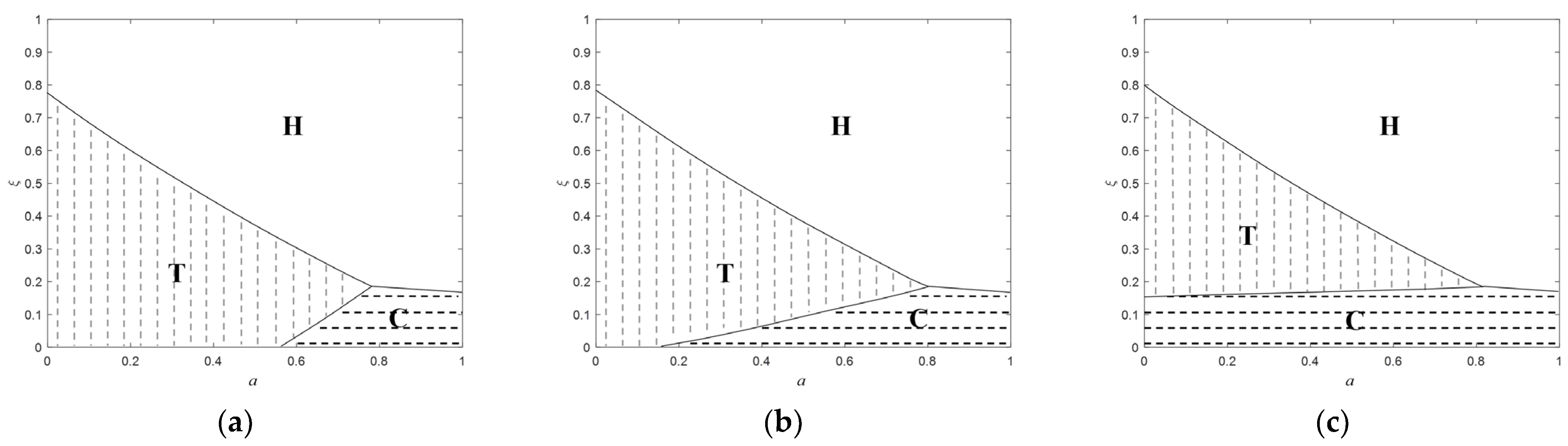
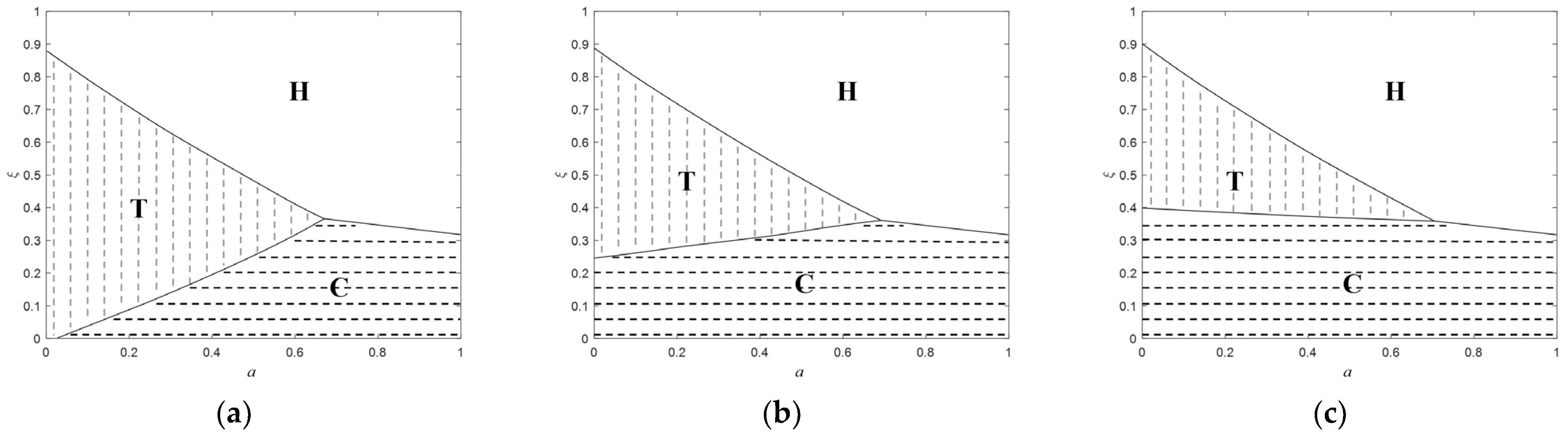
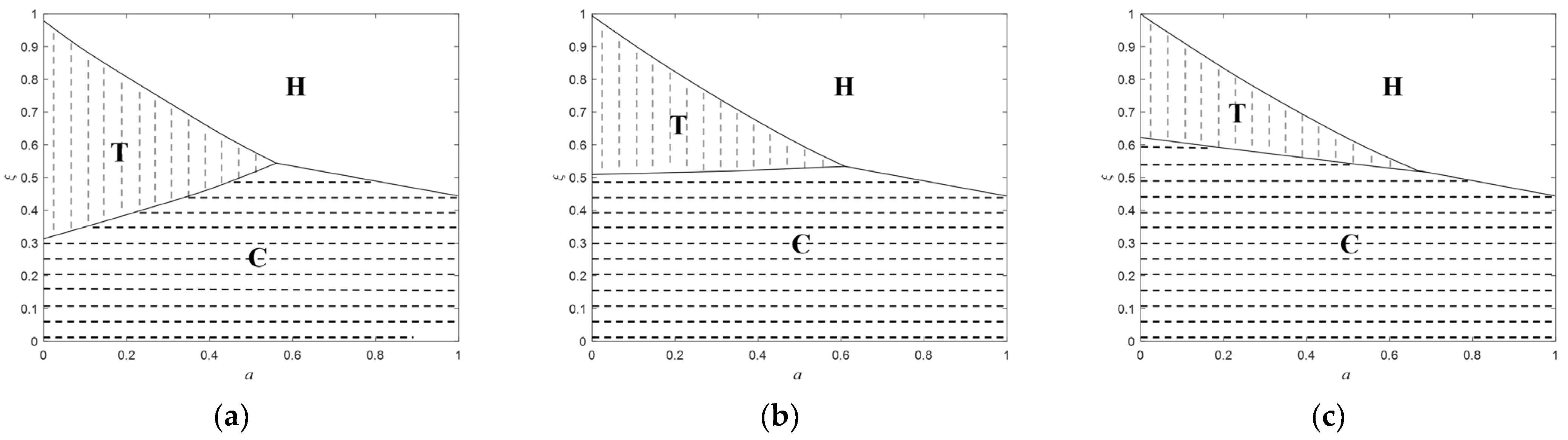
5.1. Return Policy Selection

By comparing the difference values of brand’s profits under three return policies, we analyzed the influence of consumer disappointment aversion level ξ , ability a of MCN, commission rate θ , and brand’s return-freight insurance purchasing ratio δ on brand’s return policy selection. By changing the values of θ and δ , we further investigated the influence of ξ and a on brand’s return policy selection. Referring to Proposition 1–3, we chose the parameters ξ [ 0 , 1 ] ,   a ( 0 , 1 ] ,   δ [ 0.6 , 0.9 ] . Since the commission rate θ generally does not exceed 30% [47], we discussed three cases of low commission rate ( θ = 0.1 ), medium commission rate ( θ = 0.2 ), and high commission rate ( θ = 0.3 ), respectively.

5.1.1. Low Commission Rate Scenario ( θ = 0.1 )

In our numerical experiments, different values of δ were selected to observe the influence of ξ and a on brand’s return policy selection. The result is shown in Figure 2, in which the blank region H, the horizontal line region C, and the vertical line region T represent the regions where the brand could obtain the maximum profit by choosing return policies of return-freight insurance by brand, consumers purchase return-freight insurance, and brand and MCN jointly insure return-freight insurance, respectively.
It can be seen that, in the cases of δ = 0.6 and δ = 0.75 , if a [ 0 , 0.8 ] , the brand should choose return policy H when consumers’ disappointment aversion level is high; when consumers’ disappointment aversion level is high and the ability of MCN is weak, the brand should choose return policy T; when consumers’ disappointment aversion level is low and the ability of MCN is strong, the brand should choose return policy C. If a ( 0.8 , 1 ] , when consumers’ disappointment aversion level is high, the brand should choose return policy H; otherwise, it should choose return policy C. In the case of δ = 0.9 , if a ( 0 , 0.8 ] , the brand should choose return policy H when consumers’ disappointment aversion level is high and the ability of MCN is strong; when consumers’ disappointment aversion level is high and the ability of MCN is weak, the brand should choose return policy T; when consumers’ disappointment aversion level is low, the brand should choose return policy C. If a ( 0.8 , 1 ] , it is the same as the cases of δ = 0.6 and δ = 0.75 .

5.1.2. Medium Commission Rate Scenario ( θ = 0.2 )

The numerical results for this case are shown in Figure 3. In the case of δ = 0.6 , if a ( 0 , 0.65 ] , the brand should choose return policy H when consumers’ disappointment aversion level is high; when the ability of MCN is weak, the brand should choose return policy T; when consumers’ disappointment aversion level is low and the ability of MCN is strong, the brand should choose return policy C. If a ( 0.65 , 1 ] , when consumers’ disappointment aversion level is high, the brand should choose return policy H; otherwise, it should choose return policy C. In the cases of δ = 0.75 and δ = 0.75 , if a ( 0 , 0.7 ] , the brand should choose return policy H when consumers’ disappointment aversion level is high and the ability of MCN is strong; when consumers’ disappointment aversion level is high and the ability of MCN is weak, the brand should choose return policy T; when consumers’ disappointment aversion level is low, the brand should choose return policy C. If a ( 0.7 , 1 ] , it is the same as the case of δ = 0.6 .

5.1.3. High Commission Rate Scenario ( θ = 0.3 )

The numerical results for this case are shown in Figure 4. It can be seen that, in the cases of δ = 0.6 and δ = 0.9 , if a ( 0 , 0.7 ] , the brand should choose return policy H when consumers’ disappointment aversion level is high and the ability of MCN is strong; when consumers’ disappointment aversion level is high and the ability of MCN is weak, the brand should choose return policy T; when consumers’ disappointment aversion level is low, the brand should choose return policy C. If a ( 0.7 , 1 ] , when consumers’ disappointment aversion level is high, the brand should choose return policy H; otherwise, it should choose return policy C.
According to the above analysis, when the ability of MCN is weak, the brand should choose return policy H if consumer’s disappointment aversion level is high, it should choose return policy T if consumers’ disappointment aversion level is medium, and it should choose return policy C if consumers’ disappointment aversion level is low. When the ability of MCN is strong, the brand should choose return policy H if consumers’ disappointment aversion level is high and, otherwise, it should choose return policy C. This indicates that return policy T is not applicable when the ability of MCN is strong. The reason may be because MCN has more bargaining power in this case and the brand is less likely to reduce costs by making MCN bear enough purchasing cost of freight insurance. We also note that return policy C is more applicable when consumers have low disappointment aversion level. This may be because the disappointment has a small impact on consumers’ utility, in other words, consumers are less sensitive to possible loss caused by the return. In this case, the brand can choose to entice consumers to buy return-freight insurance by themselves instead of offering them freight insurance for free.
In addition, combining with Figure 2, Figure 3 and Figure 4, it can be found that, with the increase of brand’s return-freight insurance purchasing ratio, region C increases significantly, region T decreases significantly, while region H does not change significantly. This reveals that brand’s return-freight insurance purchasing ratio has a great influence on whether the brand chooses return policy C or T, but has almost no influence on whether the brand chooses return policy H. In comparison, with the increase of commission rate, regions H and T significantly decreases, while region C significantly increases. This indicates that return policies H and T are more suitable for use with low commission rate, while return policy C is more suitable for use with high commission rate.
To sum up, return policy H is more suitable for brands to sell products with low commission rate or with high consumer disappointment aversion level. Compared with return policy H, return policy T is more suitable for brands who can bear low return-freight insurance purchasing ratio or collaborate with MCN with low ability, which requires brands with high leadership and strong bargaining power, so that MCN is willing to bear more return-freight insurance purchase cost. This suggests that return policy T is a better choice when high leadership brands partner with waist or tail MCN. Compared with previous two return strategies, return policy C is more suitable for brands to sell products with high commission rate or with low consumer disappointment aversion level. Moreover, return policy C is a better choice than return policy T when return-freight insurance purchasing ratio for brands is relatively high. This indicates that, when brands’ leadership is low, return policy C may obtain high profits.

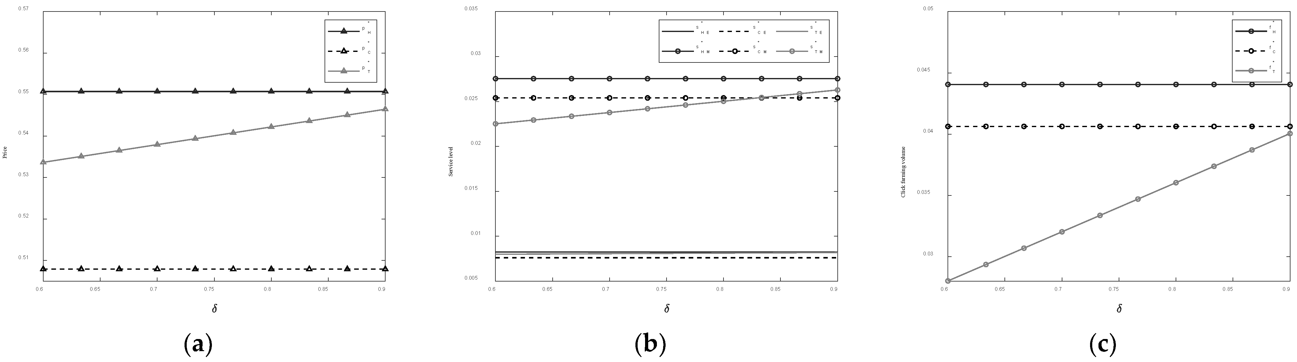
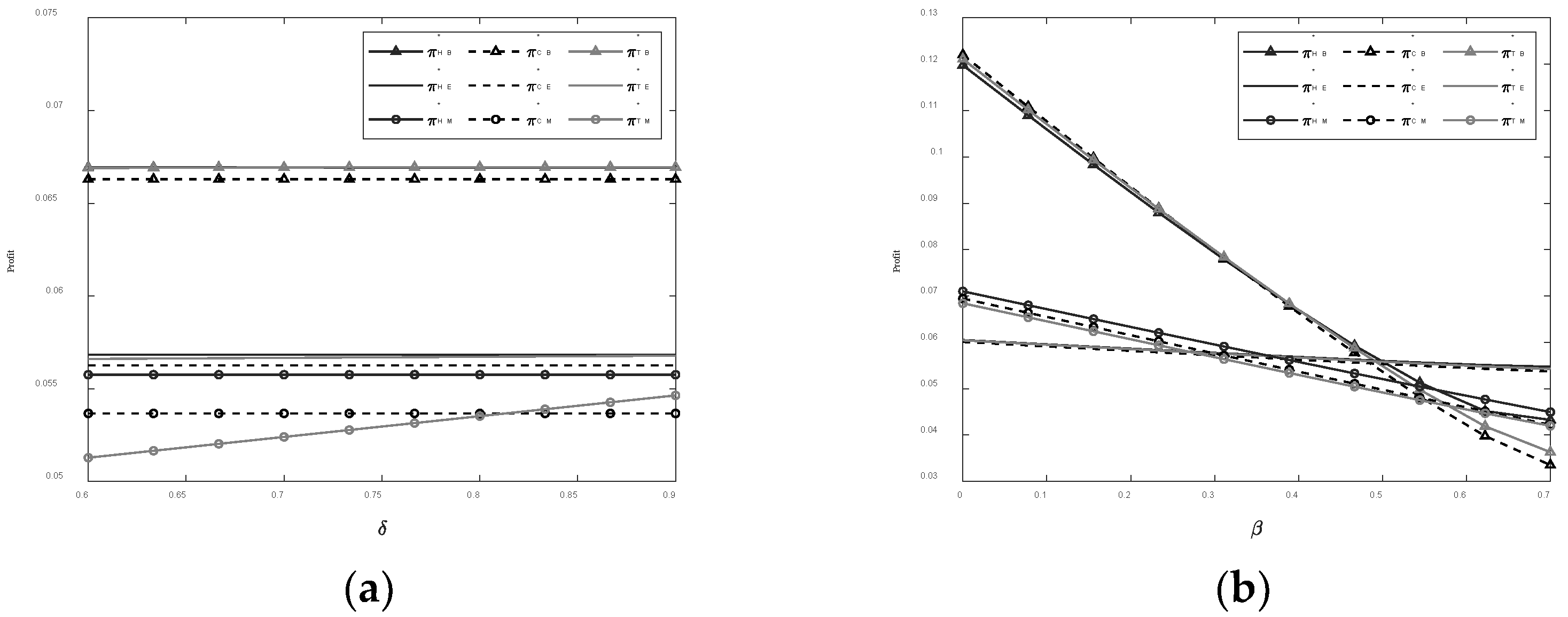
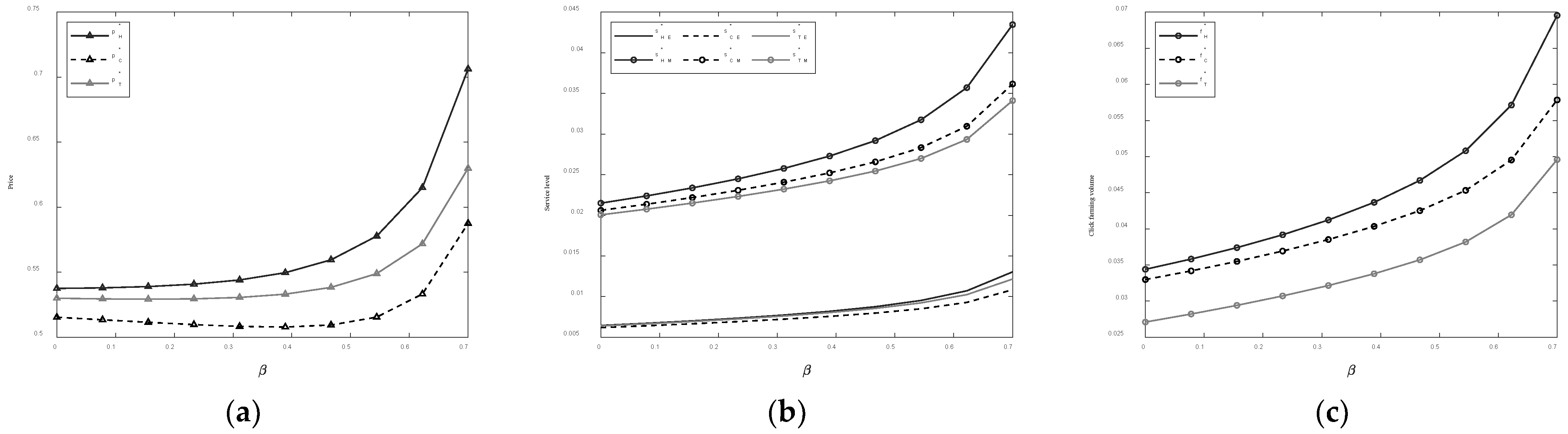
5.2. Sensitivity Analysis of Optimal Decisions

Five important parameters are involved in this section, which are consumer disappointment aversion level ξ , ability a of MCN, brand’s return-freight insurance purchasing ratio δ , commission rate θ , and consumer dissatisfaction β . We made some numerical experiments to analyze the influence of these parameters on each member in the system. The benchmark parameters were respectively taken as ξ = 0.5 ,   a = 0.5 ,   δ = 0.75 ,   θ = 0.2 .
The experimental results related to the influence of consumer disappointment aversion level ξ [ 0 , 1 ] , ability of MCN a ( 0 , 1 ] , and commission rate θ [ 0 , 0.3 ] on each member are shown in Figure 5. In particular, Figure 5a–c, Figure 5d–f, Figure 5g–i, and Figure 5j–l show the trends of optimal price, service level, click farming volume, and optimal profit of each member with the increase of ξ , a , and θ , respectively.
From Figure 5a–i, we can observe that under three return policies, optimal product price, service level, and click farming volume rise with the increase of disappointment aversion level, ability of MCN, and commission rate. This shows that, when brands sell products with high level of consumer disappointment aversion and cooperate with MCN with high ability and platform with high commission rate, the higher the product price is set to be, the higher the service levels are provided to be and the greater the amount of click farming is.
The trends of brand’s profit curve in Figure 5j,h correspond to Figure 3b, while the trend of brand’s profit curve in Figure 5l corresponds to Figure 2b, Figure 3b and Figure 4b. It can be seen from these figures that, only when consumer disappointment aversion level and MCN’s ability are both high or commission rate is low, the brand should choose return policy H, which is consistent with the conclusions in Section 5.1. Moreover, only when the brand chooses return policy H, both platform and MCN can get the maximum profits. Therefore, the whole system can be coordinated only when the brand cooperates with MCN with strong ability and sells with high consumer disappointment aversion level or with low commission rate. In other cases, because the brand does not choose return policy H, it is disadvantageous to both platform and MCN. In addition, with the increase of disappointment aversion level and the ability of MCN, the optimal profit of each member under three return policies increases, but the changes of optimal profits of platform and MCN are not significant. However, with the increase of commission rate, the optimal profit of the brand decreases, while the optimal profits of both platform and MCN increase significantly. This shows that commission rate is the main factor affecting the optimal profits of platform and MCN.
The experimental results related to the influence of return-freight insurance purchasing ratio δ [ 0.6 , 0.9 ] on each member are shown in Figure 6 and Figure 7a. From Figure 6a–c, it can be seen that p T * ,   s T M * ,   f T * rise with the increase of brand’s return-freight insurance purchasing ratio. This indicates that, under return policy T, the higher brand’s return-freight insurance purchasing ratio is, the higher the values of product price, service level provided by MCN, and click farming volume from MCN are.
The trend of brand’s profit curve in Figure 7a corresponds to Figure 3a–c. It can be seen that under the condition of ξ = 0.5 ,   a = 0.5 ,   θ = 0.2 , when brand’s return-freight insurance purchasing ratio is low, the brand should choose return policy H; otherwise, it should choose return policy T. Only when the brand chooses return policy H, the platform and MCN can get the maximal profits. Therefore, the whole system can realize the coordination only when brand’s return-freight insurance purchasing ratio is relatively low.
The experimental results related to the influence of consumer dissatisfaction on each member are shown in Figure 7b and Figure 8. According to Figure 8a, both p H * and p C * go up with the increase of consumer dissatisfaction with a trend of decreasing first and increasing later. From Figure 8b,c, it can be seen that the maximal service level and the optimal volume of click farming under three return policies rise with the increase of consumer dissatisfaction. From Figure 7b, it can be seen that, in the case of ξ = 0.5 ,   a = 0.5 ,   θ = 0.2 , when consumers are less satisfied, the brand should choose return policy C; otherwise, it should choose return policy H. Only when the brand chooses return policy H, the platform and MCN can get the maximal profits. Therefore, the whole system can be coordinated only when consumers are highly dissatisfied.
Based on the above analysis, no matter how the parameters of consumer disappointment aversion level, ability of MCN, commission rate, brand’s return-freight insurance purchasing ratio, and consumer dissatisfaction change, the brand’s optimal prices under three return policies always satisfy p H * > p T * > p C * . This is because, when a brand needs to buy return-freight insurance, it will transfer part of the purchase cost to product price. Accordingly, the optimal service levels of platform and MCN under three return policies always satisfy s H E * > s T E * > s C E * , s H M * > s C M * > s T M * and, in most cases, the service level provided by MCN is greater than that provided by the platform. The optimal click farming volumes of MCN under three return policies always satisfy f H * > f C * > f T * and f T * is significantly lower than f H * and f C * , which indicates that return policy T can effectively suppress click farming of MCN. Furthermore, when consumer disappointment aversion level, MCN’s ability, consumer dissatisfaction are all high or commission rate, brand’s return-freight insurance purchasing ratio are both low, the whole system can achieve coordination. In other cases, the optimal return policies of brand are not conducive to platform and MCN.

6. Conclusions

In the previous sections, we have taken consumer disappointment aversion and MCN click farming into account to establish leader-follower models for brand’s return policy selection under three cases of return-freight insurance by brands or by consumers or by brands and MCN jointly. In order to obtain the optimal solutions, convexity conditions of both upper and lower models were discussed, and based on these conditions, the optimal decisions of each member were given. Furthermore, numerical experiments were conducted to analyze the effects of consumer disappointment aversion level, ability of MCN, commission rate, return-freight insurance purchasing ratio, and consumer dissatisfaction on brand’s return policy selection, optimal decision, and optimal profit of each member in the network. From the above analysis, we obtained the following management enlightenments:
(i) When MCN has a weak ability, brands should choose return policy H if consumer disappointment aversion level is high, choose return policy T if consumer disappointment aversion level is medium, and choose return policy C if consumer disappointment aversion level is low. When MCN has a strong ability, brands should choose return policy H if consumer disappointment aversion level is high and choose return policy C otherwise.
(ii) Brand’s return-freight insurance purchasing ratio has a great influence on brands’ choice between return policy C and T, but almost no influence on return policy H. Moreover, return policies H and T are more suitable for platforms with low commission rate, while return policy C is more suitable for platforms with high commission rate.
(iii) The amount of MCN click farming under return policy T is significantly lower than that of other two return strategies and hence it can effectively suppress click farming behavior of MCN.
(iv) The whole system can realize coordination only when the values of consumer disappointment aversion level, ability of MCN, consumer dissatisfaction are all high or the values of commission rate, brand’s return-freight insurance purchasing ratio are all low. In other cases, brands’ return policy selection is not conducive to platforms and MCN.
In our analysis, we only considered the case with a single brand, a single platform, and a single MCN. We leave the multiple cases as a future work. For extensions from single case to multiple cases, the number of parameters will increase greatly, which will bring some difficulties in numerical analysis. How to solve these difficulties will be our next research topic.

Author Contributions

Conceptualization, G.L., W.X., Y.L. and X.Z.; methodology, W.X.; software, W.X.; validation, W.X., G.L., Y.L. and X.Z.; formal analysis, W.X. and Y.L.; investigation, W.X.; resources, Y.L.; data curation, W.X.; writing—original draft preparation, W.X.; writing—review and editing, G.L. and Y.L.; visualization, Y.L.; supervision, G.L. and Y.L.; project administration, G.L.; funding acquisition, G.L. and X.Z. All authors have read and agreed to the published version of the manuscript.

Funding

This work was supported in part by National Natural Science Foundation of China (Nos. 11901380; 12071280).

Institutional Review Board Statement

Not applicable.

Informed Consent Statement

Not applicable.

Data Availability Statement

Not applicable.

Conflicts of Interest

The authors declare no conflict of interest.

Appendix A

Proof of Proposition 1.
By substituting s H E *   ( p H ) ,   s H M * ( p H ) ,   f H * ( p H ) into the brand’s optimization problem, the single-level optimization problem becomes
max p H λ   π H B * = ( ( 1 ξ β ) 2 ( 1 β ) ( 1 p H ) + θ ( μ α E 2 + a ( 1 μ ) α M 2 + ( 1 μ ) ρ 2 ) p H ) ( ( 1 β ) ( 1 θ ) p H + β r λ ) ( 1 ξ β ) 2 ( 1 β ) θ ( 1 μ ) ρ λ p H 1 ξ β K .
Consider π H B ( p H ) = 2 ( 1 θ ) ( θ ( μ α E 2 + a ( 1 μ ) α M 2 + ( 1 μ ) ρ 2 ) ( 1 ξ β ) 2 ( 1 β ) ) ( 1 ξ β ) 2 . If β ( 0 , 1 ) , ξ [ 0 , 1 ] , α M [ 0 , 1 ] , μ [ 0 , 1 ] ,   θ [ 0 , ( 1 ξ β ) 2 ( 1 β ) ( 2 μ ) α M 2 ] , we have π H B ( p H ) < 0 , which means that π H B is concave with respect to p H . By solving π H B ( p H ) = 0 , we have p H * = ( λ β r ) G 1 ( 1 ξ β ) ( 1 β ) G 2 2 G 1 ( 1 θ ) ( 1 β ) . To ensure the constraint p H λ , it is sufficient to satisfy λ [ 0 , ( 1 θ ) ( 1 ξ β ) ( 1 β ) ( 1 ξ β ) ( 1 + β ) + θ ] and r [ λ , ( 1 θ ) ( 1 ξ β ) ( 1 β ) ( 1 ξ β + θ ) λ ( 1 ξ β ) β ] .
By substituting p H * into s H E *   ( p H ) ,   s H M * ( p H ) ,   f H * ( p H ) , we have
s H E * = θ μ α E ( ( λ β r ) G 1 ( 1 ξ β ) ( 1 β ) G 2 ) 2 G 1 ( 1 θ ) ( 1 ξ β ) ( 1 β ) , s H M * = a θ ( 1 μ ) α M ( ( λ β r ) G 1 ( 1 ξ β ) ( 1 β ) G 2 ) 2 G 1 ( 1 θ ) ( 1 ξ β ) ( 1 β ) , f H * = θ ( 1 μ ) ρ ( ( λ β r ) G 1 ( 1 ξ β ) ( 1 β ) G 2 ) 2 G 1 ( 1 θ ) ( 1 ξ β ) ( 1 β ) .
This completes the proof. □
Proof of Proposition 2.
By substituting s C E *   ( p C ) ,   s C M * ( p C ) ,   f C * ( p C ) into the brand’s optimization problem, the single-level optimization problem becomes
max p C 0   π C B * = ( ( 1 ξ β ) ( ( 1 ξ β ) ( 1 β ) ( 1 p C ) λ ) + θ ( μ α E 2 + a ( 1 μ ) α M 2 + ( 1 μ ) ρ 2 ) p C ) ( ( 1 β ) ( 1 θ ) p C + β r ) ( 1 ξ β ) 2 ( 1 β ) K .
Consider π C B ( p C ) = 2 ( 1 θ ) ( θ ( μ α E 2 + a ( 1 μ ) α M 2 + ( 1 μ ) ρ 2 ) ( 1 ξ β ) 2 ( 1 β ) ) ( 1 ξ β ) 2 . If β ( 0 , 1 ) , ξ [ 0 , 1 ] , α M [ 0 , 1 ] , μ [ 0 , 1 ] ,   θ [ 0 , ( 1 ξ β ) 2 ( 1 β ) ( 2 μ ) α M 2 ] , we have π C B ( p C ) < 0 , which means that π C B is concave with respect to p C . By solving π C B ( p C ) = 0 , we have p C * = ( 1 θ ) ( 1 ξ β ) ( 1 β ) ( ( 1 ξ β ) ( 1 β ) λ ) G 1 β r 2 G 1 ( 1 θ ) ( 1 β ) . To ensure the constraint p C 0 , it is enough to satisfy λ [ 0 , ( 1 θ ) ( 1 ξ β ) ( 1 β ) ( 1 ξ β ) β + 1 θ ] and r [ λ , ( 1 θ ) ( ( 1 ξ β ) ( 1 β ) λ ) ( 1 ξ β ) β ] .
By substituting p C * into s C E *   ( p C ) ,   s C M * ( p C ) ,   f C * ( p C ) , we have
s C E * = θ μ α E ( ( 1 θ ) ( 1 ξ β ) ( 1 β ) ( ( 1 ξ β ) ( 1 β ) λ ) G 1 β r ) 2 G 1 ( 1 θ ) ( 1 ξ β ) ( 1 β )   , s C M * = a θ ( 1 μ ) α M ( ( 1 θ ) ( 1 ξ β ) ( 1 β ) ( ( 1 ξ β ) ( 1 β ) λ ) G 1 β r ) 2 G 1 ( 1 θ ) ( 1 ξ β ) ( 1 β ) , f C * = θ ( 1 μ ) ρ ( ( 1 θ ) ( 1 ξ β ) ( 1 β ) ( ( 1 ξ β ) ( 1 β ) λ ) G 1 β r ) 2 G 1 ( 1 θ ) ( 1 ξ β ) ( 1 β ) .
This completes the proof. □
Proof of Proposition 3.
By substituting s T E *   ( p T ) ,   s T M * ( p T ) ,   f T * ( p T ) into the brand’s optimization problem, the single-level optimization problem becomes
max p T δ λ   π T B * = ( ( 1 ξ β ) 2 ( 1 β ) 2 ( 1 p T ) + θ ( 1 β ) ( μ α E 2 + a ( 1 μ ) α M 2 + ( 1 μ ) ρ 2 ) p T G 3 ) ( ( 1 β ) ( 1 θ ) p T + β r δ λ ) ( 1 ξ β ) 2 ( 1 β ) 2 ( θ ( 1 μ ) ( 1 β ) ρ p T ( ( 1 ξ β ) ( 1 β ) + ρ ) ( 1 δ ) λ ) δ λ ( 1 ξ β ) ( 1 β ) K ,
Consider π T B ( p T ) = 2 ( 1 θ ) ( θ ( μ α E 2 + a ( 1 μ ) α M 2 + ( 1 μ ) ρ 2 ) ( 1 ξ β ) 2 ( 1 β ) ) ( 1 ξ β ) 2 . If β ( 0 , 1 ) , ξ [ 0 , 1 ] , α M [ 0 , 1 ] , μ [ 0 , 1 ] ,   θ [ 0 , ( 1 ξ β ) 2 ( 1 β ) ( 2 μ ) α M 2 ] , we have π T B ( p T ) < 0 , which means that π H B is concave with respect to p T . By solving π T B ( p T ) = 0 , we have p T * = ( δ λ β r ) G 1 ( 1 θ ) G 3 ( 1 ξ β ) ( 1 β ) G 4 2 G 1 ( 1 θ ) ( 1 β ) . To ensure the constraint p T max { δ λ , ( ( 1 ξ β ) ( 1 β ) + ρ ) ( 1 δ ) λ θ ( 1 μ ) ( 1 β ) ρ } , it is sufficient to satisfy
λ [ 0 , θ ( 1 μ ) ( 1 θ ) ( 1 β ) ρ ( 1 θ ) ( 1 δ ) ( ( 2 + ρ ) ( ( 1 ξ β ) ( 1 β ) + ρ ) + a α M 2 ) + θ ( 1 μ ) ρ β ] , r [ λ , ( 1 θ ) ( 1 β ) + δ λ β ( 1 θ ) ( 1 δ ) ( ( 2 + ρ ) ( ( 1 ξ β ) ( 1 β ) + ρ ) + a α M 2 ) λ θ ( 1 μ ) ρ β ] .
By substituting p T * into s T E *   ( p T ) ,   s T M * ( p T ) ,   f T * ( p T ) , we have
s T E * = θ μ α E ( ( δ λ β r ) G 1 ( 1 θ ) G 3 ( 1 ξ β ) ( 1 β ) G 4 ) 2 G 1 ( 1 θ ) ( 1 ξ β ) ( 1 β ) , s T M * = a θ ( 1 μ ) α M ( ( δ λ β r ) G 1 ( 1 θ ) G 3 ( 1 ξ β ) ( 1 β ) G 4 ) 2 G 1 ( 1 θ ) ( 1 ξ β ) ( 1 β ) a α M ( 1 δ ) λ ( 1 ξ β ) ( 1 β ) , f T * = θ ( 1 μ ) ρ ( ( δ λ β r ) G 1 ( 1 θ ) G 3 ( 1 ξ β ) ( 1 β ) G 4 ) 2 G 1 ( 1 θ ) ( 1 ξ β ) ( 1 β ) ( ( 1 ξ β ) ( 1 β ) + ρ ) ( 1 δ ) λ ( 1 ξ β ) ( 1 β ) .
This completes the proof. □

References

  1. Bell, D.E. Disappointment in decision making under uncertainty. Oper. Res. 1985, 33, 1–27. [Google Scholar] [CrossRef]
  2. Chen, S.J.; Guan, Z.Z. Research on return policies of omni-channel retailer considering consumers disappointment aversion. China J. Manag. Sci. 2021. [Google Scholar] [CrossRef]
  3. Du, S.F.; Li, W.; Li, H. Omnichannel management with consumer disappointment aversion. Int. J. Prod. Econ. 2019, 215, 84–101. [Google Scholar] [CrossRef]
  4. Wongkitrungrueng, A.; Dehouche, N.; Assarut, A. Live streaming commerce from the sellers’ perspective: Implications for online relationship marketing. J. Market. Manag. 2020, 36, 488–518. [Google Scholar] [CrossRef]
  5. Lu, B.J.; Chen, Z.J. Live streaming commerce and consumers’ purchase intention: An uncertainty reduction perspective. Inf. Manag. 2021, 58, 103509. [Google Scholar] [CrossRef]
  6. Li, Y.; Li, X.L.; Cai, J.L. How attachment affects user stickiness on live streaming platforms: A socio-technical approach perspective. J. Retail. Consum. Serv. 2021, 60, 102478. [Google Scholar] [CrossRef]
  7. Iimedia Research. China’s Live Streaming E-Commerce Industry: The Total Scale is Expected to Reach 2137.3 Billion Yuan by 2025. 2022. Available online: https://mp.weixin.qq.com/s/kauGkdsQ8qDq4r_MA4GJZA (accessed on 3 July 2022).
  8. Zhang, P.P. Internet celebrity “Factory”: The development history, rise logic and future trend of MCN. Future Commun. 2021, 28, 48–54. [Google Scholar] [CrossRef]
  9. Huang, M.; Chu, X.P. The Problem and Governance of Internet Traffic in Live Streaming E-Commerce. 2021. Available online: https://d.wanfangdata.com.cn/periodical/ChlQZXJpb2RpY2FsQ0hJTmV3UzIwMjIwOTAxEgx4d2MyMDIxMDEwMDQaCGR5d2ZhN21t (accessed on 25 February 2021).
  10. Jiang, C.X.; Zhu, J.; Xu, Q.F. Dissecting click farming on the Taobao platform in China via PU learning and weighted logistic regression. Electron. Commer. Res. 2020, 22, 157–176. [Google Scholar] [CrossRef]
  11. Bao, L.J.; Zhong, W.J.; Mei, Z.E. The influence of “Click farming” on the sellers’ competition in e-commerce platform. Syst. Eng. Theory Pract. 2021, 41, 2876–2886. [Google Scholar]
  12. 36 Kr Research Institute. 2020 China Live Streaming E-Commerce Industry Research Report. 2020. Available online: https://36kr.com/p/986332005917833 (accessed on 2 December 2020).
  13. Fan, Z.P.; Chen, Z.W. When should the e-tailer offer complimentary return-freight insurance? Int. J. Prod. Econ. 2020, 230, 107890. [Google Scholar] [CrossRef]
  14. Ang, T.; Wei, S.; Anaza, N.A. Livestreaming vs. pre-recorded: How social viewing strategies impact consumers’ viewing experiences and behavioral intentions. Eur. J. Market. 2018, 52, 2075–2104. [Google Scholar] [CrossRef]
  15. Hou, F.F.; Guan, Z.Z.; Li, B.Y.; Chong, A.Y.L. Factors influencing people’s continuous watching intention and consumption intention in live streaming: Evidence from China. Internet Res. 2020, 1, 141–163. [Google Scholar] [CrossRef]
  16. Ma, Y.Y. To shop or not: Understanding Chinese consumers’ live-stream shopping intentions from the perspectives of uses and gratifications, perceived network size, perceptions of digital celebrities, and shopping orientations. Telemat. Inform. 2021, 59, 101562. [Google Scholar] [CrossRef]
  17. Sun, Y.; Shao, X.; Li, X.T.; Guo, Y.; Nie, K. How live streaming influences purchase intentions in social commerce: An IT affordance perspective. Electron. Commer. Res. Appl. 2019, 37, 100886. [Google Scholar] [CrossRef]
  18. Xu, X.Y.; Wu, J.H.; Li, Q. What drives consumer shopping behavior in live streaming commerce? J. Electron. Commer. Res. 2020, 21, 144–167. Available online: http://www.jecr.org/node/609 (accessed on 1 August 2020).
  19. Zhang, M.; Sun, L.; Qin, F.; Wang, G.A. E-service quality on live streaming platforms: Swift guanxi perspective. J. Serv. Mark. 2021, 35, 312–324. [Google Scholar] [CrossRef]
  20. Wang, X.; Tao, Z.Y.; Liang, L.; Gou, Q.L. An analysis of salary mechanisms in the sharing economy: The interaction between streamers and unions. Int. J. Prod. Econ. 2019, 214, 106–124. [Google Scholar] [CrossRef]
  21. Xing, P.; You, H.Y.; Fan, Y.C. Optimal quality effort strategy in service supply chain of live streaming e-commerce based on platform marketing effort. Control Decis. 2022, 37, 205–212. [Google Scholar]
  22. Hu, J.; Li, L.; Zhang, H.; Zhu, X.Z.; Yang, W.S. Dynamic pricing strategies for live broadcast platform considering reference effect and anchor influence. Syst. Eng. Theory Pract. 2022, 42, 756–766. [Google Scholar]
  23. Liu, H.Y.; Liu, S.L. Optimal decisions and coordination of live streaming selling under revenue-sharing contracts. Manag. Decis. Econ. 2021, 42, 1022–1036. [Google Scholar] [CrossRef]
  24. Zhao, J.; Lau, R.Y.K.; Zhang, W.P.; Zhang, K.H.; Chen, X.; Tang, D. Extracting and reasoning about implicit behavioral evidences for detecting fraudulent online transactions in e-commerce. Decis. Support Syst. 2016, 86, 109–121. [Google Scholar] [CrossRef]
  25. Li, N.; Du, S.G.; Zheng, H.Z.; Xue, M.H.; Zhu, H.J. Fake reviews tell no tales? Dissecting click farming in content-generated social networks. China Commun. 2018, 15, 98–109. [Google Scholar] [CrossRef]
  26. Jiang, C.X.; Zhu, J.; Xu, Q.F. Which goods are most likely to be subject to click farming? An evidence from the Taobao platform. Electron. Commer. Res. Appl. 2021, 50, 101107. [Google Scholar] [CrossRef]
  27. Fang, X.L. The control of “False transaction and credit standing” behavior in the network trading platform from the perspective of evolutionary game. Inf. Sci. 2018, 36, 89–92. [Google Scholar] [CrossRef]
  28. McWilliams, B. Money-back guarantees: Helping the low-quality retailer. Manag. Sci. 2012, 58, 1521–1524. [Google Scholar] [CrossRef]
  29. Xu, L.; Li, Y.J.; Govindan, K.; Xu, X.L. Consumer returns policies with endogenous deadline and supply chain coordination. Eur. J. Oper. Res. 2015, 242, 88–99. [Google Scholar] [CrossRef]
  30. Ren, M.; Liu, J.Q.; Feng, S.; Yang, A.F. Pricing and return strategy of online retailers based on return insurance. J. Retail. Consum. Serv. 2021, 59, 102350. [Google Scholar] [CrossRef]
  31. Chen, Z.W.; Fan, Z.P.; Zhao, X. Offering return-freight insurance or not: Strategic analysis of an e-seller’s decisions. Omega-Int. J. Manag. Sci. 2021, 103, 102447. [Google Scholar] [CrossRef]
  32. Chen, B.T.; Chen, J. When to introduce an online channel, and offer money back guarantees and personalized pricing? Eur. J. Oper. Res. 2017, 257, 614–624. [Google Scholar] [CrossRef]
  33. Radhi, M.; Zhang, G.Q. Optimal cross-channel return policy in dual-channel retailing systems. Int. J. Prod. Econ. 2019, 210, 184–198. [Google Scholar] [CrossRef]
  34. Jin, D.; Caliskan-Demirag, O.; Chen, F.; Huang, M. Omnichannel retailers’ return policy strategies in the presence of competition. Int. J. Prod. Econ. 2020, 225, 107595. [Google Scholar] [CrossRef]
  35. Loomes, G.; Sugden, R. Disappointment and dynamic consistency in choice under uncertainty. Rev. Econ. Stud. 1986, 53, 271–282. [Google Scholar] [CrossRef]
  36. Delquie, P.; Cillo, A. Expectations, disappointment, and rank-dependent probability weighting. Theory Decis. 2006, 60, 193–206. [Google Scholar] [CrossRef]
  37. Koszegi, B.; Rabin, M. Reference dependent risk attitudes. Am. Econ. Rev. 2007, 97, 1047–1073. [Google Scholar] [CrossRef] [Green Version]
  38. Liu, Q.; Shum, S. Pricing and capacity rationing with customer disappointment aversion. Prod. Oper. Manag. 2013, 22, 1269–1286. [Google Scholar] [CrossRef]
  39. Zhang, Y.; Zhang, J.L. Strategic customer behavior with disappointment aversion customers and two alleviation policies. Int. J. Prod. Econ. 2017, 191, 170–177. [Google Scholar] [CrossRef]
  40. Wang, H.; Guan, Z.Z.; Dong, D.Y.; Zhao, N. Optimal pricing strategy with disappointment-aversion and elation-seeking consumers: Compared to price commitment. Int. Trans. Oper. Res. 2021, 28, 2810–2840. [Google Scholar] [CrossRef]
  41. Simon, A.H. Models of Bounded Rationality; The MIT Press: Cambridge, MA, USA, 1982; Volume 2. [Google Scholar]
  42. Cao, B.B.; Fan, Z.P.; You, T.H. The newsvendor problem with reference dependence, disappointment aversion and elation seeking. Chaos Solitons Fractals 2017, 104, 568–574. [Google Scholar] [CrossRef]
  43. Cao, B.B.; Fan, Z.P. Ordering and sales effort investment for temperature-sensitive products considering retailer’s disappointment aversion and elation seeking. Int. J. Prod. Res. 2018, 56, 2411–2436. [Google Scholar] [CrossRef]
  44. Rintamäki, T.; Kanto, A.; Kuusela, H.; Spence, M.T. Decomposing the value of department store shopping into utilitarian, hedonic and social dimensions: Evidence from Finland. Int. J. Retail Distrib. Manag. 2006, 34, 6–24. [Google Scholar] [CrossRef]
  45. Chen, J.; Bell, P. The impact of customer returns on decisions in a newsvendor problem with and without buyback policies. Int. Trans. Oper. Res. 2011, 18, 473–491. [Google Scholar] [CrossRef]
  46. Letizia, P.; Pourakbar, M.; Harrison, T. The impact of consumer returns on the multichannel sales strategies of manufacturers. Prod. Oper. Manag. 2017, 27, 323–349. [Google Scholar] [CrossRef]
  47. Wang, Y.Y.; Yu, Z.Q. Research on the dominant models and commission coordination mechanism of e-supply chain based on e-commerce sales platform. China J. Manag. Sci. 2019, 27, 109–118. [Google Scholar]
Figure 1. Illustration of live streaming e-commerce structure.
Jtaer 17 00078 g001
Figure 2. Return policy selection of brand under low commission rate. (a) δ = 0.6 ; (b) δ = 0.75 ; (c) δ = 0.9 .
Jtaer 17 00078 g002
Figure 3. Return policy selection of brand under medium commission rate. (a) δ = 0.6 ; (b) δ = 0.75 ; (c) δ = 0.9 .
Jtaer 17 00078 g003
Figure 4. Return policy selection of brand under high commission rate. (a) δ = 0.6 ; (b) δ = 0.75 ; (c) δ = 0.9 .
Jtaer 17 00078 g004
Figure 5. Influence of disappointment aversion level, ability of MCN and commission rate.
Jtaer 17 00078 g005
Figure 6. Influence of brand’s return-freight insurance purchasing ratio on price (a), service level (b) and click farming volume (c) respectively.
Jtaer 17 00078 g006
Figure 7. Influence of brand’s return-freight insurance purchasing ratio (a) and return rate (b) on the profits of brand respectively.
Jtaer 17 00078 g007
Figure 8. Influence of consumer dissatisfaction on price (a), service level (b) and click farming volume (c) respectively.
Jtaer 17 00078 g008
Table 1. Notations.
Table 1. Notations.
SetDefinition
I Return   policy   collection ,   I = { H , C , T } , H , C , T indicate the return policy of return-freight insurance by brand, return-freight insurance by consumers, and return-freight insurance jointly by brand and MCN respectively
ParameterDefinition
θ Commission   rate   given   by   brand   to   MCN   and   platform ,   θ [ 0 , 1 ]
a Ability   of   MCN ,   a ( 0 , 1 ]
β Dissatisfaction   rate ,   β [ 0 , 1 ]
ξ Disappointment-aversion level, ξ [ 0 , 1 ]
ρ Sensitivity   coefficient   of   consumers   to   sales   volume ,   ρ [ 0 , 1 ]
δ Brand’s return-freight insurance purchasing ratio under the return policy T, δ [ 0 , 1 ]
μ Commission   sharing   ratio   between   platform   and   MCN ,   μ [ 0 , 1 ]
λ Unit return-freight insurance price, λ [ 0 , 1 ]
r Unit   returned   product   salvage ,   r [ λ , 1 ]
v Consumer s   valuation   of   product ,   v [ 0 , 1 ]
v i Under the return policy i, consumer’s valuation of product when the expected utility is 0
α E Consumer s   sensitivity   to   service   level   of   platform ,   α E [ 0 , 1 ]
α M Consumer s   sensitivity   to   service   level   of   MCN ,   α M [ 0 , 1 ]
K Pit fee
L Entry fee
FunctionDefinition
D i Demand function under the return policy i
π i B Profit function of brand under the return policy i
π i E Profit function of platform under the return policy i
π i M Profit function of MCN under the return policy i
VariableDefinition
p i Price of per unit product under the return policy i
s i E Service level of platform under the return policy i
s i M Service level of MCN under the return policy i
f i Click farming volume of MCN under the return policy i
Publisher’s Note: MDPI stays neutral with regard to jurisdictional claims in published maps and institutional affiliations.

