Abstract
The climate crisis represents one of the greatest contemporary global challenges, requiring actions to mitigate its impacts and sustainable solutions to meet the growing demands for clean energy and coastal protection. Therefore, the study of devices such as the submerged plate (SP), which simultaneously acts as a breakwater (BW) and wave energy converter (WEC), is especially relevant. In this context, the present numerical study compares the efficiency of an SP device under regular waves across different geometric configurations considering inclination angles. To achieve this, a horizontal SP was adopted as a reference. Its thickness and total material volume were kept constant while ten alternative geometries, each with a different inclination for the SP, were proposed and investigated. The computational domain was modeled as a full-scale regular wave channel with each SP positioned below the free surface. The volume of fluid (VOF) multiphase model was employed to represent the interaction between water and air. The finite volume method (FVM) was applied to solve the transport equations for volume fraction, momentum, and mass. The SP’s efficiency as a BW was evaluated by assessing the free surface elevation upstream and downstream of the SP, while its efficiency as a WEC was measured by evaluating the axial velocity below the SP. Results indicated that the efficiency of the SP can vary significantly depending on its inclination, with the optimal case at θ = 15° showing improvements of 11.95% and 16.59%, respectively, as BW and WEC.
1. Introduction
Human activities, particularly the emission of greenhouse gases, have undeniably driven global warming, causing an increase in global surface temperatures by 1.1 °C compared to the pre-industrial period (1850–1900) during 2011–2020. This rise in temperature is a consequence of unsustainable practices in energy consumption, land use, and production and consumption patterns, with contributions varying significantly among regions, nations, and individuals. Consequently, the planet has experienced rapid and extensive transformations in its atmosphere, oceans, cryosphere, and biosphere. Anthropogenic climate change has already intensified weather and climate extremes worldwide, resulting in widespread negative impacts, including significant damage to ecosystems and human livelihoods [1].
Specifically, climate change has been causing significant changes in the sea level due to the melting of land ice, intensifying coastal erosion, and putting entire ecosystems at risk [2]. Global mean sea level is rising at an accelerated rate, with the average rate of 1.2 ± 0.2 mm per year during 1901–1990 and 3.4 ± 0.4 mm per year during 1993–2022 [3]. According to Shadrick et al. [4], sea levels are forecast to rise 1 m by 2100 unless significant reductions in greenhouse gas emissions are made. These projections emphasize the need for global efforts to address climate change impacts and coastal protection.
Furthermore, it is well known that the increase in global energy demand highlights the priority of expanding the search for clean energy resources. Wave energy, because of its high energy potential and low environmental impact, has gained recognition as a promising renewable source. According to the International Renewable Energy Agency (IRENA), wave energy represents a key area within the broader shift toward renewable sources, which is expected to play a significant role in meeting global energy needs in the coming decades [5]. This aligns with findings from the McKinsey Global Energy Perspective, which anticipates substantial investments in renewable energy technologies [6].
In this context, the submerged plate (SP) device is a fixed and typically horizontal structure placed underwater and anchored to the seafloor by rigid supports. Its primary purpose is to attenuate wave energy, thereby protecting coastal zones or structures such as offshore platforms. As waves pass over this structure, they induce a back-and-forth horizontal flow beneath the plate, which can be harnessed through a hydraulic turbine, enabling the conversion of wave energy into electricity [7]. This dual functionality—offering both coastal protection and renewable energy generation—positions the SP as an innovative solution within the sustainable energy landscape, aligning with global trends to utilize marine resources for energy needs [4].
Experiments conducted by Dick and Brebner [8] with submerged solid blocks revealed a flow circulation pattern around these blocks, which led to the development of studies on SP devices. Initially, it served solely as a breakwater (BW), focusing on coastal protection [7]. After that, Graw [9] identified that this device could also operate as a wave energy converter (WEC) by installing a hydraulic turbine beneath the plate.
Yang et al. [10] performed experimental investigations on the forces induced by monochromatic and solitary waves on a submerged horizontal plate (SHP) using a laboratory wave channel. Their study detailed how wave forces varied under different channel bed conditions (flat or sloped) and how these variations could affect the stability and efficiency of the device. It was concluded that for regular waves, wave forces on SHPs increase with relative wavelength until stabilizing, with nonlinear effects like wave deformation being dominant; and for solitary waves, forces grow with wave height, and submergence depth primarily affects vertical forces and overturning moments, while slopes reduce certain force components.
Cummins et al. [11] explored the interaction of regular waves with surface-piercing inclined plates. This study highlighted the resonance phenomena, which induce large hydrodynamic forces on the plate. Through both the boundary element method and computational fluid dynamics (CFD), it was observed that the inclination of the plate significantly affects the excitation forces on the structure. Among other findings, it was indicated that: (i) wave forces are mainly dictated by the wave height in the channel, except during resonances where forces approach zero; (ii) for small angles, resonance dominates the wave height in the channel, while for larger angles, resonance has a lesser impact; and (iii) maximizing energy capture requires caution when using linear potential flow theory for power predictions.
Zheng et al. [12] experimentally investigated the effectiveness of perforated SHPs in dissipating wave energy. This study focused on how different submersion depths and perforation ratios (the percentage of holes in the plate) influenced both wave dissipation and the flow velocity field beneath the plates. Its main conclusions were that SHPs attenuate wave periods, with greater attenuation at smaller submergence depths and optimized by selecting suitable opening rates. Increased submergence depth raises the transmission coefficient while reducing reflection and energy dissipation, weakening wave elimination. Perforations increase flow velocity but have minimal impact on maximum or root mean square velocities. Wave height and plate length influence flow velocity more than submergence depth.
In Seibt et al. [13], the constructal design was applied to a full-scale numerical model of a SHP used as a WEC. The study aimed to optimize the device’s geometry to improve its efficiency in generating electricity by evaluating its operational principle. From the obtained results, it was identified that geometric variations significantly influence alternating flow beneath the SHP. The highest axial velocity was observed for a specific geometry, showing a significant increase compared to the lowest result. Similarly, mass flow rate varied substantially, with the highest value being nineteen times greater than the lowest. The SHP efficiency peaked with the optimized geometry, delivering at least a 35% improvement over the least efficient geometric configuration.
Recently, Thum et al. [14] conducted a numerical analysis of the performance of a SHP as BW and WEC under representative regular and realistic irregular waves from the sea state at the coast of Rio Grande, in the state of Rio Grande do Sul, in southern Brazil. The WaveMIMO methodology [15] was used to numerically generate and propagate both the regular and irregular waves. Taking into account that Lp is a reference length of SHP, it is possible to highlight as the main findings: (i) the efficiency of the SHP as a BW and WEC varied depending on the wave approach; (ii) the SHP demonstrates its highest BW efficiency in reducing wave height at 2.5Lp for regular waves and 3Lp for irregular waves; and (iii) as a WEC, the SHP achieves its highest axial velocity at 3Lp for regular waves and 2Lp for irregular waves.
Additionally, it is worth noting that some studies have focused exclusively on the SP as a BW [16,17,18,19,20,21,22], others have examined the SP as a WEC [23,24,25,26], while only a few have investigated the SP operating as both BW and WEC simultaneously [27,28].
One can observe from the previous studies quoted above that the vast majority deals with SHPs, i.e., they do not consider any inclination on the SP’s geometry. Moreover, these investigations are addressed with the SHP as BW or WEC, which do not allow the efficiency evaluation of the device for coastal protection and generation of clean electricity in a concomitant way. Therefore, there is a lack of studies investigating the influence of the SP inclination on its efficiency as a hybrid device serving as both BW and WEC.
In light of this, despite advances in research on SPs as BW and/or WEC earlier mentioned, studies evaluating the effect of inclined geometric configurations remain scarce. Thereby, this study aims to carry out a numerical analysis on how the inclination of the SP affects its efficiency both as a BW and as a WEC subjected to regular waves in a full-scale numerical wave channel. Through computational simulations and using a SHP as reference (from Seibt et al. [13]), ten other SP geometric configurations are examined to evaluate their impact on its ability to attenuate incident waves as well as harness the energy of these waves. To compare the hydrodynamic performances, for each SP, the elevation of the water-free surface upstream and downstream of the SP and the axial velocity of the water flow below the SP are monitored throughout the numerical simulations.
2. Materials and Methods
A total of eleven cases for the SP were considered, as shown in Figure 1 and defined as: Case 1—SHP (from Seibt et al. [13]); Case 2—SP inclined 15° counterclockwise from the center; Case 3—SP inclined 15° clockwise from the center; Case 4—SP inclined 30° counterclockwise from the far right; Case 5—SP inclined 30° clockwise from the far left; Case 6—SP inclined 15° counterclockwise from the center, only on the left half; Case 7—SP inclined 15° clockwise from the center, only on the left half; Case 8—SP inclined 15° counterclockwise from the center, only on the right half; Case 9—SP inclined 15° clockwise from the center, only on the right half; Case 10—SP inclined 15° counterclockwise from the center on the left half and inclined 15° clockwise from the center on the right half; and Case 11—SP inclined 15° clockwise from the center on the left half and inclined 15° counterclockwise from the center on the right half.
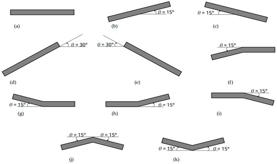
Figure 1.
Geometric configurations for: (a) Case 1; (b) Case 2; (c) Case 3; (d) Case 4; (e) Case 5; (f) Case 6; (g) Case 7; (h) Case 8; (i) Case 9; (j) Case 10; and (k) Case 11.
It is important to note that, since this is a numerical analysis of the operational principle of the SP, the presence of the turbine below the plate, responsible for converting wave energy into electrical energy, will not be considered for this study. Additionally, to standardize the results and maintain the same material costs, the area and thickness of the SP were kept constant across all cases presented in Figure 1.
2.1. Mathematical and Numerical Modeling
This study uses the second-order Stokes wave theory to describe the regular wave behavior, which assumes that the wave height is relatively small compared to its wavelength. This theory accounts for non-linear effects, leading to asymmetries where the wave crest is higher and steeper than the trough. The wave’s velocity components in a 2D approach are defined as [29]:
where u and w are, respectively, the horizontal and vertical components of wave velocity (m/s), g is the gravitational acceleration (m/s2), h is the water depth (m), x is the horizontal position in the domain (m), t is the time (s), z is the depth of a particle in the fluid (m), measured from the surface, H is the wave height (m), and k and ω are the wave number (m−1) and the wave angular frequency (s−1), respectively, given by:
being λ the wavelength (m) and T the wave period (s).
Numerical simulations were conducted using the Fluent CFD software package, version 2024 R2. This software is based on the finite volume method (FVM), which enables numerical simulations of fluid flow and heat transfer in complex geometries [30,31,32].
To handle the water–air flow, the volume of fluid (VOF) multiphase model was adopted to manage the interface between both fluids. In this approach, each phase (water and air) is represented within a computational cell as a volumetric fraction (α), with the sum of the phases in each cell equaling one [14].
Given that, the flow in this numerical study is laminar, incompressible, two-dimensional, and isothermal. Hence, the equations for the conservation of mass, momentum, and volume fraction are, respectively, defined as [33]:
where ρ is the density (kg/m3), is the velocity vector (m/s), p is the pressure (N/m2), μ is the absolute viscosity coefficient (kg/m·s), and is the strain rate tensor (N/m2).
The continuity and momentum equations are solved for the mixture; hence, ρ and μ properties can be represented for the mixture as follows [34]:
To ensure effective control of the numerical simulations, specific numerical parameters were selected based on previous studies. For the momentum equation, the first-order upwind discretization method was applied; the pressure staggering option (PRESTO) scheme was utilized for pressure discretization; the geo-reconstruct scheme was employed to handle the volumetric fraction calculations; and the pressure-implicit splitting of operators (PISO) algorithm managed the pressure–velocity coupling. One can emphasize that this computational model has been successfully used in previous studies, such as Gomes et al. [35], Machado et al. [15], Mocellin et al. [36], Seibt et al. [13], Goulart et al. [37], and Thum et al. [14].
In turn, the computational domain used in this work is based on the SHP by Seibt et al. [13], which defined the optimized geometry (where the ratio between the wave channel length (Lc) and the wavelength (λ) is greater than 1) when considering the device acting as a WEC. Table 1 presents the wave channel dimensions, where Hc is the wave channel height, and hp, ep, Lp, and Ap represent, respectively, the height, thickness, length, and area of the SHP (Case 1, see Figure 1a).

Table 1.
Dimensions of the numerical wave channel and the horizontal SHP [13].
As previously described, the present study evaluates not only the SHP (Case 1) but also ten other cases of the SP with different inclinations (see Figure 1b–k). For all cases, the dimensions of the wave channel and the area and thickness of the SP, as presented in Table 1, were kept constant. The regular waves generated and propagated in the channel have their characteristics presented in Table 2 and are the same as those used in the study by Seibt et al. [13].
Table 2.
Characteristics of the regular waves [13].
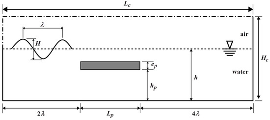
Figure 2.
An illustration of the computational domain.
2.2. Spatial Discretization of the Computational Domain
The computational domain consists of a two-dimensional numerical wave channel with the SP inserted. For spatial discretization, the stretched and bias mesh methodologies were employed. Figure 3 shows a schematic representation of the different regions of the channel, not to scale, along with the mesh methodology used in each of them.
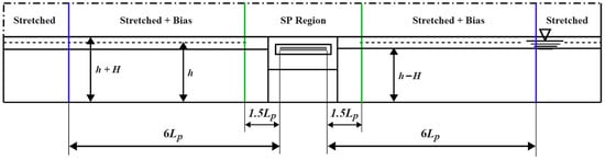
Figure 3.
A schematic of the discretization of the computational domain.
The stretched mesh, as applied in Gomes et al. [35], was used in the upstream and downstream regions (see Figure 3), where a standard number of vertical divisions is applied in the inlet velocity regions. These include the area containing only water (h − H), the region of free surface variation (the interface of water and air phases, from H − h to h + H), and the region above the free surface (containing only air, at h + H). The values for these divisions are 60, 40, and 20, respectively. For horizontal discretization, 50 divisions per wavelength are used. Consequently, quadrilateral computational cells with regular spacing were generated in these regions.
In the SP region (see Figure 3), defined by two vertical green lines located 1.5Lp from the left and right ends of the SP, an irregular mesh with triangular finite volumes was chosen due to the geometric complexity caused by the different inclined geometries for the SP (Cases 2–11, see Figure 1b–k). It is well known that irregular meshes with triangles generally provide less precise results than regular quadrilateral meshes; however, they offer better adaptability to more complex geometric configurations [38], justifying their choice.
The intermediate bias mesh was applied alongside the stretched mesh to smooth the transition to the SP region; this methodology was used between the vertical blue and green lines (stretched + bias in Figure 3). This additional mesh aims to reduce the occurrence of the global Courant error, or floating-point error, often caused by large time steps or abrupt differences in mesh refinement [39,40,41].
Additionally, the region around the SP (see Figure 3) was divided into subareas with the same cell refinement to facilitate discretization and ensure uniformity in the computational cells. This methodology establishes a standard for mesh generation, ensuring that the defined refinement covers the entire extent of the region in which the SP is inserted.
It is worth noting that the stretched mesh for generating regular waves is already a well-established methodology. Thus, the recommendations of Gomes et al. [35] were followed. Since the intermediate bias mesh also follows the vertical divisions of the stretched mesh, it has already been defined as well.
Therefore, the need for mesh convergence studies is evident to determine an irregular triangular mesh suitable for the SP region, bounded by the vertical green lines (see Figure 3), as well as a suitable time step for the global Courant number.
2.3. Boundary Conditions
Figure 4 shows the boundary conditions considered in the numerical wave channel and applied to all the studied cases, where the velocity inlet (red segment) is considered at the left end of the wave channel from the bottom to the free surface, and it represents the second-order Stokes wave generator by means of the imposition of Equations (1) and (2). The wall at the right end of the channel and the surroundings of the SP were defined as rigid walls (black segments). The left superior edge and upper edge of the channel were defined as the pressure outlet (blue segment).
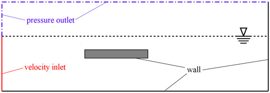
Figure 4.
Schematic illustration of the boundary conditions.
2.4. Mesh and Time Step Convergence Tests
After defining the computational domain geometry, two mesh and two time step convergence studies were conducted to determine the ideal spatial discretization for the SP region (see Figure 3), as well as the ideal time step size for the numerical simulations, aiming to reduce computational costs while maintaining the results accuracy. These studies were based on the computational domain characteristics of Cases 2 and 11 (see Figure 1b–k), which were selected because of their high mesh distortion, ensuring that a sufficiently refined mesh and time step in these cases would provide a reliable standard for the others. Four mesh and five time step configurations were evaluated in these tests, adjusting only the cell size in the SP region, with a time step of 0.01 s for the mesh convergence test, as suggested by Seibt et al. [13]. A quantitative analysis by the relative difference was performed on the maximum absolute axial velocity (umax) below the SP at hp/2 for both tests.
2.5. Verification of the Computational Model
The SHP (Case 1, see Figure 1a) was used for the verification of the computational model. For this purpose, the mesh and time step defined in the previous convergence tests were adopted.
The parameters monitored for the verification of the computational model were the water-free surface elevation (η) upstream of the SHP (at x = 69.792 m, probe 1), the water-free surface elevation downstream of the SP (at x = 248.925 m, probe 2), and the axial velocity (u) under the SHP (at x = 141.9105 m and z = 4.320 m, probe 3). The time step of 0.01 s was used, with a total of 6000 steps, resulting in 60 s of simulation, while the processing time was approximately 4 h.
Further on the comparison will be made qualitatively confronting graphically the results for Case 1 of this article with those from Seibt et al. [13]. Additionally, the quantitative comparison will be carried out, through the statistical indicators mean absolute error (MAE) and root mean square error (RMSE), defined by Botchkarev [42]:
where PS is the value obtained in the present study (here, for Case 1), R is the reference values from Seibt et al. [13], and n is the number of monitored data.
It should be emphasized that the computational model used in Seibt et al. [13] was validated with experimental results by Orer and Ozdamar [23]. Therefore, one can affirm that the verification carried out when comparing the results for the SHP of the present study with those of Seibt et al. [13] indirectly validated the computational model employed in the present study. For this reason and for the sake of brevity, only the verification of the computational model is presented here.
2.6. Analysis of Cases 1–11 Results
As in the numerical model verification (which is Case 1 of Figure 1), the results for the other ten cases were monitored by numerical probes located at the same position early described.
In this way, for the quantitative analysis of the results obtained for the ten cases with inclined geometric configuration of the SP confronting the SHP, the integral of the absolute value (or integral of the magnitude) of the free surface elevation downstream and axial velocity under the device was calculated for each case using the trapezoidal rule [43].
where I is the value of the integral (m or m/s, respectively for η or u), Δt is the time step (s) that is the width of the subintervals, f(φ0) is the function value at the lower limit of the integral (t = 0 s), f(φj) are the function values at intermediate points (0 s < t < 60 s), and f(φn) is the function value at the upper limit of the integral (t = 60 s).
For the comparison of the efficiency as a BW device of the studied cases, the relation Iη1/Iηi, was used, with Iη1 the Case 1 value and Iηi the other case values (for 2 ≤ i ≤ 11). In turn, for the comparison of the efficiency as a WEC device of all cases, the relation Iui/Iu1 was used, in which Iui is the integral value for Cases 2 to 11 (with 2 ≤ i ≤ 1) and Iu1 is the integral value of Case 1. Both as BW and WEC, these dimensionless values directly relate the inclined SP case (Cases 2 to 11) to Case 1 (reference). Therefore, values greater than 1 indicate that the inclined SP is more efficient than the SHP reference case, while values less than 1 indicate less efficiency than the SHP reference case. In addition, it is also possible to compare Cases 2 to 11 among each other, the best and worst being those that present the largest and smallest values, respectively.
3. Results and Discussion
3.1. Mesh Convergence Tests Results
The results for both Cases 2 and 11 (see Figure 1b–k) are presented in Table 3 and Table 4, respectively. Given the relative difference of less than 1% between meshes 2–3 and 3–4 for both Cases 2 and 11, the mesh refinement of the SP region was defined as 0.048 m per computational cell (mesh 3).
Table 3.
Mesh convergence test results for Case 2.
Table 4.
Mesh convergence test results for Case 11.
For improved visualization, Figure 5 plots the results from Table 3 and Table 4, showing the relationship between the total number of volumes used and the maximum axial velocity, as well as the selected spatial discretization (mesh 3, highlighted in red).
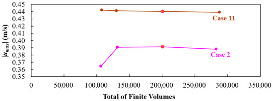
Figure 5.
Mesh convergence tests results.
In order to graphically illustrate the spatial discretization of each numerically simulated computational domain, Figure 6 presents the generated mesh for the eleven cases (see Figure 1). To save space, the upstream and downstream regions of the SP region are included only for Case 1, as these regions are identical for all studied cases.
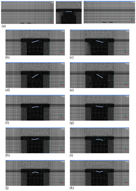
Figure 6.
Mesh discretization results of (a) Case 1; (b) Case 2; (c) Case 3; (d) Case 4; (e) Case 5; (f) Case 6; (g) Case 7; (h) Case 8; (i) Case 9; (j) Case 10; and (k) Case 11.
3.2. Time Step Convergence Tests Results
With the mesh refinement defined, a time-step (Δt) convergence study was conducted to determine a temporal discretization refined enough to accurately simulate the SP fluid dynamic behavior of all studied cases (see Figure 1). Using again Cases 2 and 11 (see Figure 1b–k), four other different time steps were tested, and the obtained results for absolute maximum axial velocity (umax) below the SP, at hp/2, are shown, respectively, in Table 5 and Table 6. In addition, Figure 7 illustrates the results from Table 4 and Table 5.
Table 5.
Time step convergence test results for Case 2.
Table 6.
Time step convergence test results for Case 11.
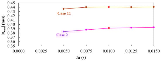
Figure 7.
Time step convergence tests results.
Based on the analysis of Table 5 and Table 6, as well as Figure 7, time step 3, with a value of 0.01 s, was adopted. This time step resulted in the lowest relative percentage error (marked in red in Figure 7), which is the time discretization already used in Seibt et al. [13] and also in the mesh convergence mesh.
3.3. Results of Computational Model’s Verification
Through both qualitative (see Figure 8) and quantitative comparisons (see Table 7) with Seibt et al. [13], it can be considered that the computational model used in this numerical study has been properly verified. This definition is because the generated curves follow the same trend, and the obtained values of RAE and RMSE were low, indicating minimal variation compared to the values from Seibt et al. [13].
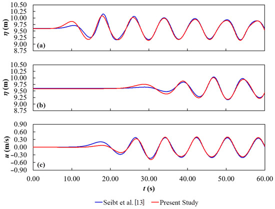
Figure 8.
Results of computational model’s verification: (a) free surface elevation upstream; (b) free surface elevation downstream; and (c) axial velocity below the SP.
Table 7.
RAE and RMSE values for the verification of Seibt et al. [13], during all simulation time.
However, one can observe in Figure 7 that the higher differences occur during the wave stabilization interval. Thereby, Table 8 presents the results comparison after the wave stabilization, achieving still lower values of RAE and RMSE.
Table 8.
RAE and RMSE values for the verification of Seibt et al. [13], after the wave stabilization time.
3.4. Results and Discussion of Cases 1–11
Figure 9, Figure 10 and Figure 11 show the results of Cases 2 to 11, proposed with some inclination for the SP (see Figure 1b–k), plotted together with Case 1 (see Figure 1a), which is the baseline result for comparison in this study. To improve the results visualization, the cases were grouped according to their methodology of variation in the geometric configuration earlier mentioned, always together with the SHP reference case.
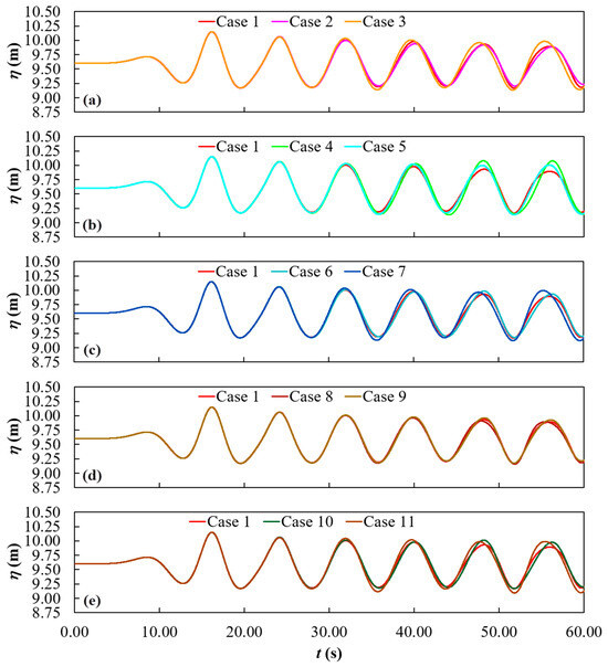
Figure 9.
Results of the free surface elevation upstream of the SP of Cases: (a) 1, 2, 3; (b) 1, 4, 5; (c) 1, 6, 7; (d) 1, 8, 9; and (e) 1, 10, 11.
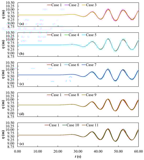
Figure 10.
Results of the free surface elevation downstream of the SP of Cases: (a) 1, 2, 3; (b) 1, 4, 5; (c) 1, 6, 7; (d) 1, 8, 9; and (e) 1, 10, 11.
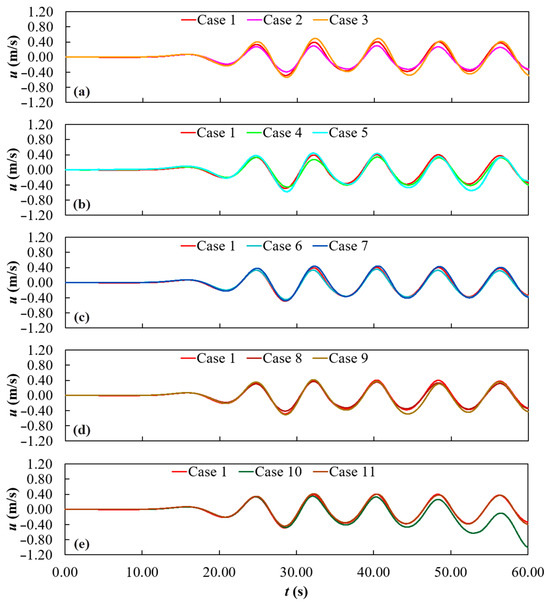
Figure 11.
Results of the axial velocity below the SP of Cases: (a) 1, 2, 3; (b) 1, 4, 5; (c) 1, 6, 7; (d) 1, 8, 9; and (e) 1, 10, 11.
One can observe in Figure 9 that, in general and as expected, there is no significant difference among the water-free surface elevations upstream for the studied SPs. The small variations that occurred are due to the reflection caused by the different geometric configurations of each SP. This aspect indicates that the generation and propagation of the regular waves are being carried out properly.
From Figure 10, it is possible to qualitatively perceive behaviors that are more relevant. For instance, Case 3 (Figure 10a), Case 10 (Figure 10e), and Case 8 (Figure 10d) have a transient variation of the water-free surface elevation, lower, higher, and similar to those in Case 1. Remembering that for its use as BW, a reduction in η is desired.
Figure 11 indicates behaviors even more different among the studied cases, being for SP as WEC necessary an augmentation in axial velocity. Case 11 (Figure 11e) presented a very similar variation than Case 1 for the axial velocity. Case 2 was the one that had the inferior performance, i.e., the highest reduction in magnitude of axial velocity under de SP. Cases 3 (Figure 11a) and 10 (Figure 11e) presented an axial velocity augmentation; however, Case 10 was the only one with a discrepant behavior among all cases. This aspect will be further discussed later.
Despite the important insights from the qualitative evaluation allowed by Figure 9, Figure 10 and Figure 11, a quantitative analysis is essential for a more precise understanding of the influence of SP geometric configurations on its efficiency. Table 9 therefore presents the integral values Iη and Iu for the curves in Figure 10 and Figure 11, respectively, along with the ratios between these integral values for Cases 2 to 11 relative to the corresponding value for Case 1.
Table 9.
Comparison of Iηi and Iui for the 10 inclination cases with the reference case.
Table 9 indicates that the results of the free surface elevation downstream of the SP showed that the inclined SP cases were mostly less efficient than the reference case. However, Cases 2, 3, 7, and 8 are exceptions, achieving values of Iη inferior to Case 1, recommending its use as BW.
Regarding the axial velocity beneath the SP, one can identify in Table 9 that the results of inclined geometries (Cases 2 to 11) were generally superior to Case 1, which is a desired response for its application as WEC. The exceptions are Cases 2, 4, 6, and 8, which had inferior results to Case 1.
Highlights include Cases 3 and 7, which outperformed Case 1 both as a BW and as a WEC, with Case 3 being 11.95% more efficient as a BW and 16.59% more efficient as a WEC, and Case 7 being 8.16% more efficient as a BW and 6.90% more efficient as a WEC.
Based on the results of the integrals, it was possible to define the best and worst cases of geometry variation based on efficiency as a BW and WEC compared to Case 1. As a BW, the best case was Case 3, achieving 11.95% more efficiency than Case 1. As a WEC, the best case was case 10, achieving 19.56% more efficiency than Case 1.
Analyzing the SP based on its multifunctionality as both a BW and WEC, the best case was Case 3. This is the recommended geometric configuration in this study. However, an interesting behavior is observed with Case 10: it achieved superior performance as a WEC while exhibiting the lowest performance as a BW. Thus, Case 10 can be considered for situations where only the WEC functionality is needed.
In order to visualize how the geometric configuration of the SP influences the downstream wave attenuation as a BW and the alternating axial velocity as a WEC, Figure 12 depicts the best, worst, and reference cases for each device function.
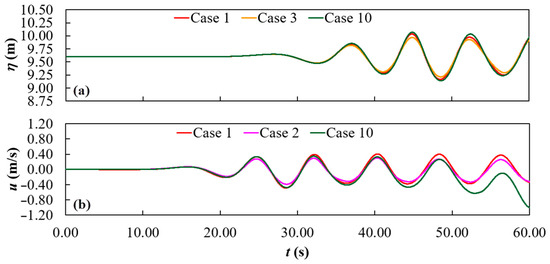
Figure 12.
Comparison among the best, worst, and reference cases for the SP as a: (a) BW and (b) WEC.
The results of Figure 12a evidence the difference among the best (Case 3), worst (Case 4), and reference (Case 1) cases, since Case 3 achieved shorter water-free surface elevations than Case 1 and Case 4. In the same way, it is easy to infer in Figure 12b that Case 10 reached a superior magnitude for the axial velocity under the SP than the reference (Case 1) and the worst (Case 2) geometries.
However, if the BW and WEC functions are taken into account in a concomitant way, the results for the best (Case 3) and worst (Case 4) geometric configurations, together with the reference case (Case 1), are plotted in Figure 13, making it evident that Case 3 conducted to the smaller elevation of the water-free surface after the SP (Figure 13a) and higher axial velocity under the SP, thus reaching superior performance. It is worth highlighting that the worst case was defined among the cases that obtained relative efficiencies lower than 1 for both SP functionalities, being the one that reached the lowest average value between Iη1/Iηi and Iui/Iu1 (see Table 9).
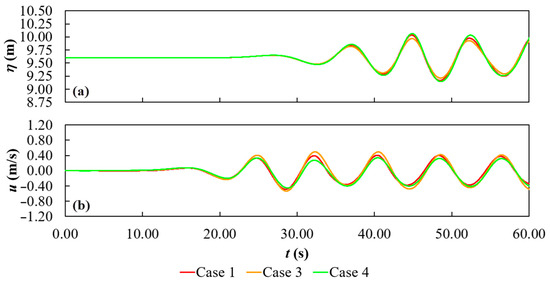
Figure 13.
Comparison among the best, worst, and reference cases for the SP as a BW and WEC simultaneously: (a) downstream water-free surface elevation and (b) water flow axial velocity.
Alongside the integrals Iη and Iu of the probes 1, 2, and 3 results (see Table 9), the ParaView post-processing visualization engine was used to plot the velocity field among the wave channel for 40 s, 50 s, and 60 s (Figure 14, Figure 15, and Figure 16, respectively); with the red color representing water and the blue color representing air. These time values were chosen to have an idea of how the hydrodynamic behavior of the SP varies during the simulation. The cases considered for this additional study were Case 1 (the reference), Case 3 (the case with the best efficiency results), Case 4 (the case with the worst efficiency results), and Case 10 (the case with the unusual yet best axial velocity behavior).
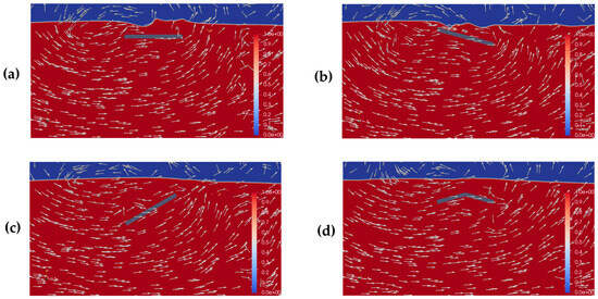
Figure 14.
Velocity field plots at 40 s for: (a) Case 1; (b) Case 3; (c) Case 4; and (d) Case 10.
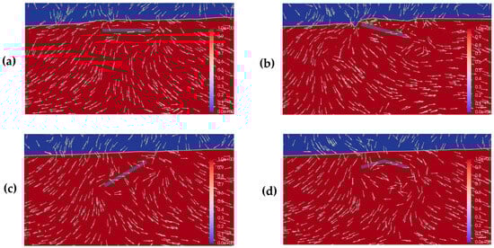
Figure 15.
Velocity field plots at 50 s for: (a) Case 1; (b) Case 3; (c) Case 4; and (d) Case 10.
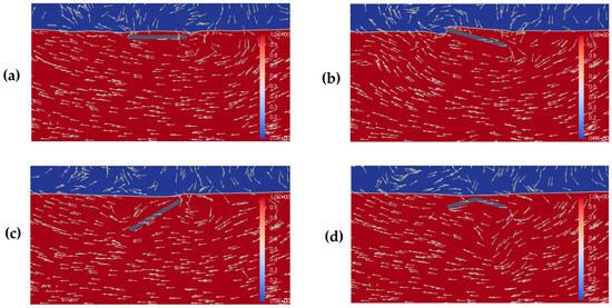
Figure 16.
Velocity field plots at 60 s for: (a) Case 1; (b) Case 3; (c) Case 4; and (d) Case 10.
Cases 1, 3, 4, and 10 (see, respectively, Figure 14a, Figure 14b, Figure 14c, and Figure 14d) showed an expected and approximately similar behavior of axial velocity at 40 s, having a velocity field profile without significant variation below the SP region. However, it is possible to visualize one of the reasons for Case 4’s low BW efficiency: the SP has a limited effect on dissipating the upcoming wave’s energy, as it remains farther from the waves along most of its length, except at its rightmost edge. This increased distance results in less impact of the SP in the incident regular waves.
At 50 s, one of the reasons for the superior performance of Case 3 regarding the WEC becomes evident (see Figure 15b), because the 15° clockwise inclination of the SP causes the incoming waves to deflect downward, resulting in a greater contribution of their velocity components to the axial velocity measured at probe 3. In turn, Cases 1 and 4 (see Figure 15a,c) showed approximately similar velocity fields, and Case 10 (see Figure 15d) started showing a vortex formation below the SP, justifying its higher mean of velocity on the negative axis, especially after 55 s (see Figure 12b).
Additionally, the velocity vectors of Cases 1, 3, and 4 (Figure 16a, Figure 16b, and Figure 16c, respectively) had similar directions for their velocity vectors below the SP at 60 s. Case 10 continued to exhibit vortices in its velocity field beneath the SP, which explains the higher axial velocity reached by this SP geometric configuration (see Figure 12b).
Based on the efficiency results of Cases 3, 5, 7, and 9 (see Table 9), which were more efficient as WECs compared to Case 1, and the discussion of Figure 16b, it can be stated that all the studied clockwise inclination cases demonstrated superior performance as WECs. A possible reason for this superiority is attributed to the downward deflection of the waves, as previously mentioned.
Considering the efficiency results of Cases 2, 3, 7, and 8 (see Table 9), one can infer that all cases with an increased height at one end of the SP demonstrated superior performance as BWs compared to Case 1. This occurs because this geometric alteration reduces the transmission of wave energy, as the raised end of the plate, being closer to the free surface, prevents a part of the wave’s energy from transmitting over the SP, forcing their energy to be dissipated or reflected (see Figure 14c, Figure 15c, and Figure 16c). This effectively reduces the wave amplitude in the region downstream of the structure.
4. Conclusions
Based on the obtained results, it is possible to conclude that SP’s geometric configuration plays a significant role in its hydrodynamic behavior. As observed in the study of the ten cases with some inclination proposed in this work, the variation in the geometric configuration of the SP directly affects its efficiency as both a BW and WEC.
Using Case 1, the SHP, as a reference, it was observed that the geometric configuration can reduce performance by approximately 6.3% (Case 10) as BW and about 18% as WEC (Case 2). However, it was also possible to achieve better performance by approximately 12% as BW and 16.6% as WEC when using Case 3.
These results show that, although some geometric configurations compromise the efficiency of the SP as both a BW and WEC, there are others that result in significant improvements, revealing the potential for optimization through geometric adjustments. Furthermore, if the SP functionalities as a BW and WEC are considered separately, the best performances are obtained by Cases 3 and 10, respectively. However, if both SP functionalities are concomitantly taken into account, the best geometric configuration is Case 3.
Despite the promising results, some limitations should be noted. The use of regular waves and the absence of a numerical beach impose constraints on the study, as does the non-consideration of a turbine beneath the SP and the analysis of only one set of wave characteristics. Moreover, the fixed configuration of the SP did not account for material variations that might influence the results. Future research could address these aspects to provide a more comprehensive evaluation of the device’s efficiency.
Therefore, this numerical study opens the possibility for future investigations on this topic, where more in-depth studies can be conducted regarding the hydrodynamic behavior of the channel, or different scenarios can be considered, such as the incidence of irregular waves, the inclusion of a numerical beach, the use of longer simulation times, or even the analysis of additional cases of geometric variation of the SP, in order to have a more comprehensive analysis of the effect of inclination on the device’s performance.
Author Contributions
Conceptualization, V.E.M. and L.A.I.; methodology, V.E.M., R.A.A.C.G., B.N.M. and L.A.I.; software, V.E.M., G.Ü.T., R.A.A.C.G., B.N.M. and L.A.I.; validation, V.E.M., G.Ü.T. and R.A.A.C.G.; formal analysis, L.A.O.R., E.D.d.S., B.N.M. and L.A.I.; investigation, V.E.M. and L.A.I.; resources, L.A.O.R., E.D.d.S., B.N.M. and L.A.I.; data curation, V.E.M., G.Ü.T., R.A.A.C.G. and L.A.I.; writing—original draft preparation, V.E.M. and L.A.I.; writing—review and editing, V.E.M., L.A.O.R., E.D.d.S., B.N.M. and L.A.I.; visualization, L.A.O.R., E.D.d.S., B.N.M. and L.A.I.; supervision, L.A.I.; project administration, L.A.I.; funding acquisition, L.A.O.R., E.D.d.S., B.N.M. and L.A.I. All authors have read and agreed to the published version of the manuscript.
Funding
This research was funded by the Brazilian Coordination for the Improvement of Higher Education Personnel—CAPES (Finance Code 001), Research Support Foundation of the State of Rio Grande do Sul—FAPERGS (Public Call FAPERGS 07/2021—Programa Pesquisador Gaúcho—PqG—21/2551-0002231-0), Brazilian National Council for Scientific and Technological Development—CNPq (Processes: 125941/2024-2, 309648/2021-1, 307791/2019-0, 308396/2021-9, 440010/2019-5, and 440020/2019-0), and Federal University of Rio Grande do Sul—UFRGS (Edital PROPESQ/UFRGS 2019—Programa Institucional de Auxílio à Pesquisa de Docentes Recém-Contratados pela UFRGS).
Data Availability Statement
Data can be accessed upon request to the authors.
Acknowledgments
The authors thank to CAPES, FAPERGS, CNPq, and UFRGS for financial support.
Conflicts of Interest
The authors declare no conflicts of interest.
Nomenclature
| Ap | area of the SP (m) |
| ep | thickness of SP (m) |
| f(ϕ0) | value of the function at the lower limit of the integral |
| f(ϕj) | function values at intermediate points |
| f(ϕn) | value of the function at the upper limit of the integral |
| g | gravitational acceleration (m/s2) |
| H | wave height (m) |
| h | water depth (m) |
| Hc | wave channel height (m) |
| hp | height of SP (m) |
| I | integral of absolute value (m⋅s or m) |
| Iη | value of the water free surface elevation integral (m) |
| Iu | value of the water flow axial velocity integral (m/s) |
| k | wave number (m−1) |
| Lc | wave channel length (m) |
| Lp | length of SP (m) |
| p | pressure (N/m2) |
| PS | value obtained in the present study (m or m/s) |
| R | reference value (m or m/s) |
| T | wave period (s) |
| t | time (s) |
| u | horizontal component of wave velocity (m/s) |
| umax | maximum axial velocity of the water flow under the SP (m/s) |
| velocity vector (m/s) | |
| x | horizontal position in the domain (m) |
| z | depth of a particle in the fluid (m) |
| w | vertical component of wave velocity (m/s) |
| α | volumetric fraction (-) |
| Δt | time-step (s) |
| η | water free surface elevation (m) |
| λ | wavelength (m) |
| μ | absolute viscosity coefficient (kg/m·s) |
| ρ | fluid density (kg/m3) |
| strain rate tensor (N/m2) | |
| ω | wave angular frequency (s−1) |
References
- IPCC. Sections. In Climate Change 2023: Synthesis Report; Lee, H., Romero, J., Eds.; Contribution of Working Groups I, II and III to the Sixth Assessment Report of the Intergovernmental Panel on Climate Change; IPCC: Geneva, Switzerland, 2023. [Google Scholar] [CrossRef]
- Vallega, G.A. Climate Change and Sea-Level Rise in the Mediterranean: Environmental Impacts and Responses. J. Coast. Res. 2001, 17, 850–857. [Google Scholar]
- May, C.L.; Osler, M.S.; Stockdon, H.F.; Barnard, P.L.; Callahan, J.A.; Collini, R.C.; Ferreira, J.F.H.C.M.; Lentz, E.E.; Mahoney, T.B.; Sweet, W.; et al. Coastal effects. In Fifth National Climate Assessment; Crimmins, A.R., Avery, C.W., Easterling, D.R., Kunkel, K.E., Stewart, B.C., Maycock, T.K., Eds.; U.S. Global Change Research Program: Washington, DC, USA, 2023. [Google Scholar] [CrossRef]
- Shadrick, J.R.; Rood, D.H.; Hurst, M.D.; Piggott, M.D.; Hebditch, B.G.; Seal, A.J.; Wilcken, K.M. Sea-level rise will likely accelerate rock coast cliff retreat rates. Nat. Commun. 2022, 13, 7005. [Google Scholar] [CrossRef] [PubMed]
- International Renewable Energy Agency (IRENA). Renewable Power Generation Costs in 2023; International Renewable Energy Agency: Abu Dhabi, United Arab Emirates, 2024; pp. 49–58. [Google Scholar]
- McKinsey & Company. Global Energy Perspective 2024: Power Outlook. Available online: https://www.mckinsey.com/industries/energy-and-materials/our-insights/global-energy-perspective (accessed on 5 November 2024).
- Thum, G.Ü.; Garozi, V.B.; Maciel, R.P.; dos Santos, E.D.; Seibt, F.M.; Machado, B.N.; Isoldi, L.A. Validation and Verification of Computational Model for the Numerical Simulation of the Operational Principle of a Submerged Horizontal Plate Device. Defect Diffus. Forum 2024, 435, 27–36. [Google Scholar] [CrossRef]
- Dick, T.M.; Brebner, A. Solid and Permeable Submerged Breakwaters. In 11th Coastal Engineering Conference (ASCE 2); ASCE: Reston, VA, USA, 1968; pp. 1141–1158. [Google Scholar] [CrossRef]
- Graw, K.U. The Submerged Plate Wave Energy Converter: A New Type of Wave Energy Device. In Proceedings of the International Symposium on Ocean Energy Development (ODEC), Muroran, Japan, 26–27 August 1993. [Google Scholar]
- Yang, Y.; Zhang, K.; Li, C.; Hao, X.; Xiao, J.; Liu, W. An experimental investigation of wave forces on a submerged horizontal plate over a simple slope. J. Mar. Sci. Eng. 2020, 8, 507. [Google Scholar] [CrossRef]
- Cummins, C.P.; Scarlett, G.T.; Windt, C. Numerical analysis of wave-structure interaction of regular waves with surface-piercing inclined plates. J. Ocean. Eng. Mar. Energy 2022, 8, 99–115. [Google Scholar] [CrossRef]
- Zheng, Y.; Zhou, Y.; Jin, R.; Mu, Y.; He, M.; Zhao, L. Experimental Study on Submerged Horizontal Perforated Plates under Irregular Wave Conditions. Water 2023, 15, 3015. [Google Scholar] [CrossRef]
- Seibt, F.M.; Dos Santos, E.D.; Isoldi, L.A.; Rocha, L.A.O. Constructal Design on Full-Scale Numerical Model of a Submerged Horizontal Plate-Type Wave Energy Converter. Mar. Syst. Ocean Technol. 2023, 18, 1–13. [Google Scholar] [CrossRef]
- Thum, G.Ü.; Maciel, R.P.; Oleinik, P.H.; Rocha, L.A.O.; Santos, E.D.; Seibt, F.M.; Machado, B.N.; Isoldi, L.A. Numerical Analysis of the Submerged Horizontal Plate Device Subjected to Representative Regular and Realistic Irregular Waves of a Sea State. Fluids 2024, 9, 188. [Google Scholar] [CrossRef]
- Machado, B.N.; Oleinik, P.H.; Kirinus, E.P.; Rocha, L.A.O.; Gomes, M.N.; Conde, J.M.P.; Isoldi, L.A. WaveMIMO Methodology: Numerical Wave Generation of a Realistic Sea State. J. Appl. Comput. Mech. 2021, 7, 2129–2148. [Google Scholar] [CrossRef]
- Siew, P.F.; Hurley, D.G. Long Surface Waves Incident on a Submerged Horizontal Plate. J. Fluid Mech. 1977, 83, 141–151. [Google Scholar] [CrossRef]
- Wang, K.H.; Shen, Q. Wave Motion over a Group of Submerged Horizontal Plates. Int. J. Eng. Sci. 1999, 37, 703–715. [Google Scholar] [CrossRef]
- Yu, X. Functional Performance of a Submerged and Essentially Horizontal Plate for Offshore Wave Control: A Review. Coast. Eng. J. 2002, 44, 127–147. [Google Scholar] [CrossRef]
- Aghili, M.; Ghadimi, P.; Maghrebi, Y.F.; Nowruzi, H. Simulating the Interaction of Solitary Wave and Submerged Horizontal Plate Using SPH Method. Int. J. Phys. Res. 2014, 2, 16–26. [Google Scholar] [CrossRef][Green Version]
- Karmakar, D.; Soares, C.G. Wave Motion Control Over Submerged Horizontal Plates. In Proceedings of the ASME 2015 34th ed.; International Conference on Ocean, Offshore and Arctic Engineering, St. John’s, NL, Canada, 31 May–5 June 2015. [Google Scholar] [CrossRef]
- Cheng, Y.; Ji, C.; Ma, Z.; Zhai, G.; Oleg, G. Numerical and Experimental Investigation of Nonlinear Focused Waves-Current Interaction with a Submerged Plate. Ocean Eng. 2017, 135, 11–27. [Google Scholar] [CrossRef]
- Fang, Q.; Yang, C.; Guo, A. Hydrodynamic Performance of Submerged Plates During Focused Waves. J. Mar. Sci. Eng. 2019, 7, 389. [Google Scholar] [CrossRef]
- Carter, W.R. Wave Energy Converters and a Submerged Horizontal Plate. Master’s Thesis, Ocean and Resources Engineering, University of Hawaii, Honolulu, HI, USA, 2005. [Google Scholar]
- Orer, G.; Ozdamar, A. An Experimental Study on the Efficiency of the Submerged Plate Wave Energy Converter. Renew Energy 2007, 32, 1317–1327. [Google Scholar] [CrossRef]
- Wagner, J.J.; Wagner, J.R.; Hayatdavoodi, M. Hydrodynamic analysis of a submerged wave energy converter. In Proceedings of the 4th Marine Energy Technology Symposium METS2016, Washington, DC, USA, 25–27 April 2016. [Google Scholar] [CrossRef]
- Xu, Y.; Zhang, G.; Wan, D.; Chen, G. MPS Method for Study of Interactions between Solitary Wave and Submerged Horizontal Plate. In Proceedings of the 29th International Ocean and Polar Engineering Conference, Honolulu, HI, USA, 16–21 June 2019. [Google Scholar] [CrossRef]
- Hayatdavoodi, M.; Ertekin, R.C.; Valentine, B.D. Solitary and Cnoidal Wave Scattering by a Submerged Horizontal Plate in Shallow Water. AIP Adv. 2017, 7, 065212. [Google Scholar] [CrossRef]
- He, M.; Gao, X.; Xu, W.; Ren, B.; Wang, H. Potential Application of Submerged Horizontal Plate as a Wave Energy Breakwater: A 2D Study Using the WCSPH Method. Ocean Eng. 2019, 185, 27–46. [Google Scholar] [CrossRef]
- Dean, R.G.; Dalrymple, R.A. Water Wave Mechanics for Engineers and Scientists. Adv. Ser. Ocean Eng. 1991, 2, 305. [Google Scholar] [CrossRef]
- ANSYS, Inc. Ansys Fluent Theory Guide; ANSYS, Inc.: Canonsburg, PA, USA, 2013. [Google Scholar]
- Patankar, S.V. Numerical Heat Transfer and Fluid Flow; McGraw-Hill: New York, NY, USA, 1980. [Google Scholar]
- Versteeg, H.K.; Malalasekera, W. An Introduction to Computational Fluid Dynamics—The Finite Volume Method; Pearson Education Limited: London, UK, 2007. [Google Scholar]
- Rafiee, A.; Dutykh, D.; Dias, F. Numerical Simulation of Wave Impact on a Rigid Wall Using a Two-phase Compressible SPH Method. Procedia IUTAM 2015, 18, 123–137. [Google Scholar] [CrossRef]
- Srinivasan, V.; Salazar, A.J.; Saito, K. Modeling the Disintegration of Modulated Liquid Jets Using Volume-of-Fluid (VOF) Methodology. Appl. Math. Model. 2011, 35, 3710–3730. [Google Scholar] [CrossRef]
- Gomes, M.N.; Lorenzini, G.; Rocha, L.A.; dos Santos, E.D.; Isoldi, L.A. Constructal Design Applied to the Geometric Evaluation of an Oscillating Water Column Wave Energy Converter Considering Different Real Scale Wave Periods. J. Eng. Thermophys. 2018, 27, 173–190. [Google Scholar] [CrossRef]
- Mocellin, A.P.G.; Maciel, R.P.; Oleinik, P.H.; dos Santos, E.D.; Rocha, L.A.O.; Ziebell, J.S.; Isoldi, L.A.; Machado, B.N. Geometrical Analysis of an Oscillating Water Column Converter Device Considering Realistic Irregular Wave Generation with Bathymetry. J. Exp. Theor. Anal. 2023, 1, 24–43. [Google Scholar] [CrossRef]
- Goulart, M.M.; Martins, J.C.; Gomes, A.P.; Puhl, E.; Rocha, L.A.O.; Isoldi, L.A.; das Gomes, M.N.; dos Santos, E.D. Experimental and numerical analysis of the geometry of a laboratory-scale overtopping wave energy converter using constructal design. Renew. Energy 2024, 236, 121497. [Google Scholar] [CrossRef]
- ANSYS, Inc. Meshing User’s Guide; ANSYS Help: Canonsburg, PA, USA, 2024. [Google Scholar]
- Mann, D. Multiphase Flow, CFD, and Courant Number. Siemens Digital Industries Software, Simcenter Blog, 2024. Available online: https://blogs.sw.siemens.com/simcenter/multiphase-flow-cfd-and-courant-number/ (accessed on 2 November 2024).
- SimFlow. Courant Number in CFD. SimFlow. Available online: https://sim-flow.com/courant-number-in-cfd/ (accessed on 15 November 2024).
- Ideal Simulations. Courant Number in CFD. Ideal Simulations. Available online: https://www.idealsimulations.com/resources/courant-number-cfd/ (accessed on 15 November 2024).
- Botchkarev, A. Performance Metrics (Error Measures) in Machine Learning Regression, Forecasting and Prognostics: Properties and Typology. Interdiscip. J. Inf. Knowl. Manag. 2019, 14, 45–79. [Google Scholar] [CrossRef]
- Chapra, S.C.; Canale, R.P. Numerical Methods for Engineers, 7th ed.; McGraw-Hill Education: New York, NY, USA, 2015. [Google Scholar]


Disclaimer/Publisher’s Note: The statements, opinions and data contained in all publications are solely those of the individual author(s) and contributor(s) and not of MDPI and/or the editor(s). MDPI and/or the editor(s) disclaim responsibility for any injury to people or property resulting from any ideas, methods, instructions or products referred to in the content. |
© 2025 by the authors. Licensee MDPI, Basel, Switzerland. This article is an open access article distributed under the terms and conditions of the Creative Commons Attribution (CC BY) license (https://creativecommons.org/licenses/by/4.0/).