Waveguide Quantum Electrodynamics: Tryptophans Entangled with Water as Data Qubits in a Microtubule

Abstract

In this paper, we introduce waveguide Quantum Electrodynamics (wQED) for the description of tryptophans in microtubules representing data qubits for information storage and, possibly, information processing. We propose a Hamiltonian in wQED and derive Heisenberg equations for qubits and photons. Using the Heisenberg equations, we derive time-evolution equations for the probability of qubits and the distribution of photons both at zero and finite temperature. We then demonstrate the resultant sub-radiance with small decay rates, which is required to achieve robust data qubits for information storage by coupling tryptophan residues containing data qubits with water molecules as Josephson quantum filters (JQFs). We also describe an oscillation processes of qubits in a tubulin dimer through the propagation of excitations with changing decay rates of JQFs. Data qubits are found to retain initial values by adopting sub-radiant states involving entanglement with water degrees of freedom.

1. Introduction

What is the physical mechanism of memory, and where does the brain store our memories? These are still open questions. In conventional neuroscience, the synaptic plasticity among neurons corresponds to memories stored in a brain by strengthening the connections involved in more frequent signal transmission resulting from specific activities. External stimulations change synaptic signaling and enhance signal transfer among neurons, which is called long-term potentiation. However, if synaptic plasticity is required for storage of memory, how do we explain memory in single-cell organisms [1]? To explain memory storage, even for single-cell organisms, we need to include molecular mechanisms involving the cytoskeleton structures inside cells whose organization of internal degrees of freedom could serve as memory storage mechanisms, as previously proposed by others [2]. Furthermore, it is important to briefly discuss the issue of energy efficiency characterizing the human brain. We require, on average, $20 \mathrm{W}$ of power for the brain to function under normal circumstances, which is extremely small compared with man-made computational technology, with a power demand as high as $250 \mathrm{kW}$ (we refer to [3]) for AlphaGo in DeepMind, where a human won one of five games, in spite of the orders-of-magnitude difference in the respective power needs. How do we realize this extremely high energy efficiency for information processing taking place in the brain within the framework of classical information processing? This is a major challenge. We propose a different approach to resolve this issue. Our strategy is to adopt quantum information processing and quantum information storage in the cytoskeleton.

Cellular cytoskeletons construct a network of proteins that are indispensable for the performance of key cellular processes involving growth, molecular transport, internal structural reorganization, cell division and motility, as shown by Lee et al. [4]. We find microfilaments (also referred to as actin filaments), intermediate filaments and microtubules as the main components of cytoskeletons. Tryptophans in microtubules can play the role of information processors. Craddock et al. suggested that high-capacity memory storage can be achieved in microtubules by CaMKII phosphorylation of specific residues in its building blocks, namely tubular dimers [2]. Additionally, biophoton mechanisms may play a role in fast intra- and inter-cellular communication, since both super-radiant (fast decay) and sub-radiant (slow decay) states have been experimentally determined to emerge for tryptophan excitations, as shown in [5,6,7]. Moreover, Babcock et al. investigated tryptophan mega-networks in microtubules, where super-radiant processes can emerge, even under thermal equilibrium conditions [8]. Super-radiant photon emission can lead to quantum information transfer, as two separate quantum dots conduct photonic information processing, as shown in an experimental study [9]. Super-radiance realizes long-range atom–atom interactions under conditions where atoms are confined to one spatial dimension [10]. Furthermore, since microtubules are surrounded by mitochondria, the production of reactive oxygen species (ROS) by mitochondria (as a byproduct of ATP-based energy production) can generate ultra-weak photon emission within cells [11]. Since microtubules have been shown to absorb these photons, store them for a period of time and release them into the environment by de-excitation, microtubule networks may act to transfer and, perhaps, process ROS-generated photons that may contain quantum information (qubits). Zapata et al. suggested ultra-weak photon emission due to oxidative stress [12]. Shirmovsky studied quantum entanglement in microtubule tryptophan systems [13,14]. Moreover, circadian clock activity might be explained by photo-reduction mediated by tryptophan [15].

Additionally, water degrees of freedom might play a role, due to their dipole moments, by extending local events occurring in microtubules to diffused, non-local events in distal regions of the brain. In fact, quantum brain dynamics, which is a Quantum Field Theory (QFT) of water electric dipoles and photon degrees of freedom, represents a mathematically developed hypothesis of memory formation in such a system. It originated with the work reported in [16,17,18]. The QFT approach to biological systems was also further elaborated on in the 1980s in a series of seminal papers [19,20,21,22,23]. Water and photon degrees of freedom were explicitly introduced in QBD by Jibu and Yasue [24]. These degrees of freedom might amplify the effects of polarization of dipoles in biological systems, namely tryptophan residues abundantly present in microtubules, and may extend local events taking place in tubulin’s tryptophans to non-local information diffused in the whole brain. Then, information contained in the local events might be converted to non-local holographic information. The holographic approach was first proposed by Pribram [25,26], who was a collaborator of Jibu and Yasue. We described holography within the framework in QBD in our earlier work [27,28,29], where rotational degrees of freedom of water molecules were adopted. 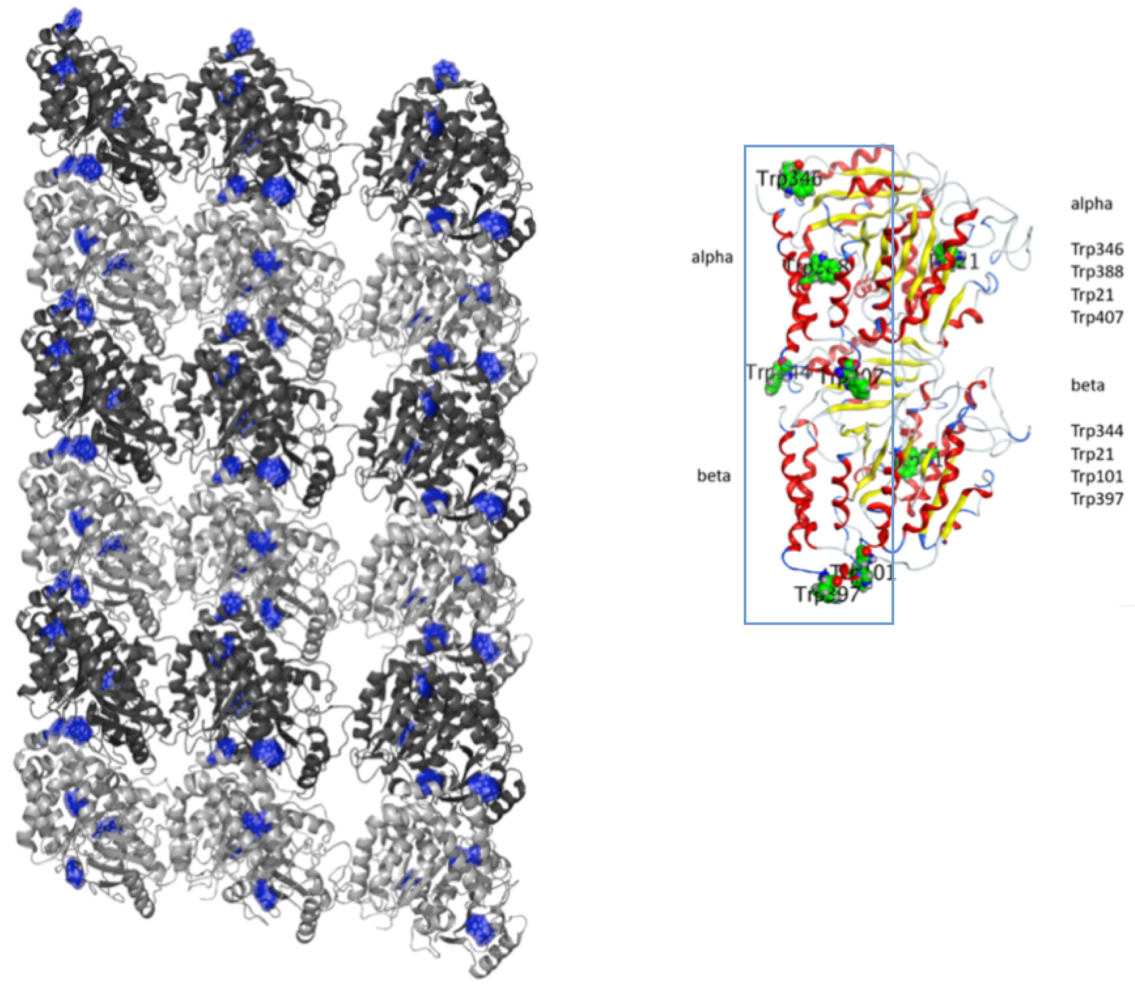Super-radiant photon emission might be viewed as coherent light for interference patterns (for holography) of reference waves and object waves irradiated on microtubules [30,31,32]. We consider tryptophans in microtubules as candidates for local memory in the brain. As shown in Figure 1, we find that six (of eight) tryptophans in a tubulin dimer form a one-dimensional waveguide; then, we can adopt waveguide quantum electrodynamics, where qubits with two energy levels are coupled with photon modes in one spatial dimension. Tryptophans might also be entangled with surrounding water molecules. Here, we can adopt properties of water molecules for absorption and emission in a large variety of wavelengths, especially with the same frequency of absorption for water molecules (electronically resonant mode) as that of tryptophans. Finally, a recent paper indicated an important role of membrane dipoles in neutrons as participants in holographic image formation in the brain [33].

In this paper, we consider tryptophan residues in a microtubule lattice as data qubits entangled with surrounding water molecules that can be utilized for memory storage in a brain. Typically, a microtubule consists of 13 protofilaments involving tubulin dimers as their building blocks. We consider a protofilament as a potential waveguide for propagating photons among qubits aligned in one dimension. We aim to investigate the robustness of tryptophan data qubits entangled with water molecules as Josephson quantum filters adopting sub-radiance. We first introduce a Hamiltonian within the framework of waveguide quantum electrodynamics involving qubits coupled with several photon modes. Next, we adopt Heisenberg equations for operators and derive time-evolution equations for probability coefficients in both zero- and finite-temperature cases. Using the time-evolution equations, we show the robustness of data qubits coupled with Josephson quantum filters that correspond to water molecules in our numerical simulations. Sub-radiance is found to be a key concept for the resultant robustness.

This paper is organized as follows. In Section 2, we show time-evolution equations using Heisenberg equations derived using the Hamiltonian of waveguide QED. In Section 3, we show numerical results illustrating the robustness of data qubits. In Section 4, we discuss our results. In Section 5, we provide concluding remarks and future perspectives. In this paper, we use the natural units where the speed of light, the Planck constant (ℏ) and the Boltzmann constant are all set to unity.

2. Time-Evolution Equations at Zero and Finite Temperature

In this section, we provide time-evolution equations in waveguide QED [34] at zero and finite temperature. The degrees of freedom are qubits involving the ground state ($|0\rangle$) and an excited state ($|1\rangle$), as well as photons coupled with qubits arranged in $1+1$ dimensions.

We begin with the Hamiltonian,

$$\begin{array}{c}\hfill H=\sum _j{\omega }_j{\sigma }_j^{†}{\sigma }_j+{\int }_0^{\infty }dkk{c}_k^{†}{c}_k+\sum _j{\int }_0^{\infty }dk\left[{\xi }_{jk}{\sigma }_j^{†}{c}_k+{\xi }_{jk}^{*}{c}_k^{†}{\sigma }_j\right],\end{array}$$

(1)

where we introduce

$$\begin{array}{c}\hfill {\sigma }_j^{†}=\left(\begin{array}{cc}0& 1\\ 0& 0\end{array}\right),{\sigma }_j=\left(\begin{array}{cc}0& 0\\ 1& 0\end{array}\right)\mathrm{for}j\mathrm{th}\mathrm{qubit},\end{array}$$

(2)

as well as creation and annihilation operators for photons with momentum (k) by $c_k^{†}$ and $c_k$. The integration in $\int dk$ is set from $-\infty$ to ∞ or from 0 to ∞. We introduce coupling (${\xi }_j$) between qubits and photons as follows:

$$\begin{array}{c}\hfill {\xi }_{jk}=\sqrt{{\displaystyle \frac{{\gamma }_j}{\pi }}}cos(k{r}_j+\theta ),\end{array}$$

(3)

where ${\gamma }_j$ represents the decay rate of the jth qubit in position $r_j$ in one spatial dimension and $\theta$ represents the boundary condition for the coupling. We find the commutation relations for these operators as follows:

$$\begin{array}{c}\hfill [{\sigma }_j,{\sigma }_l^{†}]={\delta }_{jl}(1-2{\sigma }_j^{†}{\sigma }_j),\end{array}$$

(4)

$$\begin{array}{c}\hfill [c_p,c_q^{†}]=\delta (p-q).\end{array}$$

(5)

The commutations between two creation operators and between two annihilation operators are zero.

In the Heisenberg representation, we find Heisenberg equations and the corresponding Hermitian conjugates as follows:

$$\begin{array}{ccc}i{\displaystyle \frac{d{\sigma }_j\left(t\right)}{dt}}\hfill & =& [{\sigma }_j\left(t\right),H\left(t\right)]\hfill \\ & =& {\omega }_j\left(1-2{\sigma }_j^{†}\left(t\right){\sigma }_j\left(t\right)\right){\sigma }_j\left(t\right)+{\int }_0^{\infty }dk{\xi }_{jk}{c}_k\left(t\right)\left(1-2{\sigma }_j^{†}\left(t\right){\sigma }_j\left(t\right)\right),\hfill \end{array}$$

(6)

$$\begin{array}{ccc}i{\displaystyle \frac{d{c}_k\left(t\right)}{dt}}\hfill & =& [c_k\left(t\right),H\left(t\right)]\hfill \\ & =& k{c}_k\left(t\right)+\sum _j{\xi }_{jk}^{*}{\sigma }_j\left(t\right).\hfill \end{array}$$

(7)

We then investigate relaxation processes at zero temperature. The initial state involving excitation present only in the first qubit including ${|1\rangle }_1$ is given by

$$\begin{array}{c}\hfill |\psi \left(0\right)\rangle ={\sigma }_1^{†}\left(0\right)|v\rangle ,\end{array}$$

(8)

with the ground state being $|v\rangle ={\prod }_j{|0\rangle }_j\otimes {|\mathrm{vac}\rangle }_{\mathrm{photons}}$ with ${\sigma }_j\left(0\right)|v\rangle =0$, $c_p\left(0\right)|v\rangle =0$. Due to the Schrödinger equation, we can write

$$\begin{array}{ccc}\hfill |\psi (t)\rangle & =& e^{-iHt}|\psi \left(0\right)\rangle \hfill \\ & =& \sum _j{\alpha }_j\left(t\right){\sigma }_j^{†}\left(0\right)|v\rangle +\int dkF(k,t)c_k^{†}\left(0\right)|v\rangle .\hfill \end{array}$$

(9)

We then find

$$\begin{array}{ccc}\hfill {\alpha }_j\left(t\right)& =& \langle v|{\sigma }_j\left(0\right)|\psi \left(t\right)\rangle \hfill \\ & =& \langle v|{\sigma }_j\left(0\right)e^{-iHt}{\sigma }_1^{†}\left(0\right)|v\rangle \hfill \\ & =& \langle v|e^{-iHt}{e}^{iHt}{\sigma }_j\left(0\right)e^{-iHt}{\sigma }_1^{†}\left(0\right)|v\rangle \hfill \\ & =& \langle v|{\sigma }_j\left(t\right){\sigma }_1^{†}\left(0\right)|v\rangle ,\hfill \end{array}$$

(10)

with $\langle v|H=0$. Similarly, we find

$$\begin{array}{ccc}\hfill F(k,t)& =& \langle v|c_k\left(0\right)|\psi \left(t\right)\rangle \hfill \\ & =& \langle v|c_k\left(t\right){\sigma }_1^{†}\left(0\right)|v\rangle .\hfill \end{array}$$

(11)

Using Heisenberg Equations (6) and (7), we then derive the following relationship:

$$\begin{array}{ccc}\hfill i{\displaystyle \frac{d{\alpha }_j\left(t\right)}{dt}}& =& \langle v|i{\displaystyle \frac{d{\sigma }_j\left(t\right)}{dt}}{\sigma }_1^{†}\left(0\right)|v\rangle \hfill \\ & =& \langle v|\left({\omega }_j{\sigma }_j\left(t\right){\sigma }_1^{†}\left(0\right)+\int dk{\xi }_{jk}{c}_k\left(t\right)\left(1-2{\sigma }_j^{†}\left(t\right){\sigma }_j\left(t\right)\right){\sigma }_1^{†}\left(0\right)\right)|v\rangle \hfill \\ & =& {\omega }_j{\alpha }_j\left(t\right)+\int dk{\xi }_{jk}F(k,t),\hfill \end{array}$$

(12)

$$\begin{array}{ccc}\hfill i{\displaystyle \frac{dF(k,t)}{dt}}& =& \langle v|i{\displaystyle \frac{d{c}_k\left(t\right)}{dt}}{\sigma }_1^{†}\left(0\right)|v\rangle \hfill \\ & =& \langle v|\left(k{c}_k\left(t\right)+\sum _j{\xi }_{jk}^{*}{\sigma }_j\left(t\right)\right){\sigma }_1^{†}\left(0\right)|v\rangle \hfill \\ & =& kF(k,t)+\sum _j{\xi }_{jk}^{*}{\alpha }_j\left(t\right).\hfill \end{array}$$

(13)

In the above equations, we obtain the conservation law for excitation numbers as follows:

$$\begin{array}{c}\hfill {\displaystyle \frac{d}{dt}}\left[\sum _j\left({\alpha }_j^{*}\left(t\right){\alpha }_j\left(t\right)\right)+\int dk{F}^{*}(k,t)F^{*}(k,t)\right]=0,\end{array}$$

(14)

where ${\alpha }_j^{*}\left(t\right){\alpha }_j\left(t\right)$ represents the occupation probability of state ${|1\rangle }_j$ and $F^{*}(k,t)F(k,t)$ is related to the distribution of photons with momentum (k) at time t.

The solution of $F(k,t)$ in Equation (13) is

$$\begin{array}{c}\hfill F(k,t)=-i\sum _j\sqrt{{\displaystyle \frac{{\gamma }_j}{\pi }}}cos(k{r}_j+\theta ){\int }_0^{t}d{t}^{\prime }{\alpha }_j\left(t^{\prime }\right)e^{-ik(t-t^{\prime })}.\end{array}$$

(15)

Setting the lower bound of k from zero to $-\infty$ and using the solution of $F(k,t)$, we then expand Equation (12) as

$$\begin{array}{ccc}\hfill i{\displaystyle \frac{d{\alpha }_j\left(t\right)}{dt}}& =& {\omega }_j{\alpha }_j\left(t\right)-i{\int }_{-\infty }^{\infty }dk\sqrt{{\displaystyle \frac{{\gamma }_j}{\pi }}}cos(k{r}_j+\theta )\sum _l\sqrt{{\displaystyle \frac{{\gamma }_l}{\pi }}}cos(k{r}_l+\theta ){\int }_0^{t}d{t}^{\prime }{\alpha }_l\left(t^{\prime }\right)e^{-ik(t-t^{\prime })}\hfill \\ & =& {\omega }_j{\alpha }_j\left(t\right)-i\sum _l{\displaystyle \frac{\sqrt{{\gamma }_j{\gamma }_l}}{2}}{\int }_0^{t}d{t}^{\prime }{\alpha }_l\left(t^{\prime }\right)\hfill \\ & & \times [\delta (r_j+r_l-(t-t^{\prime }))e^{2i\theta }+\delta (r_j-r_l-(t-t^{\prime }))\hfill \\ & & +\delta (-r_j+r_l-(t-t^{\prime }))+\delta (-r_j-r_l-(t-t^{\prime }))e^{-2i\theta }]\hfill \\ & =& {\omega }_j{\alpha }_j\left(t\right)-i\sum _l{\displaystyle \frac{\sqrt{{\gamma }_j{\gamma }_l}}{2}}[{\Theta }_{r_j+r_l\in (0,t)}{\alpha }_l(t-(r_j+r_l))e^{2i\theta }\hfill \\ & & +{\Theta }_{r_l-r_j\in (0,t)}{\alpha }_l(t-(r_l-r_j))+{\Theta }_{r_j-r_l\in (0,t)}{\alpha }_l(t-(r_j-r_l))\hfill \\ & & +{\Theta }_{-r_j-r_l\in (0,t)}{\alpha }_l(t+(r_j+r_l))e^{-2i\theta }],\hfill \end{array}$$

(16)

If the limits of integration over k are from 0 to ∞, we require the ${\displaystyle \frac{1}{2}}$ factor to be multiplied by the second term on the right-hand side of the above equation. The first term on the right-hand side represents the frequency term, while the second term involves the decay factors ($\sqrt{{\gamma }_j{\gamma }_l}$). The damping oscillation for the excitation of a qubit is found to emerge in time evolution.

We now extend our approach to quantum dynamics at finite temperature. The initial density matrix ($\rho \left(0\right)$) is represented by

$$\begin{array}{c}\hfill \rho \left(0\right)={\sigma }_1^{†}\left(0\right){\rho }_{\mathrm{eq}}{\sigma }_1\left(0\right),{\rho }_{\mathrm{eq}}={\displaystyle \frac{e^{-\beta H_{\mathrm{ph}}}\otimes |v_a\rangle \langle v_a|}{\mathrm{tr}\left(e^{-\beta H_{\mathrm{ph}}}\otimes |v_a\rangle \langle v_a|\right)}},\end{array}$$

(17)

with $H_{\mathrm{ph}}=\int dkk{c}_k^{†}{c}_k$ and the ground state of qubits ($|v_a\rangle$). We consider a heat bath of photons with a temperature of $T={\beta }^{-1}$. Since unitary evolution emerges for the density matrix, we write

$$\begin{array}{ccc}\hfill \rho \left(t\right)& =& e^{-iHt}{\sigma }_1^{†}\left(0\right){\rho }_{\mathrm{eq}}{\sigma }_1\left(0\right)e^{iHt}\hfill \\ & =& \left(\sum _j{\alpha }_j\left(t\right){\sigma }_j^{†}\left(0\right)+{\int }_0^{\infty }dkF(k,t)c_k^{†}\left(0\right)\right){\rho }_{\mathrm{eq}}\left(\sum _m{\alpha }_m^{*}\left(t\right){\sigma }_m\left(0\right)+{\int }_0^{\infty }d{k}^{\prime }{F}^{*}(k^{\prime },t)c_{k^{\prime }}\left(0\right)\right).\hfill \end{array}$$

(18)

Here, $\left({\sum }_j{\alpha }_j\left(t\right){\sigma }_j^{†}\left(0\right)+{\int }_0^{\infty }dkF(k,t)c_k^{†}\left(0\right)\right)$ represents the projection onto the state involving one excitation, which is the approximation adopted in our approach. The excitation numbers for the density matrix are written as

$$\begin{array}{ccc}\hfill \mathrm{tr}\rho \left(t\right)& =& \sum _j{|{\alpha }_j\left(t\right)|}^2+\int dkd{k}^{\prime }F(k,t)F^{*}(k^{\prime },t)\left(\delta (k-k^{\prime })+\mathrm{tr}\left(c_k^{†}\left(0\right)c_{k^{\prime }}\left(0\right){\rho }_{\mathrm{eq}}\right)\right)\hfill \\ & =& \sum _j|{\alpha }_j{\left(t\right)|}^2+\int dk{|F(k,t)|}^2(1+n_k),\hfill \end{array}$$

(19)

with the Bose–Einstein distribution ($n_k={\displaystyle \frac{1}{e^{\beta k}-1}}$) for temperature ($T={\beta }^{-1}$).

We can also introduce the other elements of the density matrix as

$$\begin{array}{ccc}\hfill \mathrm{tr}\left({\sigma }_j\left(0\right)\rho \left(t\right){\sigma }_m^{†}\left(0\right)\right)& =& \mathrm{tr}\left(\left(e^{-iHt}{e}^{iHt}\right){\sigma }_j\left(0\right)\left(e^{-iHt}{\sigma }_1^{†}\left(0\right){\rho }_{\mathrm{eq}}{\sigma }_1\left(0\right)e^{iHt}\right){\sigma }_m^{†}\left(0\right)\left(e^{-iHt}{e}^{iHt}\right)\right)\hfill \\ & =& \mathrm{tr}\left({\sigma }_j\left(t\right){\sigma }_1^{†}\left(0\right){\rho }_{\mathrm{eq}}{\sigma }_1\left(0\right){\sigma }_m^{†}\left(t\right)\right)\hfill \\ & =& {\alpha }_j\left(t\right){\alpha }_m^{*}\left(t\right),\hfill \end{array}$$

(20)

$$\begin{array}{ccc}\hfill \mathrm{tr}\left(c_p\left(0\right)\rho \left(t\right){\sigma }_m^{†}\left(0\right)\right)& =& \mathrm{tr}\left(c_p\left(t\right){\sigma }_1^{†}\left(0\right){\rho }_{\mathrm{eq}}{\sigma }_1\left(0\right){\sigma }_m^{†}\left(t\right)\right)\hfill \\ & =& F(p,t)(1+n_p){\alpha }_m^{*}\left(t\right),\hfill \end{array}$$

(21)

$$\begin{array}{ccc}\hfill \mathrm{tr}\left({\sigma }_j\left(0\right)\rho \left(t\right)c_q^{†}\left(0\right)\right)& =& \mathrm{tr}\left({\sigma }_j\left(t\right){\sigma }_1^{†}\left(0\right){\rho }_{\mathrm{eq}}{\sigma }_1\left(0\right)c_q^{†}\left(t\right)\right)\hfill \\ & =& {\alpha }_j\left(t\right)F^{*}(q,t)(1+n_q),\hfill \end{array}$$

(22)

$$\begin{array}{ccc}\hfill \mathrm{tr}\left(c_p\left(0\right)\rho \left(t\right)c_q^{†}\left(0\right)\right)& =& \mathrm{tr}\left(c_p\left(t\right){\sigma }_1^{†}\left(0\right){\rho }_{\mathrm{eq}}{\sigma }_1\left(0\right)c_q\left(t\right)\right)\hfill \\ & =& \sum _j{|{\alpha }_j\left(t\right)|}^2\delta (p-q)n_p+F(p,t)F^{*}(q,t)(1+n_p+n_q)\hfill \\ & & +O(n_p^2\mathrm{or}\mathrm{flucutuations}\mathrm{of}{n}_p\times F{F}^{*}),\hfill \end{array}$$

(23)

Using Heisenberg Equations (6) and (7), we arrive at

$$\begin{array}{ccc}\hfill i{\displaystyle \frac{d}{dt}}\left({\alpha }_j\left(t\right){\alpha }_m^{*}\left(t\right)\right)& =& \left({\omega }_j-{\omega }_m\right)\left({\alpha }_j\left(t\right){\alpha }_m^{*}\left(t\right)\right)+{\int }_0^{\infty }dk{\xi }_{jk}F(k,t)(1+n_k){\alpha }_m^{*}\left(t\right)\hfill \\ & & -{\int }_0^{\infty }dk{\xi }_{mk}^{*}{\alpha }_j\left(t\right)F^{*}(k,t)(1+n_k),\hfill \end{array}$$

(24)

$$\begin{array}{ccc}\hfill i{\displaystyle \frac{d}{dt}}\left(F(p,t)(1+n_p){\alpha }_m^{*}\left(t\right)\right)& =& (p-{\omega }_m)F(p,t)(1+n_p){\alpha }_m^{*}\left(t\right)+2{\xi }_{mp}^{*}{|{\alpha }_m\left(t\right)|}^2{n}_p\hfill \\ & & +\sum _j{\xi }_{jp}^{*}{\alpha }_j\left(t\right){\alpha }_m^{*}\left(t\right)\hfill \\ & & -{\int }_0^{\infty }dk{\xi }_{mk}^{*}\mathrm{tr}\left(c_p\left(t\right){\sigma }_1^{†}\left(0\right){\rho }_{\mathrm{eq}}{\sigma }_1\left(0\right)c_k^{†}\left(t\right)\right),\hfill \end{array}$$

(25)

$$\begin{array}{ccc}\hfill i{\displaystyle \frac{d}{dt}}\left({\alpha }_j\left(t\right)F^{*}(q,t)(1+n_q)\right)& =& ({\omega }_j-q){\alpha }_j\left(t\right)F^{*}(q,t)(1+n_q)-2{\xi }_{jq}{|{\alpha }_j\left(t\right)|}^2{n}_q\hfill \\ & & -\sum _m{\xi }_{mq}{\alpha }_j\left(t\right){\alpha }_m^{*}\left(t\right)\hfill \\ & & +{\int }_0^{\infty }dk{\xi }_{jk}\mathrm{tr}\left(c_k\left(t\right){\sigma }_1^{†}\left(0\right){\rho }_{\mathrm{eq}}{\sigma }_1\left(0\right)c_q^{†}\left(t\right)\right),\hfill \end{array}$$

(26)

$$\begin{array}{ccc}\hfill i{\displaystyle \frac{d}{dt}}\left(\mathrm{tr}\left(c_p\left(t\right){\sigma }_1^{†}\left(0\right){\rho }_{\mathrm{eq}}{\sigma }_1\left(0\right)c_q^{†}\left(t\right)\right)\right)& =& (p-q)\left(\mathrm{tr}\left(c_p\left(t\right){\sigma }_1^{†}\left(0\right){\rho }_{\mathrm{eq}}{\sigma }_1\left(0\right)c_q^{†}\left(t\right)\right)\right)\hfill \\ & & +\sum _j{\xi }_{jp}^{*}{\alpha }_j\left(t\right)F^{*}(q,t)(1+n_q)\hfill \\ & & -\sum _m{\xi }_{mq}F(p,t)(1+n_p){\alpha }_m^{*}\left(t\right).\hfill \end{array}$$

(27)

The variables we should trace are ${\alpha }_j\left(t\right){\alpha }_m^{*}\left(t\right)$, $F(p,t)(1+n_p){\alpha }_m^{*}\left(t\right)$, ${\alpha }_j\left(t\right)F^{*}(q,t)(1+n_q)$ and $\mathrm{tr}\left(c_p\left(t\right){\sigma }_1^{†}\left(0\right){\rho }_{\mathrm{eq}}{\sigma }_1\left(0\right)c_q^{†}\left(t\right)\right)$. Here, we can represent the conservation law as

$$\begin{array}{c}\hfill {\displaystyle \frac{d}{dt}}\left[\sum _j{|{\alpha }_j\left(t\right)|}^2+{\int }_0^{\infty }dp\mathrm{tr}\left(c_p\left(t\right){\sigma }_1^{†}\left(0\right){\rho }_{\mathrm{eq}}{\sigma }_1\left(0\right)c_p^{†}\left(t\right)\right)\right]=0.\end{array}$$

(28)

The value of the bracket in the above equation using Equation (23) deviates from the excitation numbers represented by $\mathrm{tr}\rho \left(t\right)$ in Equation (19) at a finite temperature. This is because of the projection in Equation (18). Although the conservation law is modified at a finite temperature, the conserved quantity is still present in our approach.

We also solve the following case:

$$\begin{array}{ccc}\hfill i{\displaystyle \frac{d}{dt}}\left(\mathrm{tr}\left(c_p\left(t\right){\sigma }_1^{†}\left(0\right){\rho }_{\mathrm{eq}}{\sigma }_1\left(0\right)c_q^{†}\left(t\right)\right)\right)& =& (p-q)\left(\mathrm{tr}\left(c_p\left(t\right){\sigma }_1^{†}\left(0\right){\rho }_{\mathrm{eq}}{\sigma }_1\left(0\right)c_q^{†}\left(t\right)\right)\right)\hfill \\ & & +\sum _j{\xi }_{jp}^{*}{\alpha }_j\left(t\right)F^{*}(q,t)(1+n_q)\hfill \\ & & -\sum _m{\xi }_{mq}F(p,t)(1+n_p){\alpha }_m^{*}\left(t\right)\hfill \\ & & -i\Gamma (\mathrm{tr}\left(c_p\left(t\right){\sigma }_1^{†}\left(0\right){\rho }_{\mathrm{eq}}{\sigma }_1\left(0\right)c_q^{†}\left(t\right)\right)\hfill \\ & & -\mathrm{tr}\left(c_p\left(0\right){\sigma }_1^{†}\left(0\right){\rho }_{\mathrm{eq}}{\sigma }_1\left(0\right)c_q^{†}\left(0\right)\right)),\hfill \end{array}$$

(29)

where we introduce the damping term to the initial thermal equilibrium state with the damping parameter ($\Gamma$) to describe the internal loss representing the absorption of photons by the environment.

3. Numerical Simulations

In this section, we show time evolution of excitations of data qubits (DQs) representing tryptophans in a microtubule and qubits for Josephson quantum filters (JQFs) representing water molecules at a physiological temperature.

We set ${\omega }_i=\omega$ to $(\omega =4.463 \mathrm{eV}=\mathrm{36,000} {\mathrm{cm}}^{-1})$ for both data qubits and JQFs. We refer to the parameters in [8] and consider the resonant frequency for water molecules. To represent the momenta for photon modes, we set $p={\displaystyle \frac{2\pi l}{2N_s{a}_s}}$ with $N_s=60$ and $l=1,2,\cdots ,N_s$ in the ${\xi }_{jp}$ and set $p=\sqrt{p^2}={\displaystyle \frac{2}{a_s}}sin\left({\displaystyle \frac{\pi l}{2N_s}}\right)$ and $q=\sqrt{q^2}$ for $(p-{\omega }_m)$ in the first term and $n_p$ in the second term on the right-hand side in Equation (25), for $({\omega }_j-q)$ in the first term and $n_q$ in the second term on the right-hand side in Equation (26) and for $(p-q)$ in Equation (27). We set ${\int }_0^{\infty }dp·={\sum }_{l=1}^{N_s}{\displaystyle \frac{\pi }{N_s{a}_s}}·$. Here, we set $a_s\omega =1.0$. We set the temperature of $T=310 \mathrm{K}$ to $T/\omega =0.005686$. For the decay rate (${\gamma }_i$), we set ${\gamma }_i=\gamma$ with $\gamma =3.385\times {10}^{-7}\mathrm{eV}=0.00273 {\mathrm{cm}}^{-1}$ [8], representing $1/\gamma =1.9 \mathrm{ns}$ $(\gamma /\omega =7.584\times {10}^{-8})$ for DQs, and set ${\gamma }_i=\gamma ,10\gamma ,$ and $100\gamma$ for JQFs. For positions of DQs and JQFs in the one-dimensional waveguide, we set $r_j=1.333\mathrm{nm}\times (j-1)$ with $1.333\mathrm{nm}\times \omega =0.03016$ for j-th DQ and j-th JQF, where we divide the size of tubulin ($8 \mathrm{nm}$) by six tryptophans that participate in the quantum interaction transfer. We set $\theta =0$ in ${\xi }_{jk}$. We consider cases for damping rates of $\Gamma /\omega =0$ and $\Gamma /\omega =1.0\times {10}^{-5}$, representing $1/\Gamma =15\mathrm{ps}$. (Here, since the size of a tubulin dimer is $8\mathrm{nm}$ and the mean velocity of water molecules is $600\mathrm{m}·{\mathrm{s}}^{-1}$ in liquid water, the time scale of internal loss of photons coupled with water is set to be on the order of $8\mathrm{nm}/600\mathrm{m}·{\mathrm{s}}^{-1}=13\mathrm{ps}$.) The time step is set to be $a_t/a_s=0.1$. We adopt the fourth-order Runge–Kutta method in solving Equations (24)–(26) and (29).

We set the initial condition as

$$\begin{array}{ccc}\hfill |{\alpha }_j{\left(0\right)|}^2& =& 1,\mathrm{for}\mathrm{DQ}1,\hfill \end{array}$$

(30)

$$\begin{array}{ccc}\hfill |{\alpha }_j{\left(0\right)|}^2& =& 0,\mathrm{for}\mathrm{other}\mathrm{qubits},\hfill \end{array}$$

(31)

$$\begin{array}{ccc}\hfill {\alpha }_j\left(0\right){\alpha }_m^{*}\left(0\right)& =& 0,\mathrm{for}j\ne m.\hfill \end{array}$$

(32)

$$\begin{array}{c}\hfill F(p,0)=F^{*}(q,0)=0,\end{array}$$

(33)

and

$$\begin{array}{c}\hfill \mathrm{tr}\left(c_p\left(0\right){\sigma }_1^{†}\left(0\right){\rho }_{\mathrm{eq}}{\sigma }_1\left(0\right)c_q^{†}\left(0\right)\right)\times \omega ={\delta }_{pq}{n}_p{\displaystyle \frac{N_s{a}_s\omega }{\pi }},\end{array}$$

(34)

where we use the Bose–Einstein distribution ($n_p={\displaystyle \frac{1}{e^{p/T}-1}}$) and the Kronecker delta (${\delta }_{pq}$).

3.1. One Data Qubit and One Josephson Quantum Filter

In this section, we investigate the case of two qubits representing one DQ and one JQF.

In Figure 2, we show the time evolution of $|{\alpha }_j{|}^2$, where the ratio of decay rates (${\gamma }_i$) between DQ1 and JQF1 is 1 and the damping rates are $\Gamma /\omega =0$ and $\Gamma /\omega =1.0\times {10}^{-5}$, representing ‘damping’ (wd) for photon modes. In the case of $\Gamma /\omega =0$, represented by solid lines, $|{\alpha }_j{|}^2$ oscillates around 0.5 with an amplitude 0.5, which represents the energy interchange between DQ1 and JQF1. In the case of $\Gamma /\omega =1.0\times {10}^{-5}$, represented by dotted lines, $|{\alpha }_j{|}^2$ tends to decrease at early times ($t<50 \mathrm{ps}$ ) with oscillating around 0.25 with an amplitude of 0.5 at later times ($t>100 \mathrm{ps}$). The steady states at later times for the cases of $\Gamma /\omega =0$ and $\Gamma /\omega =1.0\times {10}^{-5}$ seem to be achieved at $100 \mathrm{ps}<t<300 \mathrm{ps}$. The frequencies for the case of $\Gamma /\omega =1.0\times {10}^{-5}$ appear to be the same as those for the case of $\Gamma /\omega =0$. The difference between cases of $\Gamma /\omega =0$ and $\Gamma /\omega =1.0\times {10}^{-5}$ is the average of oscillations. The amplitudes of oscillations do not seem to change with a change in the damping rates ($\Gamma$).

Figure 3 represents time evolution of $|{\alpha }_j{|}^2$ with the ratio of ${\gamma }_i$’s set to 10 for damping rates of $\Gamma /\omega =0$ and $\Gamma /\omega =1.0\times {10}^{-5}$. When the $|{\alpha }_j{|}^2$ for DQ1 decreases (and increases), the $|{\alpha }_j{|}^2$ for JQF1 increases (and decreases). For DQ1, $|{\alpha }_j{|}^2$ oscillates between 0.66 and 1.0 in time evolution, and its amplitude gradually decreases as time passes. There is no difference between the time evolution of $|{\alpha }_j{|}^2$ for DQ1 for $\Gamma /\omega =0$ (black solid line) and that of $\Gamma /\omega =1.0\times {10}^{-5}$ (black dotted line). On the other hand, the difference between JQF1 for $\Gamma /\omega =0$ (red solid line) and that of $\Gamma /\omega =1.0\times {10}^{-5}$ (red dotted line) is the average of oscillations. No difference in the frequencies and amplitudes of oscillations is observed.

In Figure 4, we show time evolution of $|{\alpha }_j{|}^2$ at the ratio 100 for cases of $\Gamma /\omega =0$ and $\Gamma /\omega =1.0\times {10}^{-5}$ (labeled by wd). We find that $|{\alpha }_j{|}^2$ for DQ1 oscillates around 0.98. The amplitudes for $|{\alpha }_j{|}^2$ gradually decrease at times of $0 \mathrm{ps}<t<120 \mathrm{ps}$), while they increase at times times of $t>130 \mathrm{ps}$ and start to decrease at times of $t>250 \mathrm{ps}$. The $|{\alpha }_j{|}^2$ for JQF1 oscillates around 0.02. When the $|{\alpha }_j{|}^2$ for DQ1 decreases (and increases), the $|{\alpha }_j{|}^2$ for JQF1 increases (and decreases), representing an energy interplay between DQ1 and JQF1. Comparing Figure 2, Figure 3 and Figure 4, we find that the averages of $|{\alpha }_j{|}^2$’s for DQ1 approach 1, corresponding to that initial value, as the ratios of decay rates between DQ1 and JQF1 increase from 1 to 10 and 100.

In Figure 5, we depict the distribution of $\mathrm{DST}=\mathrm{tr}\left(c_p\left(t\right){\sigma }_1^{†}\left(0\right){\rho }_{\mathrm{eq}}{\sigma }_1\left(0\right)c_p^{†}\left(t\right)\right)\times \omega$ for photon modes of $p=\sqrt{p^2}={\displaystyle \frac{2}{a_s}}sin\left({\displaystyle \frac{\pi l}{2N_s}}\right)$ with $l=1,2,\cdots ,N_s$ at $t=294.76 \mathrm{ps}$ for the ratio 100 and damping rates of $\Gamma /\omega =0$ and $\Gamma /\omega =1\times {10}^{-5}$. We set the Bose–Einstein distribution as the initial condition for the distribution represented by the black dotted line. The steep peak at around $p/\omega =1$ appears for $\Gamma /\omega =0$, while the peak disappears for $\Gamma /\omega =1\times {10}^{-5}$. The distribution does not seem to change over time, except at around $p/\omega =1$. This means that the contributions of photon modes to qubits are almost at resonant modes ($p=\omega$) corresponding to $l=20$.

Next, we analyze the time evolution of $\mathrm{DST}=\mathrm{tr}\left(c_p\left(t\right){\sigma }_1^{†}\left(0\right){\rho }_{\mathrm{eq}}{\sigma }_1\left(0\right)c_p^{†}\left(t\right)\right)\times \omega$ for the peak of $l=20$ (at $p/\omega =1$ ) for photon modes ($p=\sqrt{p^2}={\displaystyle \frac{2}{a_s}}sin\left({\displaystyle \frac{\pi l}{2N_s}}\right)$) in Figure 6. We find oscillations between 0 and 10 for ratio 1 represented by a purple solid line. The amplitudes of oscillations do not seem to change during time evolution. When we set $\Gamma /\omega =1\times {10}^{-5}$ with $1/\Gamma =15 \mathrm{ps}$, we find damping oscillations for DST represented by the purple dotted line and a convergence to the initial value. Oscillations between 0 and 1.7 for a ratio 10 without damping ($\Gamma /\omega =0$), represented by a green solid line, appear in the time evolution. We find oscillations around zero for the ratio represented by a blue solid line. As we increase the ratios from 1 to 10 and 100, the averages of DST decreases. This is because $|{\alpha }_j{|}^2$ for DQ1 tends to remain at the initial value of 1 as the ratios increase.

We now check the conservation of probability, as shown in Figure 7. We set $\mathrm{Prob}\left(\mathrm{qubits}\right)={\sum }_j{|{\alpha }_j\left(t\right)|}^2$, $\mathrm{Prob}\left(\mathrm{photons}\right)={\int }_0^{\infty }dp\mathrm{tr}\left(c_p\left(t\right){\sigma }_1^{†}\left(0\right){\rho }_{\mathrm{eq}}{\sigma }_1\left(0\right)c_p^{†}\left(t\right)\right)$ and total Prob $=\mathrm{Prob}\left(\mathrm{qubits}\right)+\mathrm{Prob}\left(\mathrm{photons}\right)$. For the case of $\Gamma /\omega =0$ and the ratio 1, the $\mathrm{Prob}\left(\mathrm{qubits}\right)$ are represented by a black solid line, which starts from 1 and oscillates between 0.5 and 1, while $\mathrm{Prob}\left(\mathrm{photons}\right)$ are represented by a red solid line starting from $0.000159$ and oscillating around 0.25 with an amplitude of 0.25. When $\mathrm{Prob}\left(\mathrm{qubits}\right)$ decreases (and increases), $\mathrm{Prob}\left(\mathrm{photons}\right)$ increases (and decreases). We then find the probabilities for qubits and photons. The total probability, represented by the solid blue line, is conserved, and its deviation from its initial value is less than ${10}^{-6}$%. We also draw attention to the dotted lines representing the case of $\Gamma /\omega =1\times {10}^{-5}$. We find damped oscillations for $\mathrm{Prob}\left(\mathrm{qubits}\right)$ (black dotted line) and $\mathrm{Prob}\left(\mathrm{photons}\right)$ (red dotted line). The $\mathrm{Prob}\left(\mathrm{qubits}\right)$ converges to 0.5, while the $\mathrm{Prob}\left(\mathrm{photons}\right)$ takes negative values during oscillations and converges to approximately zero. Since $\mathrm{Prob}\left(\mathrm{photons}\right)$ decreases with oscillation and DST converges to its initial value, the total probability converges to approximately 0.5.

3.2. Two Data Qubits and Two Josephson Quantum Filters

We now investigate two data qubits and two Josephson quantum filters.

In Figure 8, we show the time evolution of $|{\alpha }_j{|}^2$ with the ratio 1 between the decay rates of DQs and JQFs for damping rates of $\Gamma /\omega =0$ and $\Gamma /\omega =1.0\times {10}^{-5}$. For DQ1, we find that the $|{\alpha }_j{|}^2$ oscillates between 0.25 and 1 over the course of its time evolution, while for DQ2, JQF1 and JQF2, the $|{\alpha }_j{|}^2$ oscillates between 0 and 0.25 over the time evolution. The $|{\alpha }_j{|}^2$ for DQ2 and JQF2 has the same value over the course of the time evolution due to a ratio 1 with the same distance of $r_j=1.333\mathrm{nm}$. Even if we change $\Gamma /\omega =0$ to $\Gamma /\omega =1.0\times {10}^{-5}$, it appears that little changes occur for a frequency of $|{\alpha }_j{|}^2$. Comparing the cases of $\Gamma /\omega =0$ and $\Gamma /\omega =1.0\times {10}^{-5}$ (represented by wd), a slight change in the range of oscillations appears for $|{\alpha }_j{|}^2$.

In Figure 9, we depict the time evolution of $|{\alpha }_j{|}^2$ with the ratio 10 for $\Gamma /\omega =0$ and $\Gamma /\omega =1.0\times {10}^{-5}$. The $|{\alpha }_j{|}^2$ for DQ1 oscillates around 0.92, and its amplitude decreases gradually in time evolution. The $|{\alpha }_j{|}^2$ for DQ2 is around zero, while the $|{\alpha }_j{|}^2$ for JQF1 and JQF2 oscillates around 0.04, and their amplitudes gradually decrease. When we change $\Gamma /\omega =0$ to $\Gamma /\omega =1.0\times {10}^{-5}$, we find little change for DQ1 and DQ2. For the case of $\Gamma /\omega =1.0\times {10}^{-5}$, the $|{\alpha }_j{|}^2$ for JQF1 and JQF2 oscillates around 0.04, with negative values around the minima in the course of the oscillations.

In Figure 10, we show the time evolution of $|{\alpha }_j{|}^2$ with the ratio of decay rates 100 for $\Gamma /\omega =0$ and $\Gamma /\omega =1.0\times {10}^{-5}$. The $|{\alpha }_j{|}^2$ for DQ1 is near 1 and oscillates between 0.98 and 1, with only a little change in the $|{\alpha }_j{|}^2$ between cases of $\Gamma /\omega =0$ and $\Gamma /\omega =1.0\times {10}^{-5}$. We also find that the $|{\alpha }_j{|}^2$ is approximately zero and that little change occurs in the $|{\alpha }_j{|}^2$ between the cases of $\Gamma /\omega =0$ and $\Gamma /\omega =1.0\times {10}^{-5}$. Both DQ1 and the DQ2 approximately retain their initial values. We show the result for longer time scales in Figure A1 in Appendix A.

Figure 11 represents the time evolution of Re $\left({\alpha }_j{\alpha }_m^{*}\right)$, where $j=$ DQ1 and $m=$ DQ2 for ratios of decay rates 1, 10 and 100 with $\Gamma /\omega =0$. The Re $\left({\alpha }_j{\alpha }_m^{*}\right)$ has negative values and oscillates between $-0.25$ and 0 for the ratio of decay rates 1 in its time evolution. Its average is about $-0.12$. As the ratio increases, the absolute values decrease. The Re $\left({\alpha }_j{\alpha }_m^{*}\right)$ for the ratio of decay rates 10 has values between $-0.08$ and 0, and its amplitude gradually decreases. The Re $\left({\alpha }_j{\alpha }_m^{*}\right)$ for the ratio 100 oscillates around $-0.01$, and its amplitude repeatedly increases and decreases.

Figure 12 represents the time evolution of the distribution (DST) for the peak of the photon mode at $p/\omega =1$ for ratios of decay rates 1, 10 and 100 with $\Gamma /\omega =0$, and for ratio 1 with $\Gamma /\omega =1\times {10}^{-5}$ representing $1/\Gamma =15 \mathrm{ps}$. The maximum values of DST are 4.8 for the ratio of decay rates 1, 0.8 for the ratio of decay rates 10 and approximately 0.09 for the ratio of decay rates 100. The maximum values tend to be smaller than those in Figure 6. As we increase the ratios, the frequencies increase. When we change $\Gamma /\omega =0$ to $\Gamma /\omega =1.0\times {10}^{-5}$ for the ratio of decay rates 1, we find the damping of oscillations, converging to the initial value of approximately 0.

In Figure 13, we depict the time evolution of the probability of four qubits and photons with a ratio 1 with $\Gamma /\omega =0$ and $\Gamma /\omega =1\times {10}^{-5}$. In the case of $\Gamma /\omega =0$, when Prob(qubits) decreases (and increases), Prob(photons) increases (and decreases). As a result, the total probability is conserved. Its deviation from the initial value is less than ${10}^{-6}$%. When we set $\Gamma /\omega =1.0\times {10}^{-5}$, we find that the damping oscillations for Prob(qubits) and Prob(photons) emerge and, with convergence to minimum values for the case of $\Gamma /\omega =0$, since the contributions of photons disappear in the course of time evolution.

3.3. 12 Data Qubits and 12 Josephson Quantum Filters

We subsequently investigate 12 data qubits and 12 Josephson quantum filters, corresponding to 12 tryptophans in the waveguide in 2 tubulin dimers.

Figure 14 represents the time evolution of $|{\alpha }_j{|}^2$ with a ratio 1 for decay rates (${\gamma }_j$) between DQs and JQFs of $\Gamma /\omega =0$ and $\Gamma /\omega =1.0\times {10}^{-5}$. We depict $|{\alpha }_j{|}^2$ for DQ1, DQ2, DQ12, JQF1, JQF2, JQF12, DQ1 with damping and JQF1 with damping. The $|{\alpha }_j{|}^2$ for DQ1 with $\Gamma /\omega =0$ (black solid line) oscillates between 0.83 and 1, and its amplitude tends to decrease in the course of its time evolution. Even if we change $\Gamma /\omega =0$ to $\Gamma /\omega =1.0\times {10}^{-5}$, little change in time evolution appears. The $|{\alpha }_j{|}^2$ for DQ2 oscillates between 0 and 0.0075, and its amplitude gradually decreases in the course of its time evolution. The $|{\alpha }_j{|}^2$ for DQ12 oscillates between 0 and 0.0067, and the amplitude tends to decrease in the course of its time evolution. There is no difference between DQ2 and JQF2 or DQ12 and JQF12, since the ratio of decay rates of DQ and JQF is 1.

Figure 15 represents the time evolution of $|{\alpha }_j{|}^2$ with the ratio of decay rates 10 with $\Gamma /\omega =0$ and $\Gamma /\omega =1.0\times {10}^{-5}$. The $|{\alpha }_j{|}^2$ for DQ1 with $\Gamma /\omega =0$ (black solid line) oscillates around 0.99, and its amplitude repeatedly decreases and increases. Even if we change $\Gamma /\omega =0$ to $\Gamma /\omega =1.0\times {10}^{-5}$, little change emerges in its time evolution. The $|{\alpha }_j{|}^2$ for DQ2 oscillates between 0 and 0.00025, and its amplitude decreases for $t<130 \mathrm{ps}$ and increases for $t>130 \mathrm{ps}$ in time evolution. The $|{\alpha }_j{|}^2$ for DQ12 oscillates between 0 and 0.0062, and the amplitude tends to decrease for $t<140 \mathrm{ps}$ and increase for $t>140 \mathrm{ps}$ in its time evolution. The $|{\alpha }_j{|}^2$ for JQF12 is approximately 10 times that for QF12, since the ratio of decay rates of DQ and JQF is 10.

In Figure 16, we depict the time evolution of $|{\alpha }_j{|}^2$ with the ratio of decay rates 100 with $\Gamma /\omega =0$ and $\Gamma /\omega =1.0\times {10}^{-5}$. The $|{\alpha }_j{|}^2$ for DQ1 oscillates around 0.998, and its amplitude repeatedly increases and decreases. Little change emerges even if we change $\Gamma /\omega =0$ to $\Gamma /\omega =1.0\times {10}^{-5}$. The $|{\alpha }_j{|}^2$ for DQ2 and DQ12 is approximately zero, retaining the initial value. The $|{\alpha }_j{|}^2$ for JQF2 is approximately 100 times of that of QF2, since we set the ratio of decay rates (${\gamma }_j$) between DQs and JQFs to 100. The $|{\alpha }_j{|}^2$ for JQF12 oscillates around 0.00013, which is 100 times that of QF12. The time evolutions for longer time scales are shown in Figure A2 in Appendix A.

In Figure 17, we show the time evolution of the distribution (DST) for the peak of the photon mode at $p/\omega =1$ for ratios of decay rates 1, 10 and 100 with $\Gamma /\omega =0$ and $\Gamma /\omega =1\times {10}^{-5}$. The maximum values of DST are approximately 0.8 for the ratio of decay rates 1, 0.1 for the ratio of decay rates 10 and 0.02 for the ratio of decay rates 100. The maximum values tend to be smaller than those in Figure 6 and Figure 12. As we increase the ratio, we find smaller values of DST, since the $|{\alpha }_j{|}^2$ for DQ1 approaches 1 in Figure 14 as we increase the ratio. As we increase the ratios, the frequencies of DST increase. When we change $\Gamma /\omega =0$ to $\Gamma /\omega =1.0\times {10}^{-5}$ for a ratio 1, the oscillations dampen, converging to the initial value of approximately 0.

4. Discussion

In this paper, we introduced the Hamiltonian of waveguide quantum electrodynamics (wQED) and Heisenberg equations for qubits and photons and applied this formalism to quantum information processes in microtubules. We introduced time-evolution equations for the expectation values of the product of creation and annihilation operators of qubits and photons with a density matrix at finite temperature within the framework of wQED and subsequently solved the system’s time evolution using numerical simulations. We determined the robustness of data qubits representing tryptophans as data qubits (DQs) entangled with qubits for Josephson quantum filters (JQFs) representing water molecules in numerical simulations by increasing the decay rate of qubits for JQF. We also demonstrated that sub-radiant states represent a key concept for robustness, as discussed below in this section.

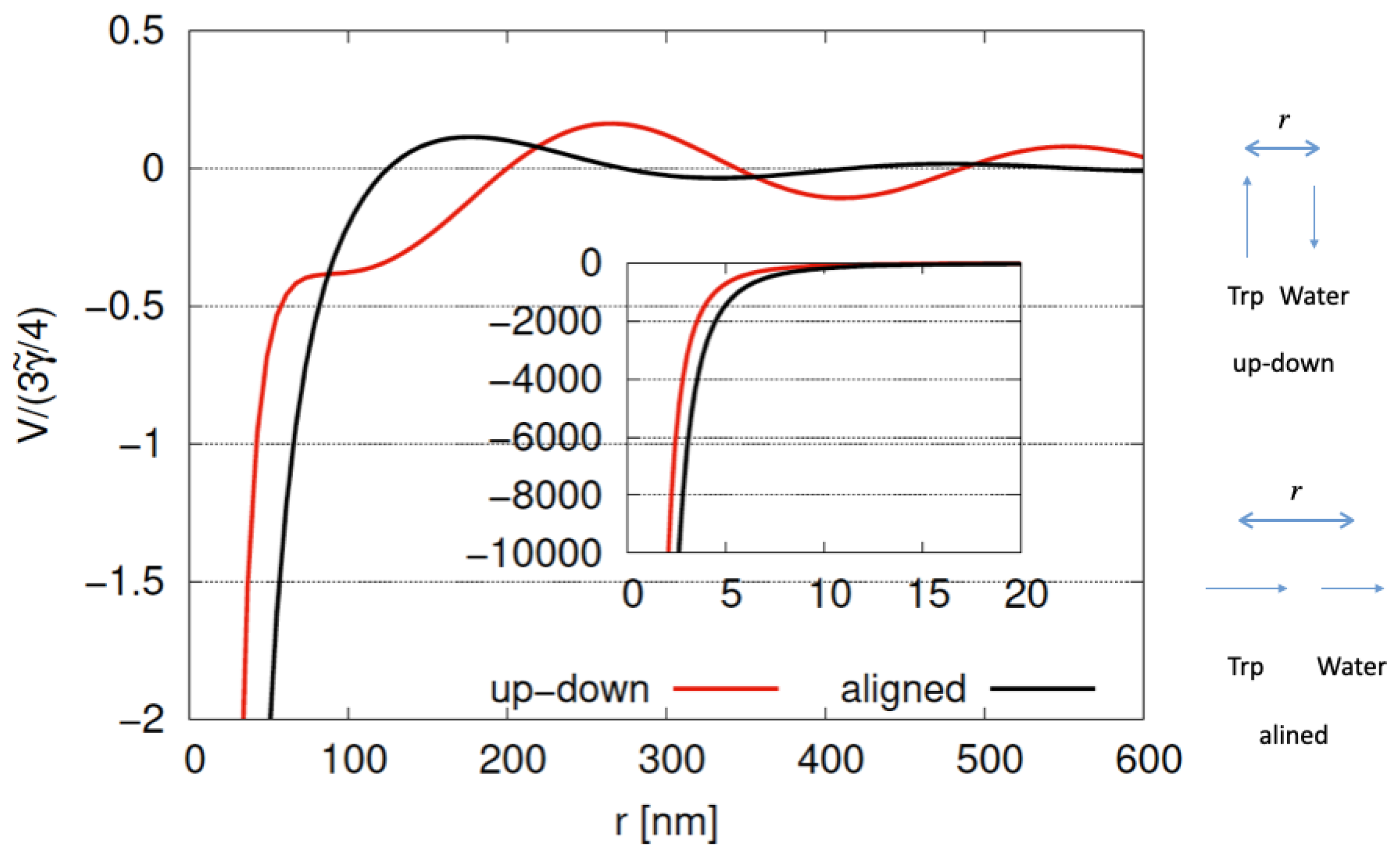
The potential energy (V) between water and tryptophan dipoles [7] is shown in Figure 18 for

$$\begin{array}{ccc}\hfill V\left(r\right)& =& {\displaystyle \frac{3\tilde{\gamma }}{4}}[\left(-{\displaystyle \frac{cos\left(kr\right)}{kr}}+{\displaystyle \frac{sin\left(kr\right)}{{\left(kr\right)}^2}}+{\displaystyle \frac{cos\left(kr\right)}{{\left(kr\right)}^3}}\right){\widehat{\mu }}_{\mathrm{Trp}}·{\widehat{\mu }}_{\mathrm{water}}\hfill \\ & & -\left(-{\displaystyle \frac{cos\left(kr\right)}{\left(kr\right)}}+3{\displaystyle \frac{sin\left(kr\right)}{{\left(kr\right)}^2}}+3{\displaystyle \frac{cos\left(kr\right)}{{\left(kr\right)}^3}}\right)\left({\widehat{\mu }}_{\mathrm{Trp}}·\widehat{r}\right)\left({\widehat{\mu }}_{\mathrm{water}}·\widehat{r}\right),\hfill \end{array}$$

(35)

where r represents the distance between water and tryptophan (Trp) molecules; $k=\omega =4.463 \mathrm{eV}$ represents the energy difference between the ground state and the first excited state; ${\displaystyle \frac{2\pi }{k}}=280 \mathrm{nm}$, ${\widehat{\mu }}_{\mathrm{Trp}}$ and ${\widehat{\mu }}_{\mathrm{water}}$ represent normalized dipole moment vectors for Trp ${\overrightarrow{\mu }}_{\mathrm{Trp}}$ and water molecule ${\overrightarrow{\mu }}_{\mathrm{water}}$, respectively; $\widehat{r}$ represents the normalized relative coordinate between Trp and water given by $\overrightarrow{r}$; and $\tilde{\gamma }$ is $\tilde{\gamma }={\displaystyle \frac{4}{3}}{\displaystyle \frac{k^3}{{ϵ}_r}}|{\overrightarrow{\mu }}_{\mathrm{Trp}}||{\overrightarrow{\mu }}_{\mathrm{water}}|$ (with relative permittivity ${ϵ}_r$) representing $\tilde{\gamma }=3\times {10}^{-7} \mathrm{eV}$. We show cases of an up–down configuration and an aligned configuration for Trp and water dipoles in Figure 18. As shown in Figure 18, we find a large decrease in potential energy for both up–down and aligned configurations, representing large attractive forces between dipoles. For $r<80 \mathrm{nm}$, the potential energy for the aligned configuration is lower than that for the up–down configuration. As r increases, potential energy gradually approaches zero with a wavelength of $280 \mathrm{nm}$ but still showing long-range interaction ($\sim {\displaystyle \frac{1}{r}}$). Long-range interaction might play the role of collective behaviors of Trp and water systems for large scales of microtubules. Trapped water molecules for Trp have been studied in several experimental and theoretical studies. Tryptophans with trapped protonated water molecules (TrpH⁺(H₂O)₃ and TrpH⁺(H₂O)₅) were investigated using cold-ion spectroscopy [35]. The dielectric property of water molecules trapped in tryptophan residue depending on pH was shown in fluorescence emission spectra [36]. Trapped water molecules around tryptophans are key factors of protein fluorescence, since the intrinsic fluorescence of tryptophans is sensitive to the environment surrounding solvents or amino acids [37,38]. In cases in which Trp molecules attract surrounding water molecules and their distances are at atomic scales or extremely small compared with a wavelength of $280 \mathrm{nm}$, quantum effects, such as entanglement, superposition and so on, might emerge. Microtubules involving tryptophans have been shown to be effective light harvesters [5,6]. Aromatic residues, such as tryptophans and tyrosines, might be adopted for information processing roles. Therefore, we need quantum models to describe the fluorescence of tryptophans with surrounding water molecules. Such models might be applied to describe the quantum information processing of tryptophans.

We consider super-radiant and sub-radiant states for two qubits ($j=1,2$) with a decay rate of ${\gamma }_j$. We investigate the following decay matrix ($\mathbf{G}$) appearing on the right-hand side in Equation (16) as follows:

$$\begin{array}{ccc}\hfill \mathbf{G}& =& \left(\begin{array}{cc}{\gamma }_1& \sqrt{{\gamma }_1{\gamma }_2}\\ \sqrt{{\gamma }_1{\gamma }_2}& {\gamma }_2\end{array}\right).\hfill \end{array}$$

(36)

We then find two eigenstates as follows:

$$\begin{array}{ccc}\hfill \mathbf{G}\left(\begin{array}{c}\sqrt{{\gamma }_1}\\ \sqrt{{\gamma }_2}\end{array}\right)& =& ({\gamma }_1+{\gamma }_2)\left(\begin{array}{c}\sqrt{{\gamma }_1}\\ \sqrt{{\gamma }_2}\end{array}\right),\hfill \end{array}$$

(37)

$$\begin{array}{ccc}\hfill \mathbf{G}\left(\begin{array}{c}\sqrt{{\gamma }_2}\\ -\sqrt{{\gamma }_1}\end{array}\right)& =& 0·\left(\begin{array}{c}\sqrt{{\gamma }_2}\\ -\sqrt{{\gamma }_1}\end{array}\right).\hfill \end{array}$$

(38)

The eigenstate expressed as ${(\sqrt{{\gamma }_1},\sqrt{{\gamma }_2})}^t\sim {\displaystyle \frac{\sqrt{{\gamma }_1}{\sigma }_1^{†}|v\rangle +\sqrt{{\gamma }_2}{\sigma }_2^{†}|v\rangle }{\sqrt{{\gamma }_1+{\gamma }_2}}}$ represents a super-radiant state with a large decay rate $({\gamma }_1+{\gamma }_2)$. On the other hand, the eigenstate expressed as ${(\sqrt{{\gamma }_2},-\sqrt{{\gamma }_1})}^t\sim {\displaystyle \frac{\sqrt{{\gamma }_2}{\sigma }_1^{†}|v\rangle -\sqrt{{\gamma }_1}{\sigma }_2^{†}|v\rangle }{\sqrt{{\gamma }_1+{\gamma }_2}}}$ represents a sub-radiant state with a decay rate of 0. In the case of ${\gamma }_1={\gamma }_2$, this sub-radiant state corresponds to $(|10\rangle -|01\rangle )/\sqrt{2}$, representing a spin-0 state of two spin particles ($1/2$). The sub-radiant state is decoupled from spin-1 states, namely $|11\rangle$, $(|10\rangle +|01\rangle )/\sqrt{2}$ and $|00\rangle$, corresponding to intermediate states in a decaying processes for super-radiant states. Let us now increase the ratio ${\gamma }_2/{\gamma }_1$ from 1. In the case of ${\gamma }_2/{\gamma }_1\gg 1$, the sub-radiant state (${\displaystyle \frac{\sqrt{{\gamma }_2}{\sigma }_1^{†}|v\rangle -\sqrt{{\gamma }_1}{\sigma }_2^{†}|v\rangle }{\sqrt{{\gamma }_1+{\gamma }_2}}}$) is approximately ${\sigma }_1^{†}|v\rangle =|10\rangle$. As a result, the state of $|10\rangle$ for qubit 1 coupled with qubit 2 with an extremely large decay rate of ${\gamma }_2/{\gamma }_1\gg 1$ is stable over the course of time evolution. We propose the adoption of sub-radiance to achieve robustness of data qubits of tryptophans entangled with JQFs of water molecules. Our approach to maintain quantum information is distinguished from making use of quantum Zeno effects involving continuous measurement procedures [39]. We adopt the time evolution of expectation values of operators based on Heisenberg equations. Then no measurement procedures are necessary. We prepare two qubits with decay rates of ${\gamma }_1$ and ${\gamma }_2$. Quantum entanglement between two qubits then suggests a super-radiant state with a decay rate of ${\gamma }_1+{\gamma }_2$ and sub-radiant state with a vanishing decay rate in a Heisenberg equation with a total decay rate of ${\gamma }_1+{\gamma }_2$ remaining. We can then use sub-radiance with a vanishing decay rate for data qubits.

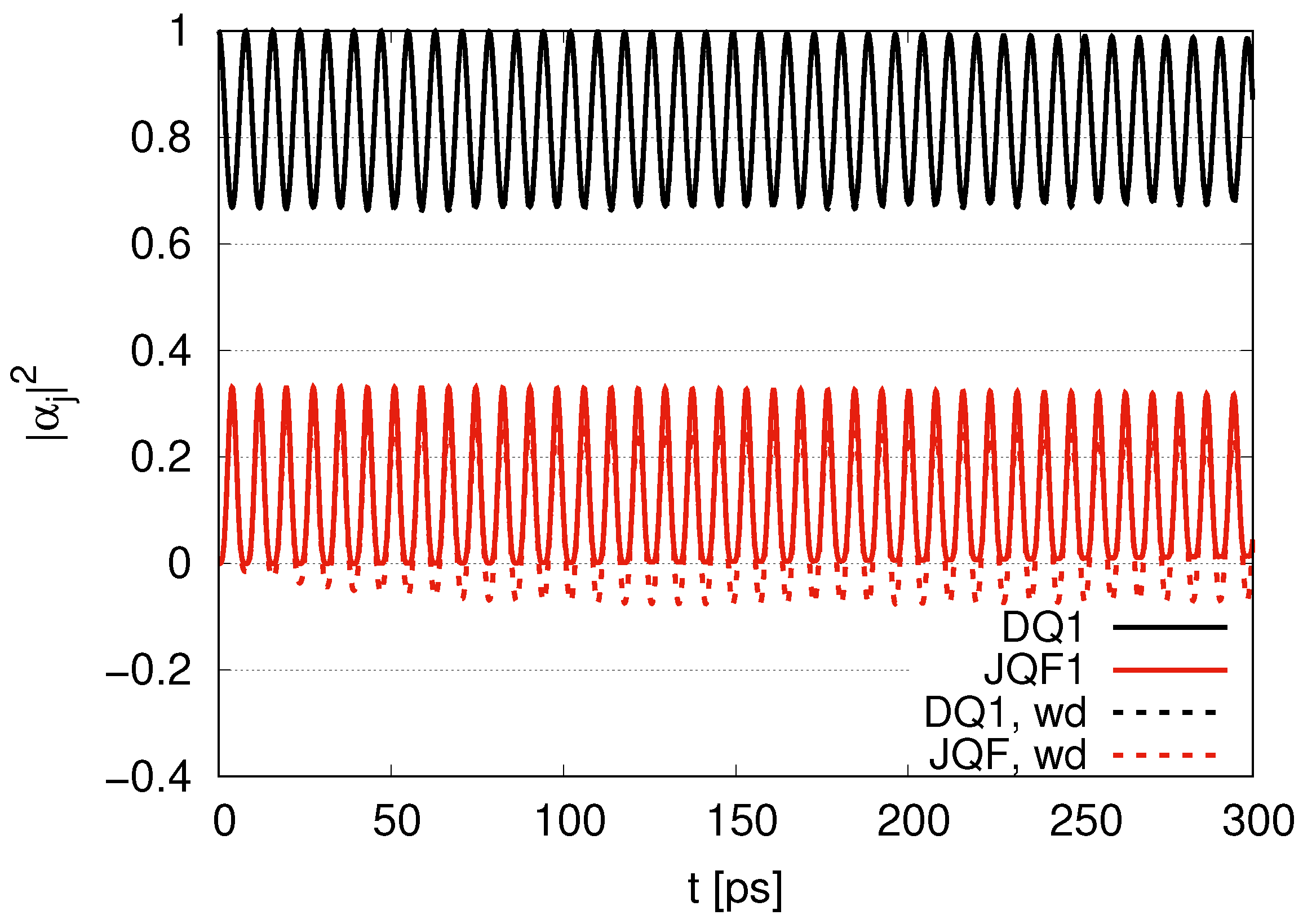
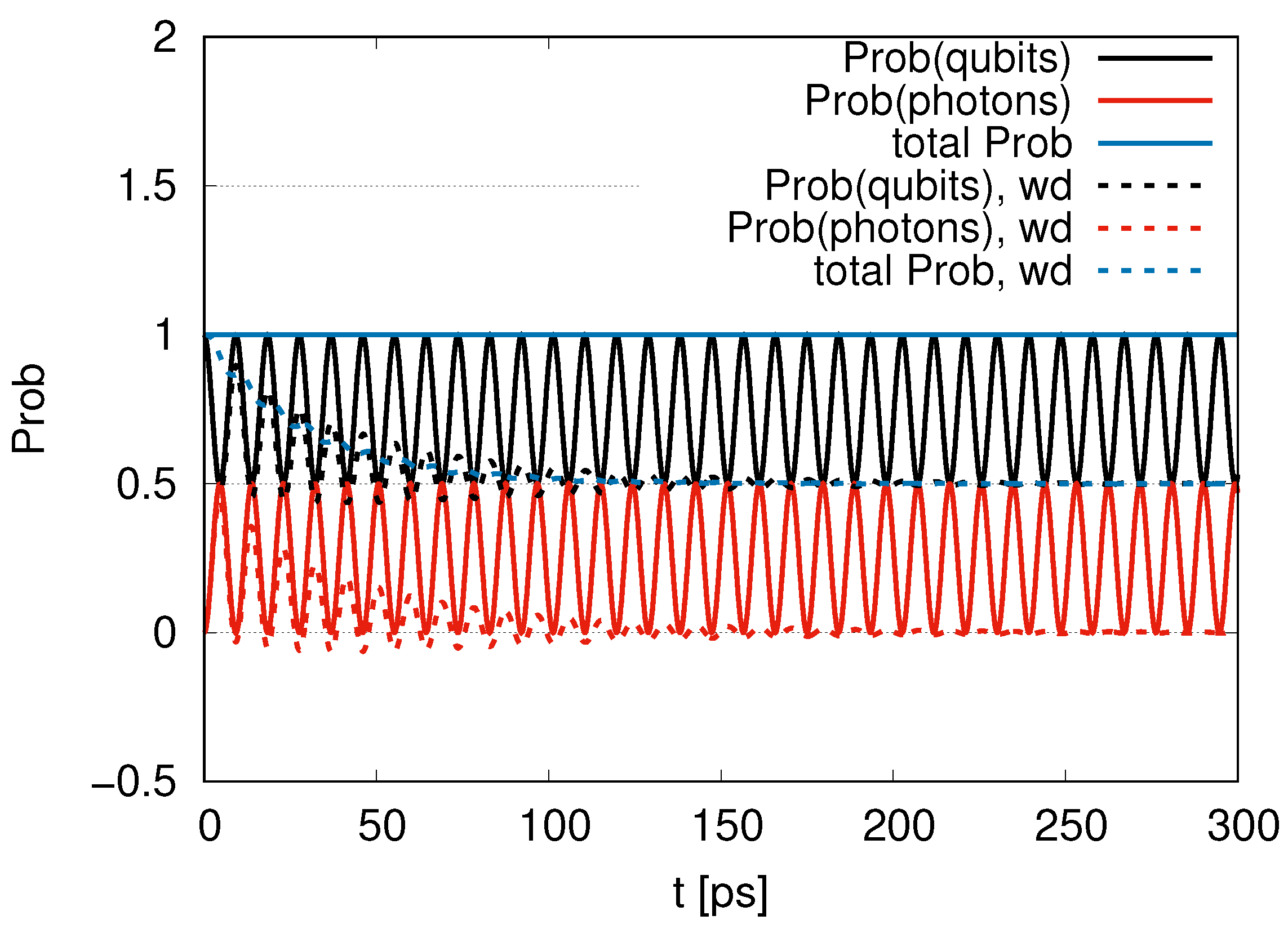
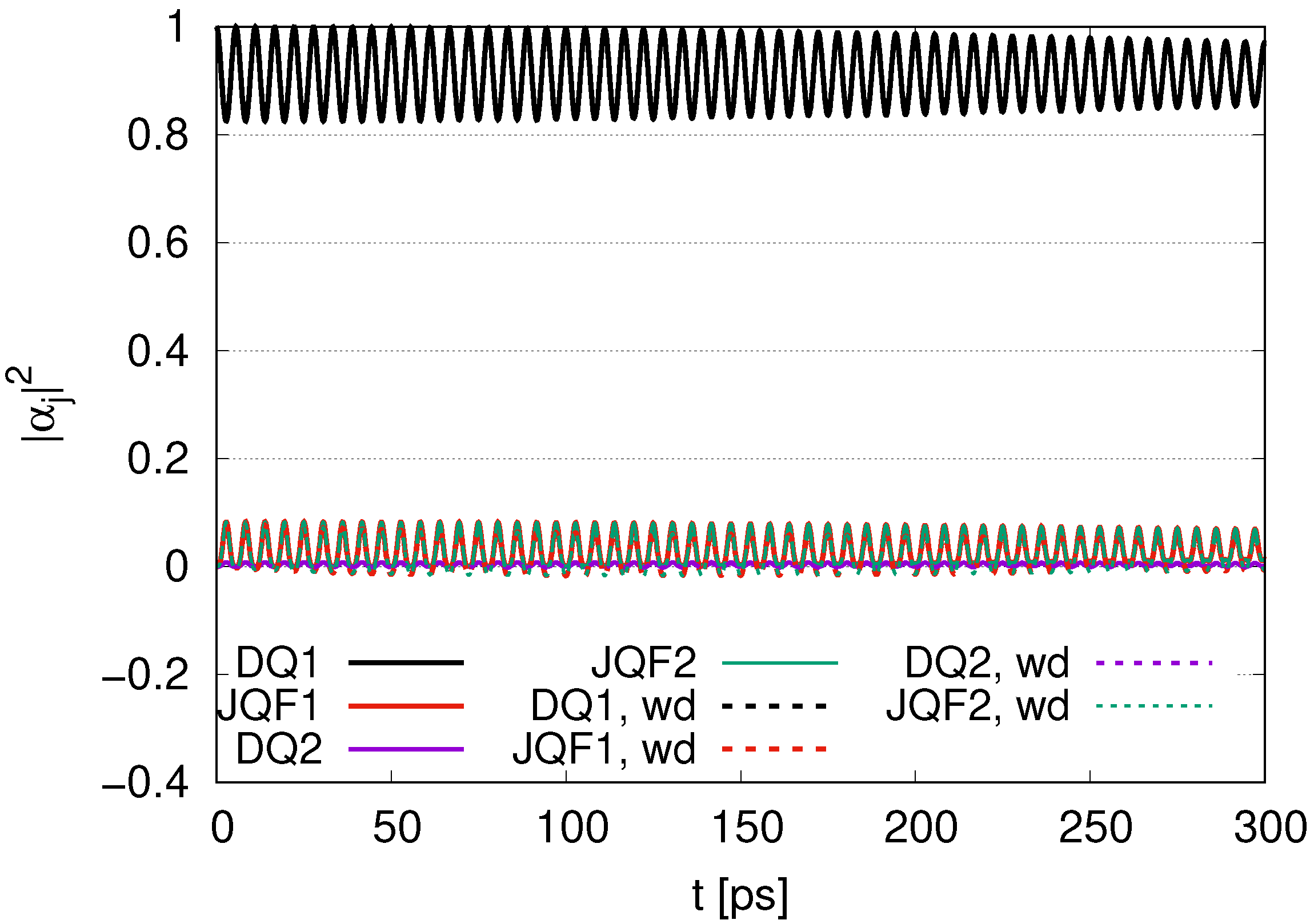
Sub-radiance emerging with an increasing ratio is shown in Section 3.1, where we introduced two qubits (one DQ and one JQF) in the same position ($r_j=0$). For the ratio of the decay rates (${\gamma }_{\mathrm{JQF}}/{\gamma }_{\mathrm{DQ}}=1$) in Figure 2, we find an interplay of probability between DQ and JQF. There is no distinction between DQ and JQF. In the case of a ratio 10, as shown in Figure 3, the average values of $|{\alpha }_j{|}^2$ for DQ and JQF are 0.83 and 0.17, respectively. Here, determine the ratio to be $0.83/0.17=4.9$. 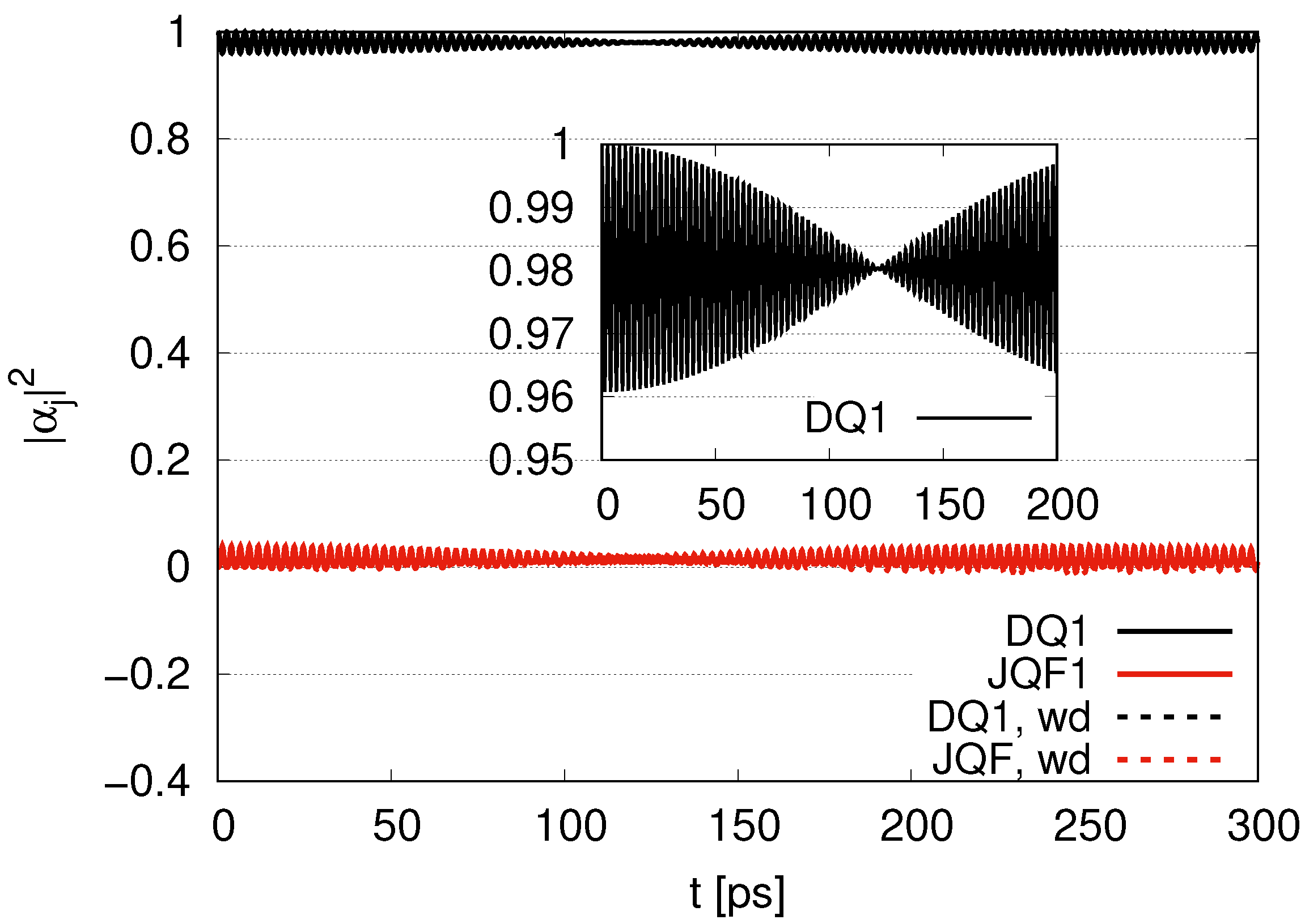Since the ratio of the decay rates is 10, the ratio 4.9 is roughly one half of 10. This is because part of the excitation of DQ is transferred to photon modes. In the case of a ratio 100, as shown in Figure 4, the average values of $|{\alpha }_j{|}^2$ for DQ and JQF are 0.98 and 0.02, respectively. We find a ratio $0.98/0.02=49$ and that the order is half of 100 due to contributions of the excitation of photons. As we increase the ratio of decay rates for DQ and JQF, the $|{\alpha }_j{|}^2$ for DQ remains around the initial value of 1. For a ratio 100, the corresponding time scales are $1/{\gamma }_{\mathrm{DQ}}=1.9 \mathrm{ns}$ and $1/{\gamma }_{\mathrm{JQF}}=19 \mathrm{ps}$, which might correspond to the time scales of internal losses and are 20 times larger than thermalization time scales ($\sim 1 \mathrm{ps}$) for water–photon systems where we set the mean free path of water molecules to $0.13 \mathrm{nm}$ and the mean velocity of water molecules to $\mathrm{600}\mathrm{m}·{\mathrm{s}}^{-1}$, finding $4\times 0.13 \mathrm{nm}/600\mathrm{m}·{\mathrm{s}}^{-1}=1 \mathrm{ps}$ with four collision processes.

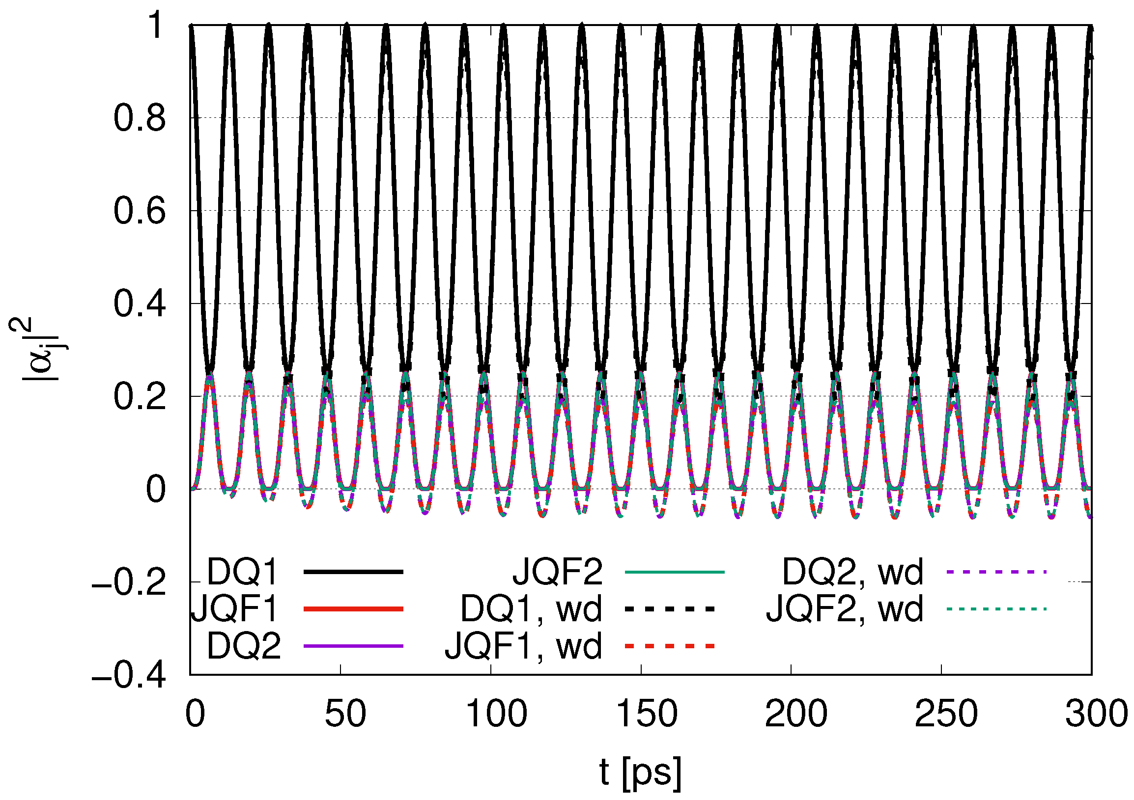
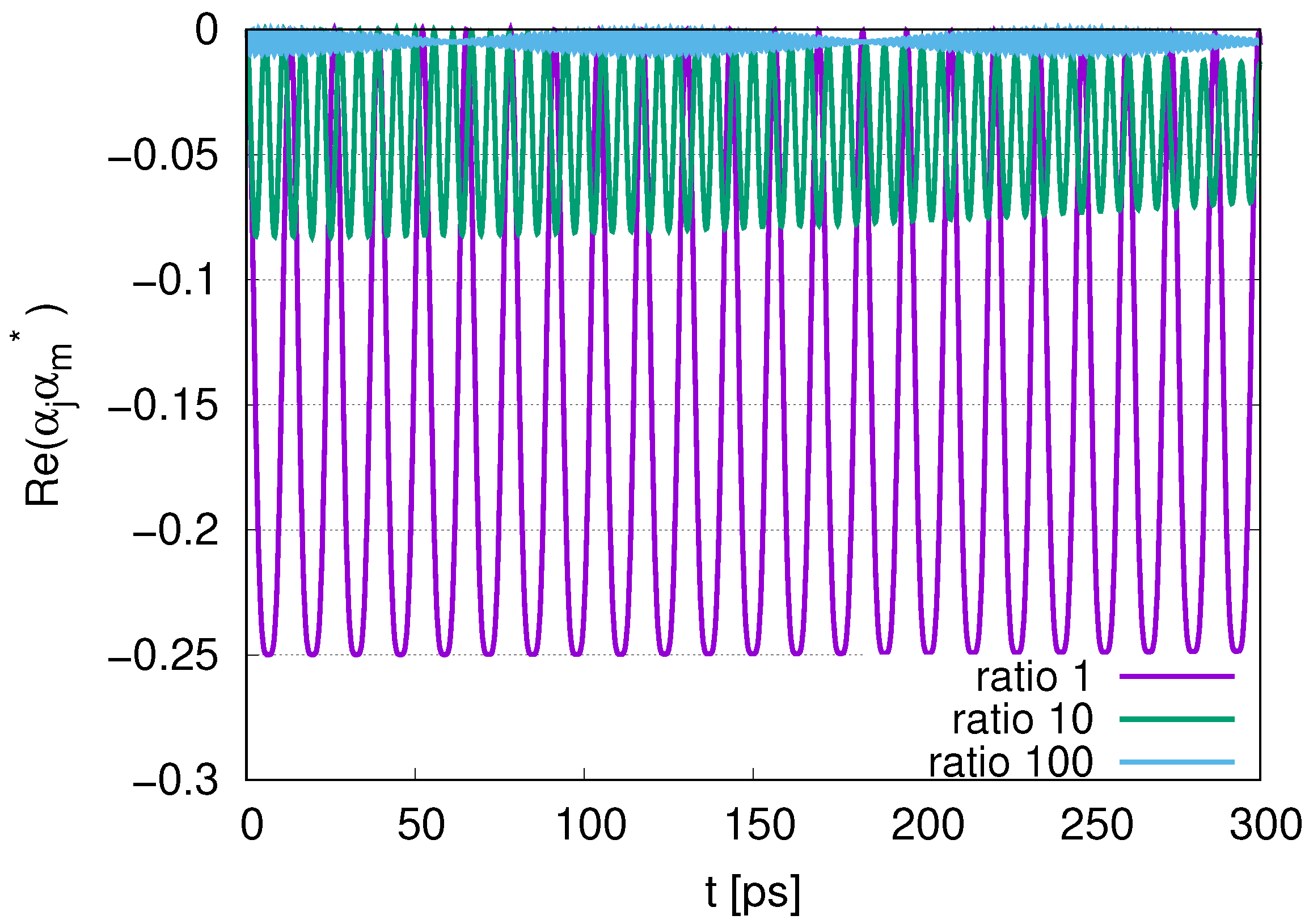
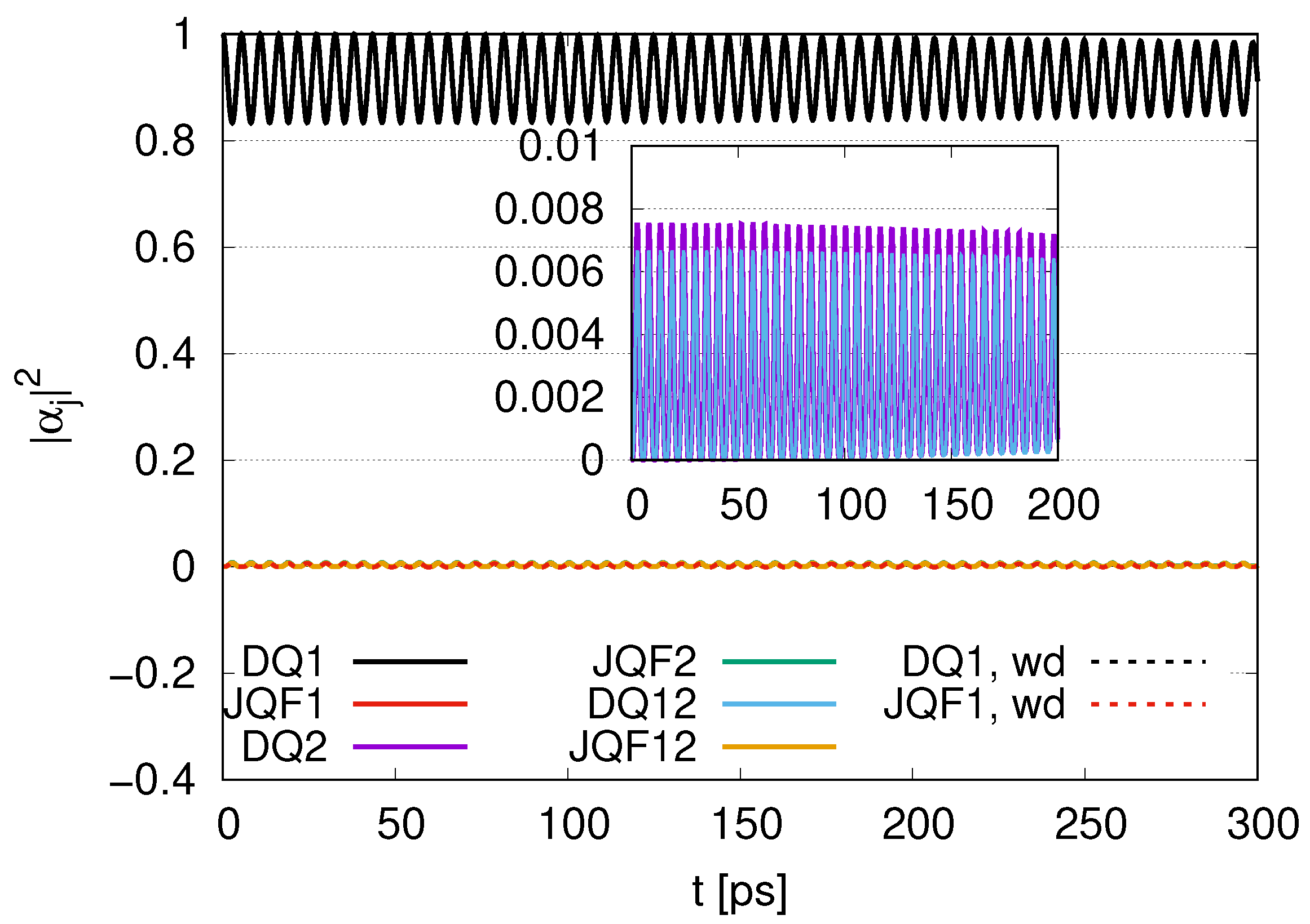
The other type of sub-radiance for a ratio 1 involving 4 and 24 qubits is shown in Figure 8 and Figure 14. Even if the ratio is 1, we find that $|{\alpha }_j{|}^2$ for DQ1 oscillates between 0.25 and 1, as shown in Figure 8. We infer that the other type of the sub-radiant state ($3{\sigma }_{\mathrm{DQ}1}^{†}|v\rangle -{\sigma }_{\mathrm{DQ}2}^{†}|v\rangle -{\sum }_{j=\mathrm{JQF}1}^{\mathrm{JQF}2}{\sigma }_j^{†}|v\rangle$) appears since Re ${\alpha }_j{\alpha }_m^{*}$ with $j=$ DQ1 and $m=$ DQ2 has negative values between $-0.25$ and 0, as shown in Figure 11. The ratio of coefficients for DQ1 and DQ2 is $3^2/1^2=9$, while the ratio of the average of $|{\alpha }_j{|}^2$ for DQ1 and $|{\alpha }_j{|}^2$ for DQ2 is $0.62/0.12=5.2$, which is smaller than 9 because excitations of qubits are transferred to photon excitations. Similarly, we also infer that the sub-radiant state ($23{\sigma }_{\mathrm{DQ}1}^{†}|v\rangle -{\sum }_{j=\mathrm{DQ}2}^{\mathrm{DQ}12}{\sigma }_j^{†}|v\rangle -{\sum }_{j=\mathrm{JQF}1}^{\mathrm{JQF}12}{\sigma }_j^{†}|v\rangle$) appears. The ratio of the coefficients for DQ1 and other qubits is ${23}^2=529$, while the ratio of the averages of $|{\alpha }_j{|}^2$ for DQ1 and $|{\alpha }_j{|}^2$ for DQ2 is $0.92/0.0075=123$. The ratio of $|{\alpha }_j{|}^2$ for DQ1 and $|{\alpha }_j{|}^2$ for DQ12 is $0.92/0.0067=137$, approaching the order of 529. The initial state of DQ1 is protected by other surrounding qubits under this type of sub-radiance. However, comparing it with the sub-radiance in making use of the different decay rates for DQ and JQF, the deviation of $|{\alpha }_j{|}^2$ for DQ1 from its initial value 1 is dependent on the number of surrounding qubits, which means that we should use more surrounding qubits for the stability of data. This represents the waste of resources in terms of qubits. Making use of surrounding water molecules with larger decay rates than JQFs might be more advantageous in protecting data contained in a microtubule.

The temperature dependence is extremely low in the course of the time evolution of qubits. This is because $\omega =4.463 \mathrm{eV}$ for tryptophan is extremely large compared with a temperature of $T=310 \mathrm{K}=27 \mathrm{meV}$. Although we investigated several temperatures ($200 \mathrm{K}$, $310 \mathrm{K}$ and $400 \mathrm{K}$) for a total of two qubits, when the ratio of decay rates of DQ and JQF is 10, there are minimal changes in $|{\alpha }_j{|}^2$ for DQ1. As the temperature approaches the order of $\omega$, the amplitudes of oscillations of $|{\alpha }_j{|}^2$ gradually increase.

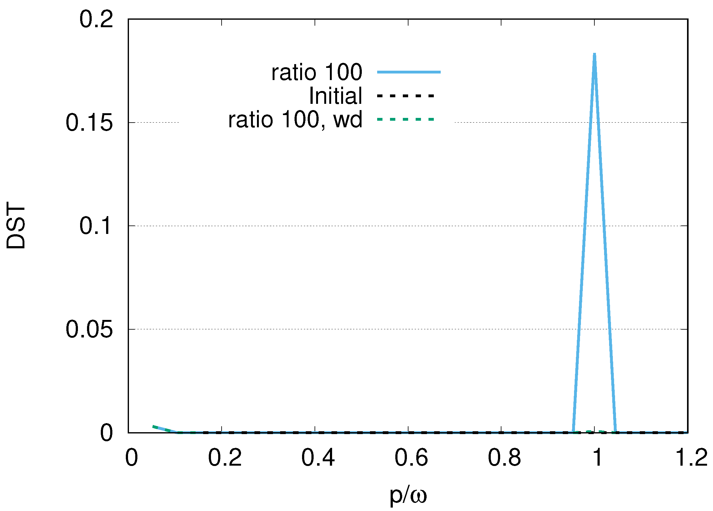
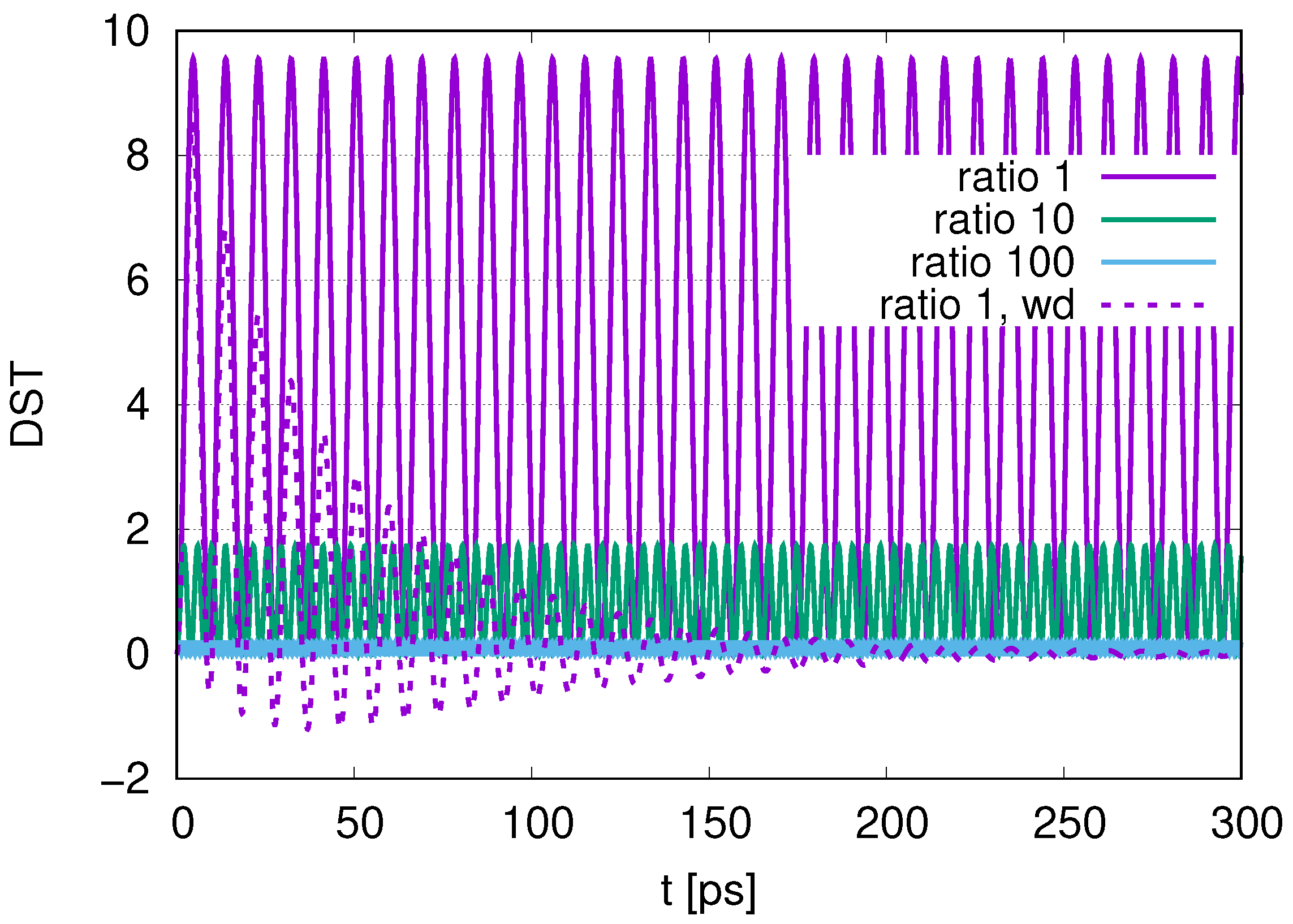
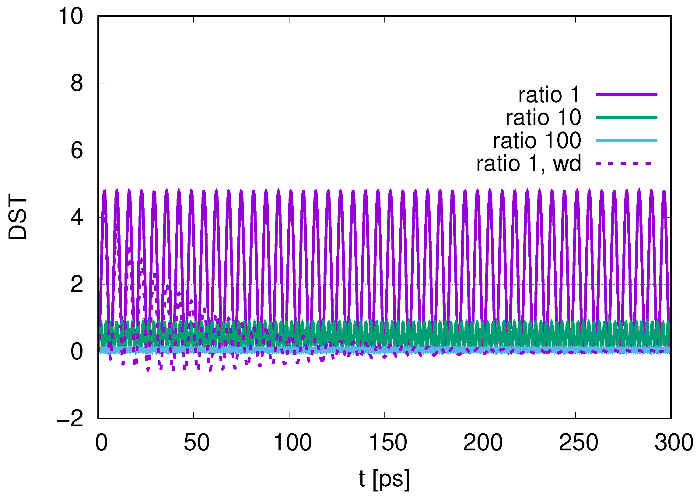
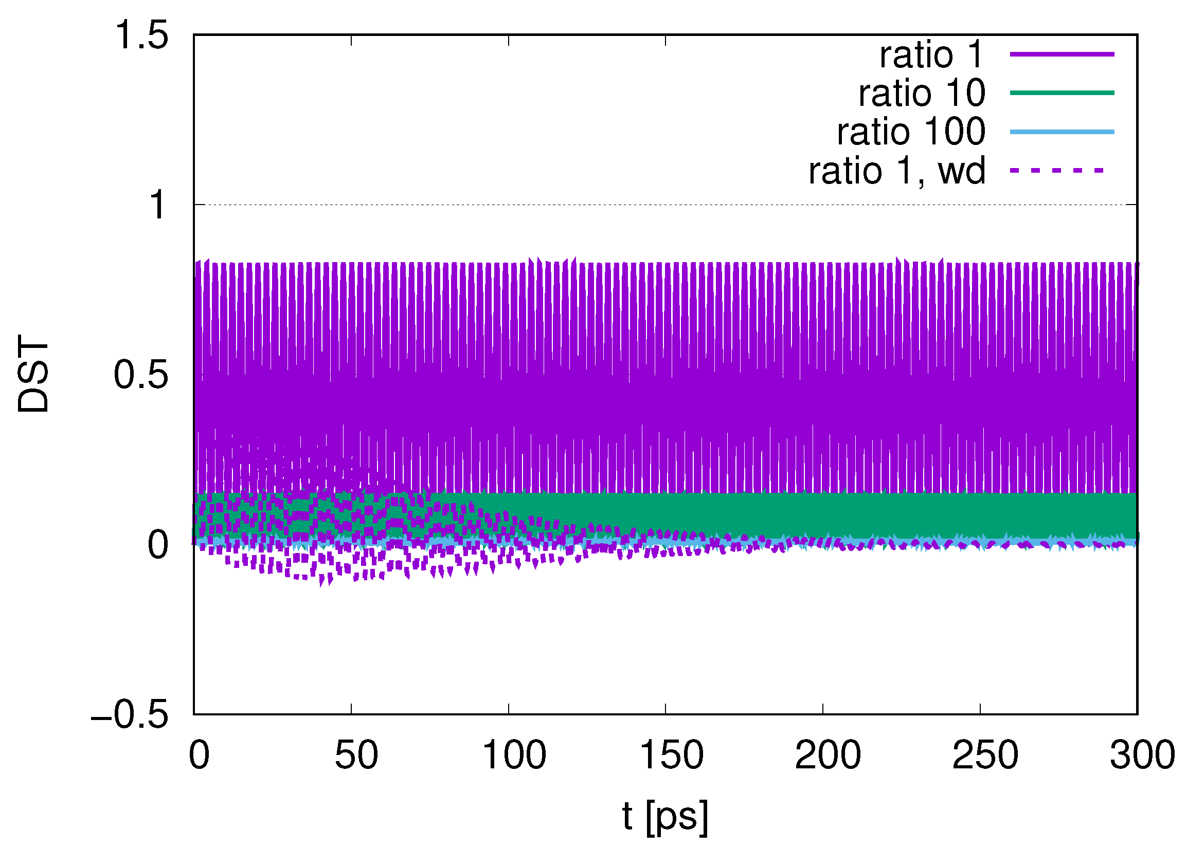
In this paper, we adopted wQED with several photon modes. As shown in Figure 5, the contribution of photon modes is almost only the resonant mode ($p/\omega =1$) at a temperature of $310 \mathrm{K}$. As we increase the number of DQs in Figure 6, Figure 12 and Figure 17, the maximum values in the distribution of the peak of photon modes (DST) decrease in the course of time evolution. We also find that as we increase the ratio of the decay rates, the maximum values of DST decrease, with smaller leakage to the excitations of photons, which reflects the merit of adopting sub-radiance with robust states of qubits.

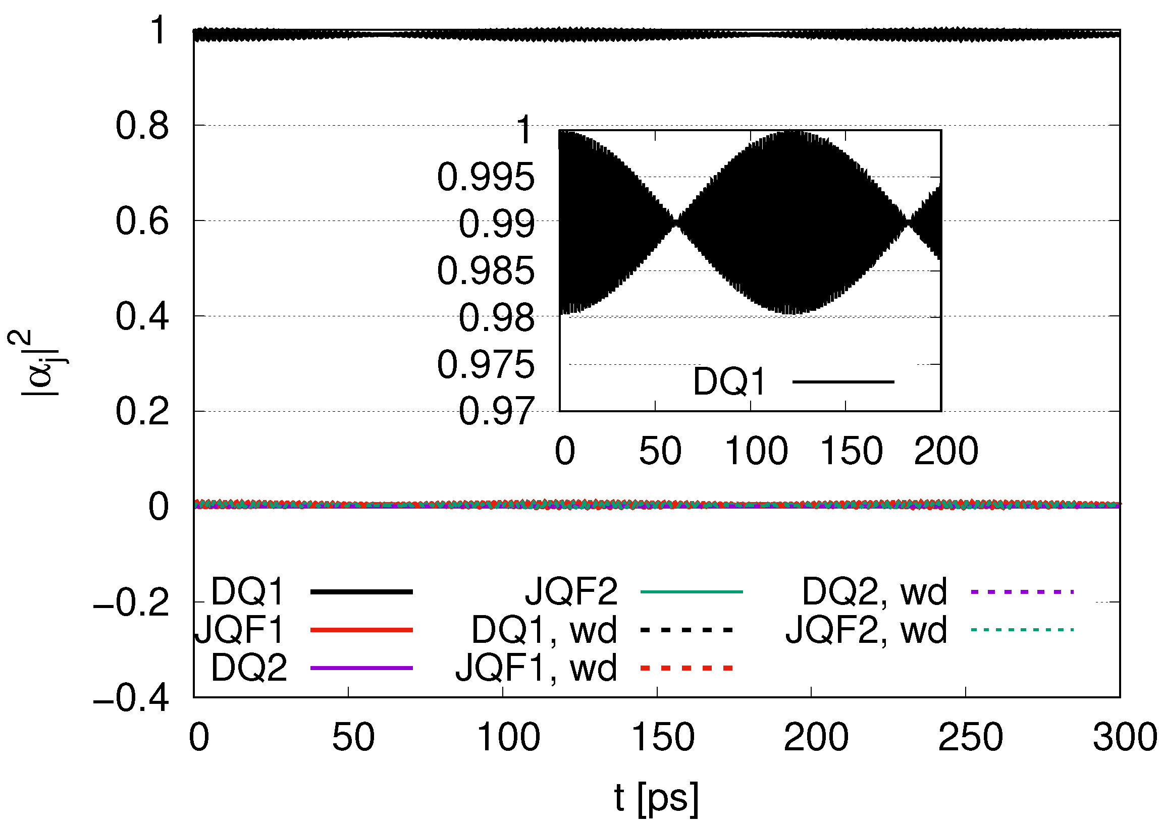
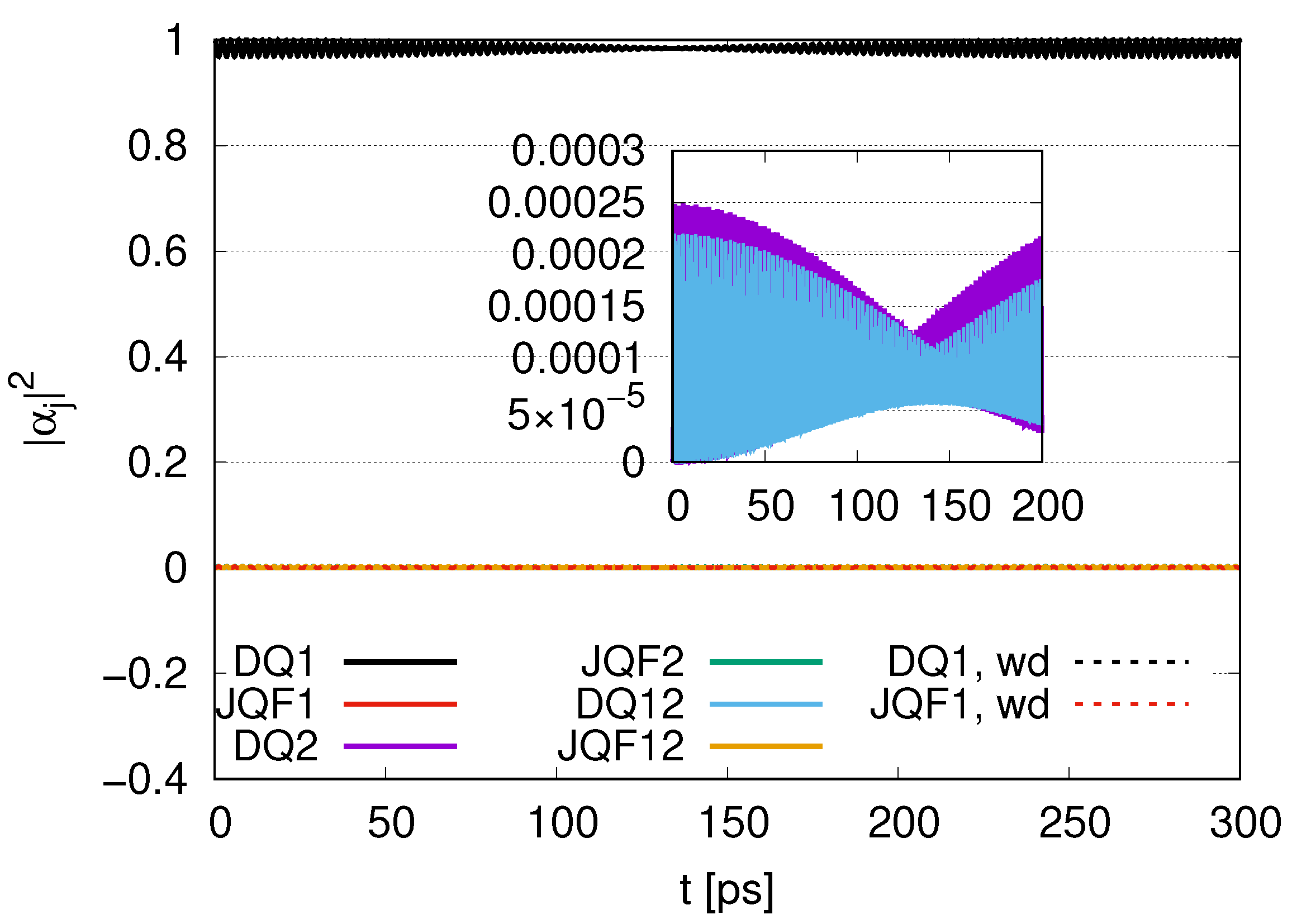
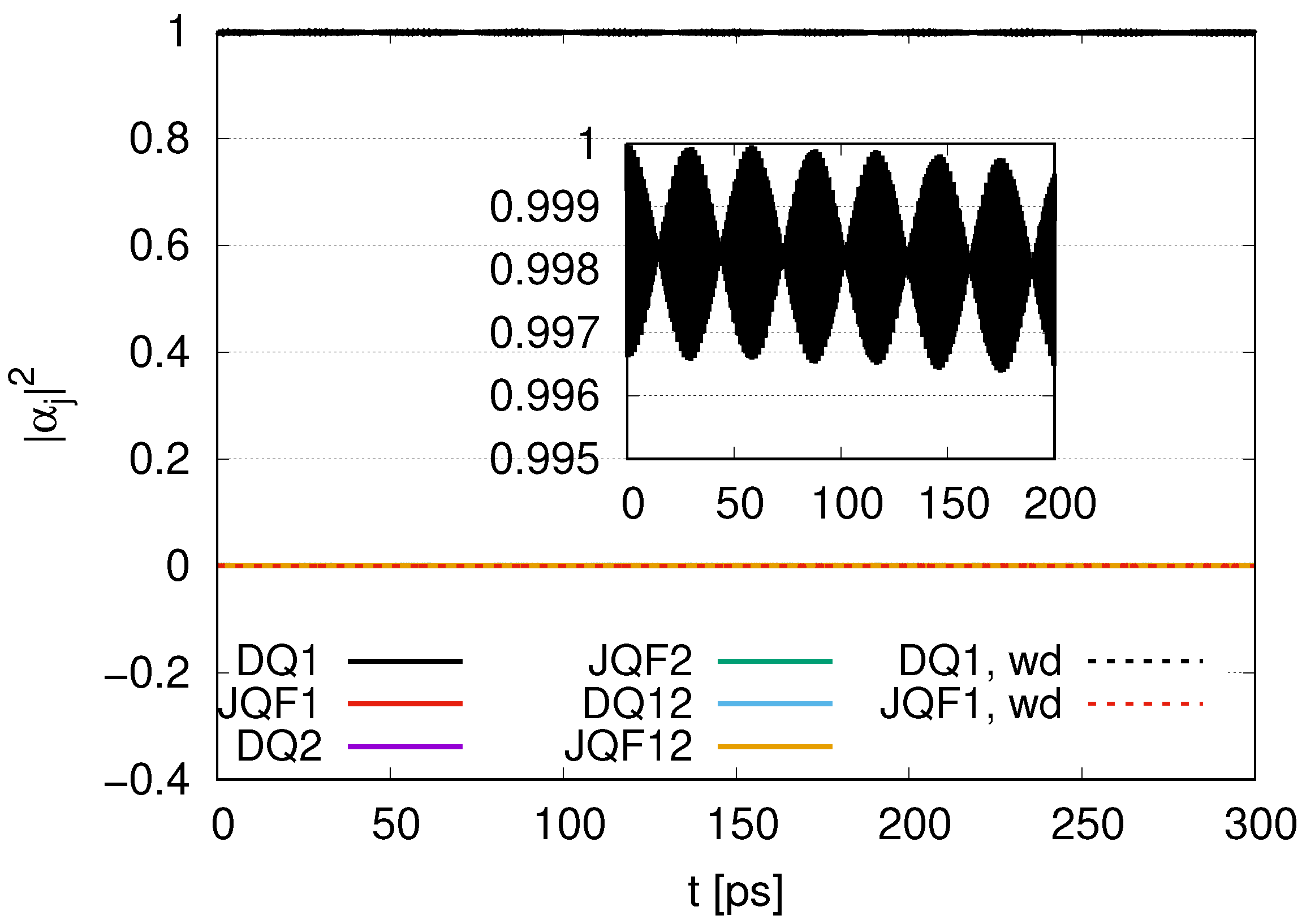
We can compare $|{\alpha }_j{|}^2$ with the ratio 100 for 1 DQ in Figure 4, for 2 DQs in Figure 10 and for 12 DQs in Figure 16. As the number of DQs increases, the $|{\alpha }_j{|}^2$ for DQ1 tends to approach the initial value of 1 in the course of time evolution, with an average of 0.98 in Figure 4, 0.99 in Figure 10 and 0.998 in Figure 16. In addition, the average of $|{\alpha }_j{|}^2$ for JQF1 in Figure 4 is 0.02, that of JQF2 in Figure 10 is 0.005 and that of JQF12 in Figure 16 is 0.00013. The ratios of the averages of $|{\alpha }_j{|}^2$ for DQ1 and JQF are

$$\begin{array}{c}\hfill {\displaystyle \frac{0.98}{0.02}}:{\displaystyle \frac{0.99}{0.005}}:{\displaystyle \frac{0.998}{0.00013}}=50:200:7700=1:4:150.\end{array}$$

(39)

We can conclude that sub-radiant states are realized as $\sqrt{{\gamma }_{\mathrm{JQF}}}{\sigma }_{\mathrm{DQ}1}^{†}|v\rangle -\sqrt{{\gamma }_{\mathrm{DQ}}}{\sigma }_{\mathrm{JQF}1}^{†}|v\rangle$ for the case of 1 DQ, $2\sqrt{{\gamma }_{\mathrm{JQF}}}{\sigma }_{\mathrm{DQ}1}^{†}|v\rangle -\sqrt{{\gamma }_{\mathrm{DQ}}}{\sum }_{j=\mathrm{JQF}1}^{\mathrm{JQF}2}{\sigma }_j^{†}|v\rangle$ for the case of 2 DQs and $12\sqrt{{\gamma }_{\mathrm{JQF}}}{\sigma }_{\mathrm{DQ}1}^{†}|v\rangle -\sqrt{{\gamma }_{\mathrm{DQ}}}{\sum }_{j=\mathrm{JQF}1}^{\mathrm{JQF}12}{\sigma }_j^{†}|v\rangle$ for the case of 12 DQs. We now calculate the ratio of $|{\alpha }_j{|}^2$ for DQ1 and JQF. We find

$$\begin{array}{c}\hfill {\left({\displaystyle \frac{\sqrt{{\gamma }_{\mathrm{JQF}}}}{\sqrt{{\gamma }_{\mathrm{DQ}}}}}\right)}^2:{\left({\displaystyle \frac{2\sqrt{{\gamma }_{\mathrm{JQF}}}}{\sqrt{{\gamma }_{\mathrm{DQ}}}}}\right)}^2:{\left({\displaystyle \frac{12\sqrt{{\gamma }_{\mathrm{JQF}}}}{\sqrt{{\gamma }_{\mathrm{DQ}}}}}\right)}^2=1:4:144,\end{array}$$

(40)

for the cases of 1 DQ, 2 DQs and 12 DQs, respectively. The numerical results shown in Equation (39) correspond to those for the sub-radiant states in Equation (40).

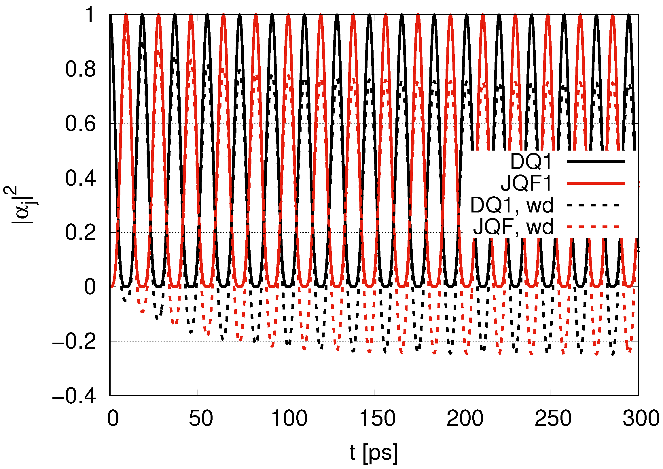
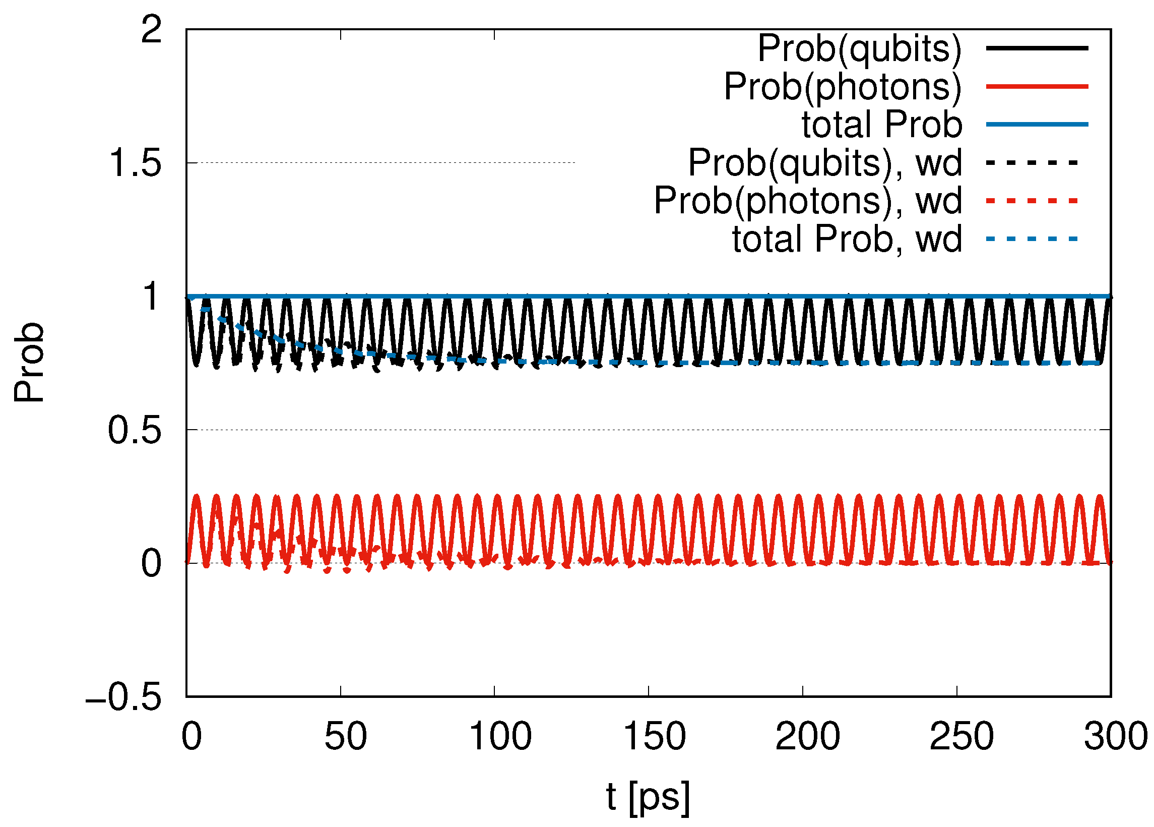
We have described the damping processes of photon modes in Equation (29) by changing $\Gamma /\omega =0$ to $\Gamma /\omega =1\times {10}^{-5}$. We find that the damping affects the average of $|{\alpha }_j{|}^2$ in the cases of a ratio 1 in Figure 2 and Figure 8. We also find convergence to the initial values for photon modes in Figure 6 and Figure 12. As we increase the ratio of the decay rate (${\gamma }_{\mathrm{JQF}}/{\gamma }_{\mathrm{DQ}}$) to 10, then to 100 in Figure 3 and Figure 4, respectively, the effects of damping tend to disappear over time evolution. This is because $|{\alpha }_j{|}^2$ for DQ1 is nearly equal to 1, and the absolute values of the distribution of photon modes cease to increase, as shown in Figure 6 and Figure 12. Adopting the sub-radiant states, little changes occur due to the damping of photon modes that appear in time evolution.

We should also discuss the extension of our model to three-dimensional cases. In this paper, we considered a one-dimensional waveguide QED for the model of tryptophans in tubulin dimers. To extend this to a three-dimensional case, we extend ${\xi }_{jk}$ in Equation (3) to ${\xi }_{j\mathbf{k}}=\sqrt{{\displaystyle \frac{{\gamma }_j}{\pi }}}cos\left(\mathbf{k}·{\mathbf{r}}_j+\theta \right)$ with three-dimensional momenta $\mathbf{k}$ for the photon modes and position ${\mathbf{r}}_j$ for the jth qubit. Even if we extend our model to a thee-dimensional case, since we can estimate $\mathbf{k}·{\mathbf{r}}_j\sim \omega |{\mathbf{r}}_j|\sim 4.463 \mathrm{eV}\times 1.333 \mathrm{nm}\times 11\sim 0.03016\times 11<{\displaystyle \frac{\pi }{2}}$ for 12 DQs in two tubulin dimers, little change is expected to appear in the course of time evolution.

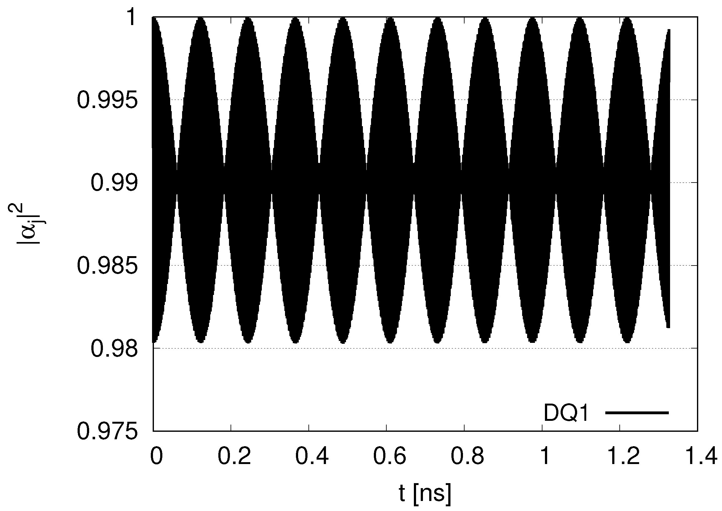
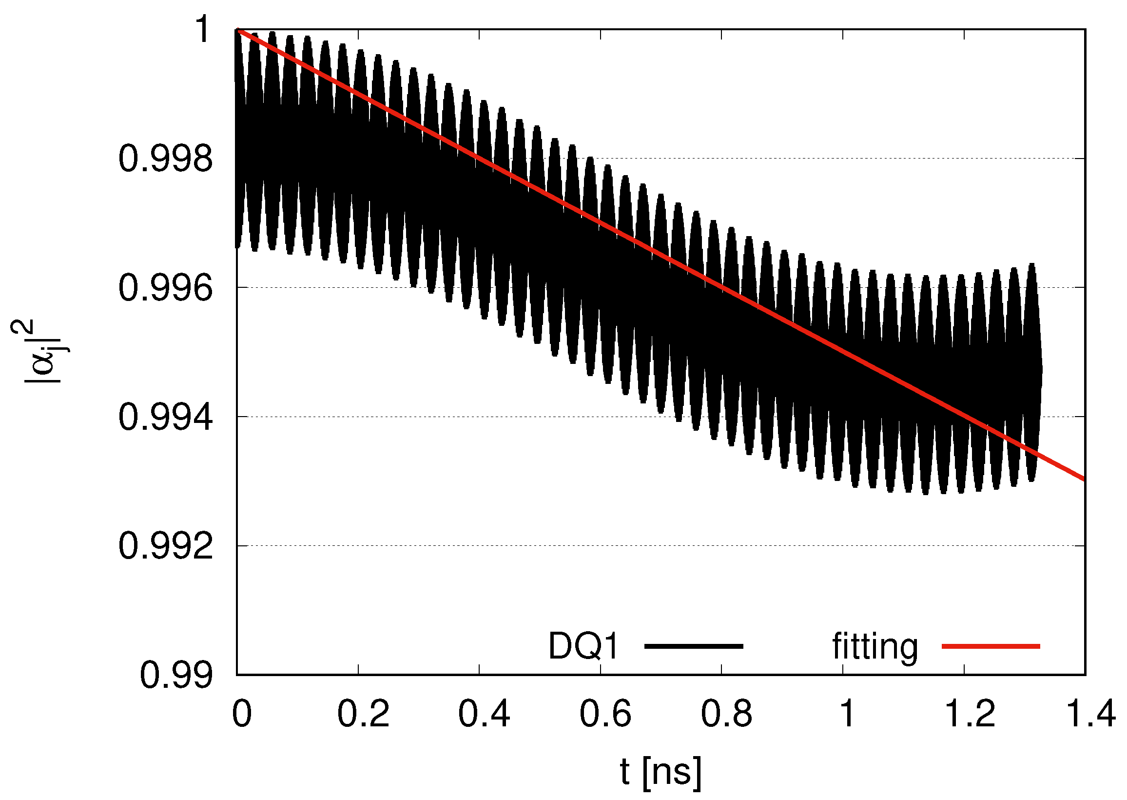
Longer simulations are shown in Appendix A. In the case of two DQs and two JQFs in Figure A1, little decay for $|{\alpha }_j{|}^2$ appears for DQ1 at $t<1.3 \mathrm{ns}$. On the other hand, in the case of 12 DQs and 12 JQFs in Figure A2, we find a slight decay of fitting $exp\left(-{\displaystyle \frac{t}{\tau }}\right)$ with $\tau =200 \mathrm{ns}$, although the decrease seems to be moderate at $t\sim 1 \mathrm{ns}$. We can consider the size of the system to discuss the decay. In the case of 2 DQs and 2 JQFs, the size of the system is $8/6\times 2\sim 3 \mathrm{nm}$, while the size is $16 \mathrm{nm}$ in the case of 12 DQs and 12 JQFs. The diffusion length of excitation energy transport in a microtubule was estimated an the experimental study as the order of $6.6 \mathrm{nm}$ [5]. As the size of the system in our simulations increases gradually from $6.6 \mathrm{nm}$, the effects of diffusion might gradually emerge. Although we encounter diffusion effects in maintaining data qubits for larger simulations, quantum entanglement might disappear for distant qubits in microtubules. Since the systems for distant qubits behave independently, the dynamics of the DQs and JQFs might be described by near qubits, as in the case of two DQs and two JQFs. Our experimental study suggests that the fluorescence lifetime of tryptophan is a few ns. Our simulation reported in this paper describes nanosecond scales comparable with the fluorescence lifetime. If we assume a larger decay rate (${\gamma }_{\mathrm{JQF}}$) for JQFs representing water molecules (with a ratio larger than 100), the robustness of data qubits is reinforced. A balance of diffusion and robustness of sub-radiant states is significant.

Maintaining quantum coherence at high temperatures is a demanding task in biological systems. Our strategy is to regard biological systems, especially brains, as open systems. Life is a flow of energy and matter. To maintain biological systems, we prepared three systems, namely an energy supply, physical system and heat bath. We provided continuous energy flow from the energy supply, through the physical system to the heat bath for dissipation of energy. The Fröhlich condensate represents an example suggested in the flow of these three systems, with Bose–Einstein condensate proposed in biological systems [40,41,42]. Self-organization and error corrections due to energy supply represent key concepts for life. We investigated the brain as an open system achieving biological order. In particular, microtubules have an energy source supplied by surrounding mitochondria and heat baths in cells [43,44]. In the case of error corrections by the energy supply to overcome decoherence, quantum coherence might be maintained.

5. Concluding Remarks and Perspectives

The use of waveguide QED for tryptophans in tubulin dimers forming a microtubule as data qubits was the focus of our investigations in this paper. We considered tryptophans to be entangled with water molecules localized in the neighboring positions to those of tryptophan residues in tubular dimers. The use of data qubits for tryptophans has been shown to retain initial states by adopting sub-radiant states entangled with water molecules. Using the robustness of data qubits, we demonstrated the feasibility of quantum information processing that can be performed by tryptophans in a microtubule as local events. If these local events are amplified to non-local events by holographic information processing, the memory localized in a microtubule is diffused throughout the whole brain, and the interplay between data qubits in microtubules and water–photon degrees of freedom in QBD are expected. Our paper presents a formal quantum field theoretic model and its consequences for previously hypothesized processes implicated in quantum mechanisms of cognition at the level of sub-cellular substrates [45,46,47].

References

1. Boisseau, R.P.; Vogel, D.; Dussutour, A. Habituation in non-neural organisms: Evidence from slime moulds. Proc. R. Soc. B Biol. Sci. 2016, 283, 20160446. [Google Scholar] [CrossRef]
2. Craddock, T.J.A.; Tuszynski, J.A.; Hameroff, S. Cytoskeletal Signaling: Is Memory Encoded in Microtubule Lattices by CaMKII Phosphorylation? PLoS Comput. Biol. 2012, 8, e1002421. [Google Scholar] [CrossRef] [PubMed]
3. Murata, M.; Leibnitz, K. Fluctuation-Induced Network Control and Learning: Applying the Yuragi Principle of Brain and Biological Systems; Springer: Singapore, 2021. [Google Scholar]
4. Lee, G.; Leech, G.; Rust, M.J.; Das, M.; McGorty, R.J.; Ross, J.L.; Robertson-Anderson, R.M. Myosin-driven actin-microtubule networks exhibit self-organized contractile dynamics. Sci. Adv. 2021, 7, eabe4334. [Google Scholar] [CrossRef] [PubMed]
5. Kalra, A.P.; Benny, A.; Travis, S.M.; Zizzi, E.A.; Morales-Sanchez, A.; Oblinsky, D.G.; Craddock, T.J.; Hameroff, S.R.; MacIver, M.B.; Tuszynski, J.A.; et al. Electronic energy migration in microtubules. ACS Cent. Sci. 2023, 9, 352–361. [Google Scholar] [CrossRef]
6. Kalra, A.P.; Biswas, S.; Mulrain, I.; Wang, M.; Tuszynski, J.A.; Scholes, G.D. All lit up: Exploring the photophysical properties of protein polymers. J. Phys. Chem. Lett. 2023, 14, 5891–5900. [Google Scholar] [CrossRef] [PubMed]
7. Celardo, G.; Angeli, M.; Craddock, T.; Kurian, P. On the existence of superradiant excitonic states in microtubules. New J. Phys. 2019, 21, 023005. [Google Scholar] [CrossRef]
8. Babcock, N.; Montes-Cabrera, G.; Oberhofer, K.; Chergui, M.; Celardo, G.; Kurian, P. Ultraviolet superradiance from mega-networks of tryptophan in biological architectures. J. Phys. Chem. B 2024, 128, 4035–4046. [Google Scholar] [CrossRef]
9. Kim, J.H.; Aghaeimeibodi, S.; Richardson, C.J.; Leavitt, R.P.; Waks, E. Super-radiant emission from quantum dots in a nanophotonic waveguide. Nano Lett. 2018, 18, 4734–4740. [Google Scholar] [CrossRef]
10. Solano, P.; Barberis-Blostein, P.; Fatemi, F.K.; Orozco, L.A.; Rolston, S.L. Super-radiance reveals infinite-range dipole interactions through a nanofiber. Nat. Commun. 2017, 8, 1857. [Google Scholar] [CrossRef]
11. Kurian, P.; Obisesan, T.; Craddock, T.J. Oxidative species-induced excitonic transport in tubulin aromatic networks: Potential implications for neurodegenerative disease. J. Photochem. Photobiol. B Biol. 2017, 175, 109–124. [Google Scholar] [CrossRef]
12. Zapata, F.; Pastor-Ruiz, V.; Ortega-Ojeda, F.; Montalvo, G.; Ruiz-Zolle, A.V.; García-Ruiz, C. Human ultra-weak photon emission as non-invasive spectroscopic tool for diagnosis of internal states—A review. J. Photochem. Photobiol. B Biol. 2021, 216, 112141. [Google Scholar] [CrossRef]
13. Shirmovsky, S.E.; Chizhov, A.V. Modeling of the entangled states transfer processes in microtubule tryptophan system. Biosystems 2023, 231, 104967. [Google Scholar] [CrossRef] [PubMed]
14. Shirmovsky, S.E. On the possibility of implementing a quantum entanglement distribution in a biosystem: Microtubules. Biosystems 2024, 245, 105320. [Google Scholar] [CrossRef]
15. Lin, C.; Top, D.; Manahan, C.C.; Young, M.W.; Crane, B.R. Circadian clock activity of cryptochrome relies on tryptophan-mediated photoreduction. Proc. Natl. Acad. Sci. USA 2018, 115, 3822–3827. [Google Scholar] [CrossRef] [PubMed]
16. Ricciardi, L.M.; Umezawa, H. Brain and physics of many-body problems. Kybernetik 1967, 4, 44–48. [Google Scholar] [CrossRef]
17. Stuart, C.; Takahashi, Y.; Umezawa, H. On the stability and non-local properties of memory. J. Theor. Biol. 1978, 71, 605–618. [Google Scholar] [CrossRef]
18. Stuart, C.; Takahashi, Y.; Umezawa, H. Mixed-system brain dynamics: Neural memory as a macroscopic ordered state. Found. Phys. 1979, 9, 301–327. [Google Scholar] [CrossRef]
19. Del Giudice, E.; Doglia, S.; Milani, M.; Vitiello, G. Spontaneous symmetry breakdown and boson condensation in biology. Phys. Lett. A 1983, 95, 508–510. [Google Scholar] [CrossRef]
20. Del Giudice, E.; Doglia, S.; Milani, M.; Vitiello, G. A quantum field theoretical approach to the collective behaviour of biological systems. Nucl. Phys. B 1985, 251, 375–400. [Google Scholar] [CrossRef]
21. Del Giudice, E.; Doglia, S.; Milani, M.; Vitiello, G. Electromagnetic field and spontaneous symmetry breaking in biological matter. Nucl. Phys. B 1986, 275, 185–199. [Google Scholar] [CrossRef]
22. Del Giudice, E.; Preparata, G.; Vitiello, G. Water as a free electric dipole laser. Phys. Rev. Lett. 1988, 61, 1085. [Google Scholar] [CrossRef] [PubMed]
23. Del Giudice, E.; Smith, C.; Vitiello, G. Magnetic Flux Quantization and Josephson Systems. Phys. Scr. 1989, 40, 786–791. [Google Scholar] [CrossRef]
24. Jibu, M.; Yasue, K. Quantum Brain Dynamics and Consciousness; John Benjamins: Amsterdam, The Netherlands, 1995. [Google Scholar]
25. Pribram, K.H. Languages of the Brain: Experimental Paradoxes and Principles in Neuropsychology; Prentice-Hall: Saddle River, NJ, USA, 1971. [Google Scholar]
26. Pribram, K.H.; Yasue, K.; Jibu, M. Brain and Perception: Holonomy and Structure in Figural Processing; Psychology Press: London, UK, 1991. [Google Scholar]
27. Nishiyama, A.; Tanaka, S.; Tuszynski, J.A. Quantum Brain Dynamics and Holography. Dynamics 2022, 2, 187–218. [Google Scholar] [CrossRef]
28. Nishiyama, A.; Tanaka, S.; Tuszynski, J.A.; Tsenkova, R. Holographic Brain Theory: Super-Radiance, Memory Capacity and Control Theory. Int. J. Mol. Sci. 2024, 25, 2399. [Google Scholar] [CrossRef] [PubMed]
29. Nishiyama, A.; Tanaka, S.; Tuszynski, J.A. Quantum Brain Dynamics and Virtual Reality. BioSystems 2024, 242, 105259. [Google Scholar] [CrossRef]
30. Jibu, M.; Hagan, S.; Hameroff, S.R.; Pribram, K.H.; Yasue, K. Quantum optical coherence in cytoskeletal microtubules: Implications for brain function. Biosystems 1994, 32, 195–209. [Google Scholar] [CrossRef]
31. Nishiyama, A.; Tanaka, S.; Tuszynski, J.A. Non-equilibrium Quantum Brain Dynamics II: Formulation in 3+1 dimensions. Phys. A Stat. Mech. Its Appl. 2021, 567, 125706. [Google Scholar] [CrossRef]
32. Nishiyama, A.; Tanaka, S.; Tuszynski, J.A. Quantum Brain Dynamics: Optical and Acoustic Super-Radiance via a Microtubule. Foundations 2024, 4, 288–305. [Google Scholar] [CrossRef]
33. Cavaglia, M.; Deriu, M.A.; Tuszynski, J.A. Toward a holographic brain paradigm: A lipid-centric model of brain functioning. Front. Neurosci. 2023, 17, 1302519. [Google Scholar] [CrossRef]
34. Asaoka, R.; Gea-Banacloche, J.; Tokunaga, Y.; Koshino, K. Stimulated Emission of Superradiant Atoms in Waveguide Quantum Electrodynamics. Phys. Rev. Appl. 2022, 18, 064006. [Google Scholar] [CrossRef]
35. Zviagin, A.; Yamaletdinov, R.; Nagornova, N.; Domer, M.; Boyarkin, O.V. Revealing the Structure of Tryptophan in Microhydrated Complexes by Cold Ion Spectroscopy. J. Phys. Chem. Lett. 2023, 14, 6037–6042. [Google Scholar] [CrossRef] [PubMed]
36. Otosu, T.; Nishimoto, E.; Yamashita, S. Multiple conformational state of human serum albumin around single tryptophan residue at various pH revealed by time-resolved fluorescence spectroscopy. J. Biochem. 2010, 147, 191–200. [Google Scholar] [CrossRef]
37. Lacowicz, J.R. Protein Fluorescence. In Principles of Fluorescence Spectroscopy; Springer Science & Business Media: Boston, MA, USA, 2000; Volume 6. [Google Scholar]
38. Chao, W.C.; Shen, J.Y.; Yang, C.H.; Lan, Y.K.; Yuan, J.H.; Lin, L.J.; Yang, H.C.; Lu, J.F.; Wang, J.S.; Wee, K.; et al. The in situ tryptophan analogue probes the conformational dynamics in asparaginase isozymes. Biophys. J. 2016, 110, 1732–1743. [Google Scholar] [CrossRef]
39. Facchi, P.; Nakazato, H.; Pascazio, S. From the quantum Zeno to the inverse quantum Zeno effect. Phys. Rev. Lett. 2001, 86, 2699. [Google Scholar] [CrossRef]
40. Fröhlich, H. Bose condensation of strongly excited longitudinal electric modes. Phys. Lett. A 1968, 26, 402–403. [Google Scholar] [CrossRef]
41. Fröhlich, H. Long-range coherence and energy storage in biological systems. Int. J. Quantum Chem. 1968, 2, 641–649. [Google Scholar] [CrossRef]
42. Tuszyński, J.; Paul, R.; Chatterjee, R.; Sreenivasan, S. Relationship between Fröhlich and Davydov models of biological order. Phys. Rev. A 1984, 30, 2666. [Google Scholar] [CrossRef]
43. Rahnama, M.; Tuszynski, J.A.; Bokkon, I.; Cifra, M.; Sardar, P.; Salari, V. Emission of mitochondrial biophotons and their effect on electrical activity of membrane via microtubules. J. Integr. Neurosci. 2011, 10, 65–88. [Google Scholar] [CrossRef]
44. Cifra, M.; Pospíšil, P. Ultra-weak photon emission from biological samples: Definition, mechanisms, properties, detection and applications. J. Photochem. Photobiol. B Biol. 2014, 139, 2–10. [Google Scholar] [CrossRef]
45. Craddock, T.J.A.; Friesen, D.; Mane, J.; Hameroff, S.; Tuszynski, J.A. The feasibility of coherent energy transfer in microtubules. Journal of the Royal Society Interface. J. R. Soc. Interface 2014, 11, 20140677. [Google Scholar] [CrossRef]
46. Craddock, T.J.; Hameroff, S.R.; Tuszynski, J.A. The “quantum underground”: Where life and consciousness originate. In Biophysics of Consciousness: A Foundational Approach; World Scientific: Singapore, 2017; pp. 459–515. [Google Scholar]
47. Craddock, T.J.; Kurian, P.; Tuszynski, J.A.; Hameroff, S.R. Quantum processes in neurophotonics and the origin of the brain’s spatiotemporal hierarchy. In Neurophotonics and Biomedical Spectroscopy; Elsevier: Amsterdam, The Netherlands, 2019; pp. 189–213. [Google Scholar]
Figure 1. Tryptophans in a tubulin dimer in a microtubule. The 3 filaments are depicted in the left figure. The 6 of 8 tryptophans encircled by a rectangle are on the 1-dimensional waveguide in the right figure.
Dynamics 05 00007 g001
Figure 2. Time evolution of  | α j | 2  with the ratio of decay rates 1 for  Γ / ω = 0  and  Γ / ω = 1.0 × 10 5  (labeled by wd).
Dynamics 05 00007 g002
Figure 3. Time evolution of  | α j | 2  with the ratio of decay rates 10 for  Γ / ω = 0  and  Γ / ω = 1.0 × 10 5  (labeled by wd).
Dynamics 05 00007 g003
Figure 4. Time evolution of  | α j | 2  with the ratio of decay rates 100 for  Γ / ω = 0  and  Γ / ω = 1.0 × 10 5  (labeled by wd).
Dynamics 05 00007 g004
Figure 5. Distribution of photon modes at  t = 294.76   ps  for the ratio of decay rates 100 with  Γ / ω = 0  (blue solid line) and  Γ / ω = 1 × 10 5  (green dotted line) with the initial distribution (black dotted line), where  p = p 2 = 2 a s sin π l 2 N s  with  l = 1 , 2 , , N s .
Dynamics 05 00007 g005
Figure 6. Time evolution of the distribution for the peak of photon modes for ratios of decay rates 1, 10 and 100 with  Γ / ω = 0  and for the ratio of decay rates 1 with  Γ / ω = 1 × 10 5  (labeled by wd).
Dynamics 05 00007 g006
Figure 7. Time evolution of probability of qubits and photons for the ratio of decay rates 1 with  Γ / ω = 0  and  Γ / ω = 1 × 10 5  (labeled by wd).
Dynamics 05 00007 g007
Figure 8. Time evolution of  | α j | 2  with the ratio of decay rates 1 for  Γ / ω = 0  and  Γ / ω = 1.0 × 10 5  (labeled by wd).
Dynamics 05 00007 g008
Figure 9. Time evolution of  | α j | 2  with the ratio of decay rates 10 for  Γ / ω = 0  and  Γ / ω = 1.0 × 10 5  (labeled by wd).
Dynamics 05 00007 g009
Figure 10. Time evolution of  | α j | 2  with the ratio of decay rates 100 for  Γ / ω = 0  and  Γ / ω = 1.0 × 10 5  (labeled by wd).
Dynamics 05 00007 g010
Figure 11. Time evolution of the distribution for Re  ( α j α m * )  with  j =  DQ1 and  m =  DQ2 for ratios of decay rates 1, 10 and 100 with  Γ / ω = 0 .
Dynamics 05 00007 g011
Figure 12. Time evolution of the distribution for the peak of photon modes for ratios of decay rates 1, 10 and 100 with  Γ / ω = 0  and the ratio of decay rates 1 with  Γ / ω = 1 × 10 5  (labeled by wd).
Dynamics 05 00007 g012
Figure 13. Time evolution of the probability of 4 qubits and photons for the ratio of decay rates 1 with  Γ / ω = 0  and  Γ / ω = 1 × 10 5  (labeled by wd).
Dynamics 05 00007 g013
Figure 14. Time evolution of  | α j | 2  with the ratio of decay rates 1 for  Γ / ω = 0  and  Γ / ω = 1.0 × 10 5  (labeled by wd).
Dynamics 05 00007 g014
Figure 15. Time evolution of  | α j | 2  with the ratio of decay rates 10 for  Γ / ω = 0  and  Γ / ω = 1.0 × 10 5  (labeled by wd).
Dynamics 05 00007 g015
Figure 16. Time evolution of  | α j | 2  with the ratio of decay rates 100 for  Γ / ω = 0  and  Γ / ω = 1.0 × 10 5  (labeled by wd).
Dynamics 05 00007 g016
Figure 17. Time evolution of the distribution of the peak of photon mode for ratios of decay rates 1, 10 and 100 with  Γ / ω = 0  and for the ratio of decay rates 1 with  Γ / ω = 1 × 10 5  (labeled by wd).
Dynamics 05 00007 g017
Figure 18. Interaction energy between water and tryptophan dipoles with a distance of r in up–down (red line) and aligned (black line) configurations. Inset shows familiar dipole-dipole coupling interactions in short-range region [7].
Dynamics 05 00007 g018
Disclaimer/Publisher’s Note: The statements, opinions and data contained in all publications are solely those of the individual author(s) and contributor(s) and not of MDPI and/or the editor(s). MDPI and/or the editor(s) disclaim responsibility for any injury to people or property resulting from any ideas, methods, instructions or products referred to in the content.