Signal Correction for the Split-Hopkinson Bar Testing of Soft Materials

Abstract

The Split-Hopkinson pressure bar (SHPB) test is a commonly accepted experiment to investigate the material behavior under high strain rates. Due to the low impedance of soft materials, here, the test has to be performed with plastic bars instead of metal bars. Such plastic bars have a certain viscosity and require a correction of the measured signals to account for the attenuation and dispersion of the transmitted waves. This paper presents a signal correction method based on a spectral decomposition of the strain-wave signals using Fast Fourier Transform and additional applied strain gauges in the experimental setup. The concept can be used to adapt the pulses and to concurrently validate the measurement method, which supports the evaluation of the experiment. Our investigation is carried out with a Split-Hopkinson pressure bar setup of PMMA bars and silicon-like specimens produced by the 3D printing process of digital light processing.

1. Introduction

Components made of soft materials can be found in many engineering applications. They are used, among others, for attenuation, vibration decoupling, and energy dissipation at shock-like loads. In this paper, the elastic response of soft silicon-like and additively manufactured specimens under impact load is investigated. The behavior of such soft materials is generally non-linear, and the quasi-static behavior is entirely different from that of the dynamic response. As a result, material properties such as the modulus of elasticity for high strain rates take on values different from those determined in a static tensile test with low strain rates.

Several devices exist to investigate the material’s dynamic properties, like the drop tower test or Split-Hopkinson pressure bar (SHPB) setups [1,2]. In this study, the SHPB testing method is pursued. This apparatus can deform a specimen at strain rates between ${10}^2{\mathrm{s}}^{-1}$ and ${10}^4{\mathrm{s}}^{-1}$ to characterize its material properties [3]. The current construction of the SHPB goes back to Herbert Kolsky, who established the SHPB experiment in 1949 [4]. For this reason, the setup is also known as Kolsky bar. Previously, John Hopkinson and his son Bertram Hopkinson conducted experiments on high-speed compression using long bars [5].

The SHPB experiment has since been proven as a convinient method to investigate the dynamic behavior of materials, cf. [6,7,8,9]. It is often equipped with steel bars to determine the dynamic properties of metals such as aluminum or copper alloys, cf. [10], concrete [11], or other hard materials like glass-fiber-reinforced plastics [12].

Soft materials, like polyurethane foams [13], biological tissues [14,15], and rubber-like materials [16] also can be tested with the SHPB technique when using bars of low impedance material. The behavior of 3D-printed cellular structures under impact load is the subject of current research and can be investigated by experiments with an impact tower [17,18] or an SHPB [19,20,21,22]. However, in such cases, the bar material must be adjusted to a material with proper impedance. This can be achieved by using low-impedance plastic or polymeric bars such as PMMA (polymethylmethacrylate).

However, low-impedance materials, like PMMA or other plastics, commonly exhibit viscoelastic material behavior at ambient temperature. In the long bar, the propagating strain wave is attenuated, and the wave’s amplitude, measured in the center of the bar, does not correspond to the strain at the specimen. This situation necessitates a correction of the measured strain signal. Therefore, we propose a simple signal correction method based on linear wave propagation assumptions to reconstruct the specimen’s strain-wave pulse.

The paper is organized as follows: In Section 2, we introduce the SHPB setup, discuss its prerequisites and the underlying wave propagation, and explain why the investigation of a very soft specimen requires an adapted strategy. The manufacturing and preparation of the specimens are also described here. The proposed method for signal correction is derived in Section 3, where we also validate our method experimentally. In Section 4, we describe our experiments on the elasticity of silicone-like specimens under high strain rates employing the proposed signal correction method. A short conclusion in Section 5 summarizes our results.

2. The SHPB Experiment and Its Prerequisites

The conventional SHPB setup consists of two long round bars arranged along their axis and held in position by corresponding bearings. Additionally, the experimental setup includes a striker bar, a pressure unit, and a data acquisition system; see Figure 1. Strain gauges are mounted to the center of both bars to detect strain signals. The specimen is typically cylindrical and clamped between the two bars. Because the specimen is much shorter than the bars, the specimen acts like an interface; i.e., it “splits” the long bar.

When the pressure unit (a gas gun, filled with compressed air) is discharged, the striker bar is accelerated and hits the face of the first bar. This bar is referred to as the incident bar in the following. The impact induces a compressive pulse into the incident bar. A one-dimensional longitudinal wave propagates as an elastic compression wave through the incident bar. At the interface of the incident bar and specimen, the wave splits. A portion of the wave is reflected and travels back via the incident bar (the reflected wave), and a portion is transmitted through the specimen and travels in the second bar (the transmitted wave). The second bar is thus referred to as the transmission bar.

The mechanical impedance of the bars—more precisely, the impedance mismatch between bar and specimen—is essential for the SHPB experiment. The impedance measures the resistance that a material offers to a wave. If it is the same in the bars and the specimen, then the entire wave passes through and there is no reflected wave portion. If the impedance difference is large, then the wave is almost completely reflected, and there is no transmitted wave portion.

The impedance mismatch between specimen and bars is mainly characterized by the material pairing. Accordingly, in a SHPB setup, it is possible to use different bars to test different materials.

2.1. SHPB Setup

In our experiments, we use the PMMA bar setup. The waves induced by the pressure unit are recorded at a sampling rate of ${10}^{-6}$ by an HBM GEN7t data acquisition system equipped with two GN411 bridge cards. Each bridge card is powered by four channels, which are each capable of measuring up to 1 MS/s. Wheatstone bridges are used in a full bridge configuration (HBM 3/350 XY31) with a resistance of 350.0 $\Omega$ ± 0.30% and a calibration factor of 2.0 ± 1.0%. Our laboratory has a constant ambient temperature of 20 °C.

2.2. Specimens

Our specimens are created by digital light processing (DLP). In this method, a liquid synthetic resin is cured with a light projector instead of a laser, which is used in the conventional stereolithography (SLA) method to harden or cure entire layers of liquid synthetic resin [23]. The desired structure is created layer by layer. Our 3D printer Elegoo Mars 3 Pro (ELEGOO, Shenzhen, China) can produce a high resolution (up to 35 $\mathsf{\mu }$m), which results in an almost homogeneous material structure. During the printing process of the actual component, additional support structures are printed as well, which provide the stability of the part. These support structures are necessary because the curing is not yet completed during printing. Due to the simple geometry of the specimens, only a few support structures are required here; see Figure 2.

The material examined in this paper is the so-called resilient Elastic of the company Formlabs (Somerville, MA, USA), which is a soft synthetic material very similar to silicone. The basic material properties are listed in Table 1 as provided by the manufacturer.

After completion of the printing process, liquid material still adheres to the printed surfaces of the test specimens. Therefore, the structures are cleaned using isopropanol. After the specimens have been freed from all liquid residues, they are cured in a curing chamber irradiated with UV light (405 nm wave length). The washing and curing times vary for the different materials the manufacturers offer. Here, we cure for 10 min as recommended by the manufacturer. After curing is completed, the support structures can be removed. Subsequently, the specimens are ground to ensure that the surfaces are smooth and planar.

The specimens tested in this study have a diameter of 15 mm and a length of $l_{\mathrm{s}}$ = 3 mm. Thin specimens have the advantage of reaching a state of equilibrium under compression more quickly, cf. [24,25,26]. However, due to the slim specimen design, interfacial friction may affect the compression, cf. [27]. To mitigate this effect, the contact surfaces between the bars and the specimen are lubricated.

For hard resins, a metal bar made of steel or aluminum is commonly employed in the SHPB setup, cf. [28]. Such an aluminum bar setup is not suitable for the silicone-like material investigated in this work.

Table 1. Material properties of Elastic as provided by [29].

density $\rho$	1200 kg/m3
ultimate strength	3.23 MPa
elongation at failure	160%
shore hardness	50 A
wave speed c	98 m/s
impedance $Z_0$	0.12 kg/m2 $\mathsf{\mu }$s

Table 1. Material properties of Elastic as provided by [29].

density $\rho$	1200 kg/m3
ultimate strength	3.23 MPa
elongation at failure	160%
shore hardness	50 A
wave speed c	98 m/s
impedance $Z_0$	0.12 kg/m2 $\mathsf{\mu }$s

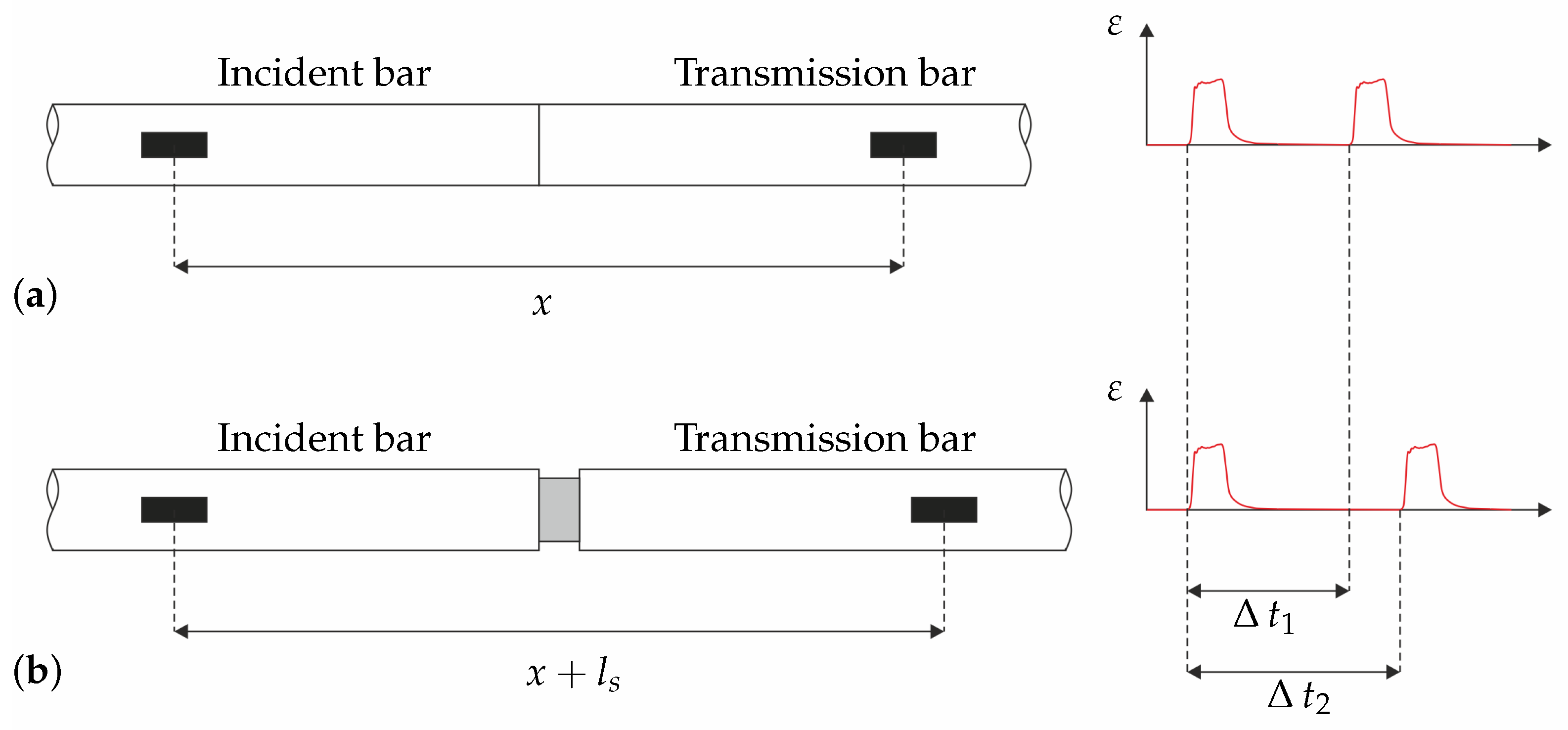
2.3. Wave Propagation Velocity

If the values of elastic modulus E and the density of the material $\rho$ are known, the wave propagation velocity can be calculated by $c=\sqrt{E/\rho }$. Since for very soft materials, E is often not specified by the manufacturer and it is also challenging to measure it, the wave propagation velocity in our specimens is determined using the SHPB setup. A sample of a defined length is clamped between the bars. With the sample, the wave induced by the striker requires more time to propagate from the strain gauge of the incident bar to the strain gauge of the transmission bar; see Figure 3. The recorded values can now be used to calculate the longitudinal wave propagation velocity of the sample’s material,

$$\begin{array}{c}\hfill c_{\mathrm{s}}={\displaystyle \frac{l_s}{\Delta t_{\mathrm{s}}}}\mathrm{where}\Delta t_{\mathrm{s}}=\Delta t_2-\Delta t_1\end{array}$$

(1)

where $l_s$ and $t_s$ are the length of the specimen and the additional time required for the wave to pass through the specimen. The values $\Delta t_1$ and $\Delta t_2$ show the time intervals between the signals measured by strain gauges at the incident and transmission bar with and without a specimen clamped between the bars. The method gives for Elastic a wave propagation velocity of $c_{\mathrm{s}}=98$ m/s. We remark that the procedure was calibrated with several measurements on the PMMA bars without specimens. Since the propagation velocity is constant, the shape of the measured signals is not important at this point.

2.4. Mechanical Impedance

The impedance indicates how fast a wave travels in the medium. For bars with constant diameter, it can be specified in a form that depends only on the material properties,

$$\begin{array}{cc}\hfill Z_0& =\sqrt{E\rho }=\rho c.\hfill \end{array}$$

(2)

Clearly, a stiff and dense material has a high impedance; e.g., for steel, we obtain $44\mathrm{kg}/{\mathrm{m}}^2\mathsf{\mu }$s; see

Table 2. Properties of bars made of different materials.

	Steel Bars	Aluminum Bars	PMMA Bars
length l	1800 mm	1800 mm	3000 mm/2200 mm
diameter d	20 mm	20 mm	20 mm
density $\rho$	7850 kg/m3	2700 kg/m3	1178 kg/m3
elastic modulus E	210 GPa	70 GPa	3.5 GPa
poisson number $\nu$	0.30	0.34	0.37
wave speed c	5645.2 m/s	5071.5 m/s	2295.9 m/s
impedance $Z_0$	44.31 kg/m2 $\mathsf{\mu }$s	13.69 kg/m2 $\mathsf{\mu }$s	2.58 kg/m2 $\mathsf{\mu }$s

. On the contrary, our silicon-like material has an impedance of $0.12\mathrm{kg}/{\mathrm{m}}^2\mathsf{\mu }$s. This mismatch mimics almost a free end of the bar and would lead to a full reflection of the compressive wave. No pulse could be measured at the strain gauge applied to the transmission bar.

Since the cross-section areas are also relevant when a longitudinal wave passes, the impedance needs to be calculated in the following form [30]:

$$\begin{array}{cc}\hfill Z& =A\sqrt{E\rho }=A\rho c\hfill \end{array}$$

(3)

From Equation (3), it follows that the impedance mismatch can be influenced by adjusting the material pairing and by varying the cross-sectional areas. There are several ways to deal with this situation. For example, the authors of [31,32] use a hollow transmission bar to reduce the specimen’s cross-section and thus the impedance mismatch. Another possibility is to increase the sensitivity of the strain gauges, especially on the transmission bar, cf. [33]. The simplest approach, which we also use here, is to substitute the metal bars with a plastic material that has naturally a much lower impedance.

However, with our choice of PMMA bars, other problems arise because of the material’s viscoelastic behavior. For the low attenuation and dispersion in metal bars, the signal measured at the strain gauges in the center of the bars represents nearly exactly the wave at every point of the bar. Unfortunately, this situation changes for the PMMA bar [34]. Due to the viscoelastic damping, it cannot be assumed that the pulse measured in the mid of the bar corresponds to the pulse at the bar’s end. Therefore the measured signal has to be corrected.

2.5. Reflection and Transmission Coefficients

In the following, ${\sigma }_{\mathrm{i}}$, ${\sigma }_{\mathrm{r}}$ and ${\sigma }_{\mathrm{t}}$ are the incident, reflected and transmitted stresses. In Figure 4, the situation is magnified for purposes of illustration. The equilibrium of forces at the surface of the incident bar $A_1$ and the specimen $A_2$ provides the relation,

$$\begin{array}{c}\hfill A_1\left({\sigma }_{\mathrm{i}}+{\sigma }_r\right)=A_2{\sigma }_{\mathrm{t}}\end{array}$$

(4)

and by solving it for ${\sigma }_{\mathrm{t}}$ and ${\sigma }_r$, we obtain the following expressions:

$$\begin{array}{c}\hfill {\sigma }_{\mathrm{t}}={\displaystyle \frac{A_1}{A_2}}\left({\sigma }_{\mathrm{i}}+{\sigma }_{\mathrm{r}}\right),{\sigma }_r={\displaystyle \frac{A_2}{A_1}}{\sigma }_{\mathrm{t}}-{\sigma }_{\mathrm{i}}\end{array}$$

(5)

The particle velocity v in a material is determined by the stress wave $\sigma \left(t\right)$, the material density $\rho$ and the wave speed c,

$$\begin{array}{c}\hfill v={\displaystyle \frac{\sigma }{\rho c}}.\end{array}$$

(6)

At the incident bar–specimen interface, the velocity is assumed to be continuous. Thus, at the impacted surface of the specimen, the following holds:

$$\begin{array}{c}\hfill {\displaystyle \frac{{\sigma }_{\mathrm{i}}-{\sigma }_{\mathrm{r}}}{{\rho }_1{c}_1}}={\displaystyle \frac{{\sigma }_{\mathrm{t}}}{{\rho }_2{c}_2}}\end{array}$$

(7)

With ${\sigma }_t$ of Equation (5) and ${\sigma }_i$ of Equation (7), we can calculate the reflection coefficient $\alpha$:

$$\begin{array}{c}\hfill \alpha ={\displaystyle \frac{{\sigma }_r}{{\sigma }_i}}={\displaystyle \frac{{\rho }_2{c}_2{A}_2-{\rho }_1{c}_1{A}_1}{{\rho }_1{c}_1{A}_1+{\rho }_2{c}_2{A}_2}}\end{array}$$

(8)

Accordingly, we can calculate the transmission coefficient $\beta$:

$$\begin{array}{c}\hfill \beta ={\displaystyle \frac{{\sigma }_{\mathrm{t}}}{{\sigma }_{\mathrm{i}}}}={\displaystyle \frac{{\rho }_2{c}_{2}2A_1}{{\rho }_1{c}_1{A}_1+{\rho }_2{c}_2{A}_2}}\end{array}$$

(9)

If we now substitute the impedance Z from Equation (3) into Equations (8) and (9), we obtain the equations in a more clearly arranged and more comfortable form:

$$\begin{array}{c}\hfill \alpha ={\displaystyle \frac{Z_2-Z_1}{Z_1+Z_2}},\beta ={\displaystyle \frac{2Z_2}{Z_1+Z_2}}.{\displaystyle \frac{A_1}{A_2}}\end{array}$$

(10)

The relations of Equation (10) show that for $Z_2\gg Z_1$, the reflection coefficient $\alpha$ is almost close to 1. That means nearly the entire wave is reflected at the interface, and no or only a very small portion of the wave is transmitted. As a consequence, no or only a weak pulse can be measured at the transmission bar.

Table 3. Impedance mismatch for material pairing of same cross-sectional areas.

Pairing	Reflection Coefficient $\mathit{\alpha }$	Transmission Coefficient $\mathit{\beta }$
Steel–EL	0.9945	6.6 × 10−3
Aluminum–EL	0.9826	0.0174
PMMA–EL	0.91	0.09

shows $\alpha$ and $\beta$ for different bar setups for the specimen under investigation.

2.6. Requirements for the SHPB Experiment

Summarizing, we state that for the evaluation of the SHPB experiments, three essential assumptions are typically made:

• A one-dimensional wave propagation in the bars;
• A state of equilibrium of forces in the compressed specimen, the “stress equilibrium”;
• A constant strain rate $\dot{\epsilon }$ during compression of the specimen.

The condition of one-dimensional wave propagation is fulfilled due to the experimental setup. Since the length-to-cross-sectional area ratio of the bars is about 1000, the 1D-wave equation applies:

$$\begin{array}{c}\hfill {c_b}^2{\displaystyle \frac{{\partial }^{2}u}{\partial x^2}}={\displaystyle \frac{{\partial }^{2}u}{\partial t^2}}\end{array}$$

(11)

Here, $u=u(x,t)$ is the displacement, and $c_b$ is the wave speed of the bar material.

To achieve a dynamic stress equilibrium, the stress, respectively, the force at both surfaces of the specimen has to be equal. However, it is challenging to meet this condition. In our experiments, the stress equilibrium condition $R\left(t\right)$ suggested by [35] is used. Stress equilibrium in the specimen is achieved when $R\left(t\right)$ approaches zero. Here, we have chosen $R\left(t\right)$ of less than 10% as an acceptable threshold value.

$$\begin{array}{c}\hfill R\left(t\right)=\left|{\displaystyle \frac{\Delta F\left(t\right)}{F_m}}\right|=2\left|{\displaystyle \frac{F_1-F_2}{F_1+F_2}}\right|\le 0.1\end{array}$$

(12)

In Equation (12) $F_1$, represents the force at the front side of the specimen, which is in contact with the incident bar, and $F_2$ indicates the force at the back end of the specimen. For this reason, the stress has to be known at two positions: at the end of the incident bar and the beginning of the transmission bar. However, strain gauges cannot be attached close to the interface because then the incident and the reflected pulses could no longer be distinguished. So, the strain gauge needs to be sufficiently far from the incident bar/specimen interface. As described above, the consequence is that the signal has to be corrected accordingly.

2.7. SHPB Equations

If all three requirements are met, the strain, strain rate, and stress in the specimen can be calculated as follows, cf. [36,37,38,39]; the indices b and s denote the bars and the specimen, respectively.

$$\begin{array}{cc}\hfill \dot{{\epsilon }_s}& =-2{\displaystyle \frac{c_b}{l_s}}{\epsilon }_r\hfill \end{array}$$

(13)

$$\begin{array}{cc}\hfill {\epsilon }_s& =-2{\displaystyle \frac{c_b}{l_s}}{\int }_{t_0}^t{\epsilon }_{r}dt\hfill \end{array}$$

(14)

$$\begin{array}{cc}\hfill {\sigma }_s& ={\displaystyle \frac{E_b{A}_b}{A_s}}{\epsilon }_t\hfill \end{array}$$

(15)

3. Signal Correction

For the evaluation of the SHPB experiment and Equations (13)–(15), the strains ${\epsilon }_r\left(t\right)$ and ${\epsilon }_r\left(t\right)$ at the interfaces of the incident bar–specimen and transmission bar–specimen are needed. However, they can only be measured at some distance from these interfaces. The strain gauges are typically applied at the middle of the long bars mainly to avoid interference between the incident and the reflected pulse.

Since polymeric bars like PMMA show some viscoelastic behavior, the interior attenuation and dispersion of the recorded signals are not negligible; see Figure 5. The signals recorded in the middle of the long bars do not correspond to the signal at the specimen’s interfaces.

Accordingly, the SHPB evaluation must be modified to determine the correct signal at the interfaces to the specimen. In the following, we outline a method to reconstruct the strain wave signal at the specimen from the signal recorded at locations far away from it.

For this reason, the measured data must be corrected accordingly. It has to be determined how the bar material’s damping properties affect the signal over certain distances.

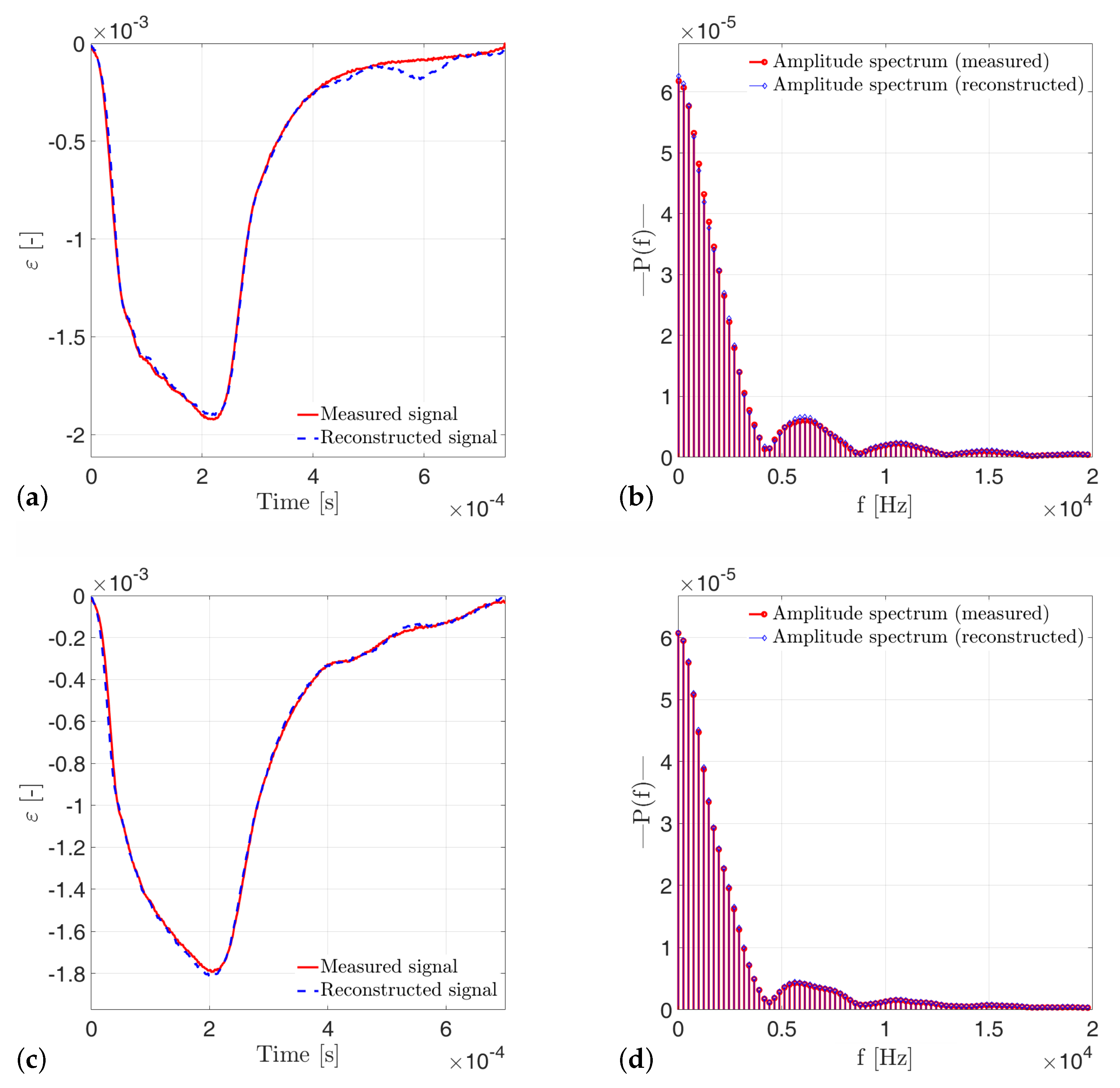
3.1. Correction by Spectral Analysis

Wave dispersion and attenuation in a long bar will be corrected by using digital signal processing methods. Fast Fourier Transform (FFT)-based spectral analysis algorithms are preferred for reconstructing the signal’s shape at the specific position, cf. [40,41]. To employ this correction method, it is necessary to measure the signal at more than one position. Therefore, for our experiments, the incident bar as well as the transmission bar are equipped with three strain gauges; see Figure 6.

Let us consider two strain gauges on the bar at positions $x_1$ and $x_2$. For the analysis, two signals $u_1$ and $u_2$ are measured at these positions. By using the FFT, the corresponding spectra are calculated, cf. [42]:

$$\begin{array}{cc}\hfill U_1\left(\omega \right)& =\mathrm{FFT}\left[u_1\left(t\right)\right]=\sum _n{U}_{1n}{e}^{i{\varphi }_{1n}}\hfill \end{array}$$

(16)

$$\begin{array}{cc}\hfill U_2\left(\omega \right)& =\mathrm{FFT}\left[u_2\left(t\right)\right]=\sum _n{U}_{2n}{e}^{i{\varphi }_{2n}}\hfill \end{array}$$

(17)

Here, $U_{1n}$, $U_{2n}$ represent the amplitude spectrum, and ${\varphi }_{1n}$, ${\varphi }_{2n}$ represent the phase spectrum of the respective spectral components. The change of the one-dimensional wave during the propagation can be described by two parameters, the attenuation factor ${\widehat{\alpha }}_n$ and the wavenumber ${\widehat{k}}_n$, [41]. The attenuation factor ${\widehat{\alpha }}_n$ can be calculated from the amplitudes $U_{1n}$ and $U_{2n}$.

$$\begin{array}{c}\hfill {\widehat{\alpha }}_n={\displaystyle \frac{\ln U_{1n}-\ln U_{2n}}{x_2-x_1}}\end{array}$$

(18)

The wavenumber ${\widehat{k}}_n$ is related to the wave dispersion and can be obtained from the calculated phases ${\varphi }_{1n}$ and ${\varphi }_{2n}$.

$$\begin{array}{c}\hfill {\widehat{k}}_n={\displaystyle \frac{{\varphi }_{1n}-{\varphi }_{2n}}{x_2-x_1}}\end{array}$$

(19)

We take the two signals and perform a spectral analysis to predict the spectrum of the pulse at a specific position of the bar. For that, we need the distance between the strain gauges receiving the pulses $(x_2-x_1)$.

Now, we can predict the wave signal at any location of the bar with distance $\Delta x$ from the measured signal,

$$\begin{array}{c}\hfill \Delta x=x_{\mathrm{m}}-x_{\mathrm{p}}\end{array}$$

(20)

where $x_{\mathrm{m}}$ is the position of the first measured signal and $x_{\mathrm{p}}$ is the position of the predicted wave. By using the FFT algorithm,

$$\begin{array}{c}\hfill U_{\mathrm{p}}(x,\omega )=U_{mn}{e}^{i{\varphi }_{mn}}{e}^{(-{\widehat{\alpha }}_n+i{\widehat{k}}_n)\Delta x}\end{array}$$

(21)

we obtain the predicted spectrum $U_{\mathrm{p}}(x,\omega )$.

Finally, the Inverse Fast Fourier Transformation (IFFT) reconstructs the wave at the desired location on the bar.

$$\begin{array}{c}\hfill u_{\mathrm{p}}=\mathrm{IFFT}\left[U_{\mathrm{p}}(x,\omega )\right]\end{array}$$

(22)

3.2. Validation of the Method

For validation, the SHPB experiment is carried out without a specimen between the bars. The positions of the strain gauges attached to the bars are shown in Figure 6. Three signals are measured on each bar for validation of the spectral analysis method for the reconstruction/prediction of a wave signal. We perform an FFT for the incident pulse signal measured at the strain gauges mounted at positions $x_1=850$ mm and $x_2=1500$ mm. Figure 7 shows the pulses of all three measuring positions cut from the signal for both bars. The signals were shifted to time zero to make it easier to compare them.

Based on the information about the signals obtained via the FFT at position $x_1$ and $x_2$, Equations (16)–(22) can be used to predict the signal at any location. In our case, we compare the predicted signal with the measured one at location $x_3=2150$ mm. Figure 8a shows the reconstructed and measured wave signals, whereas Figure 8b compares their amplitude spectrum. The measurements and predictions show a good match between the two signals. The same procedure was carried out for the strain gauges on the transmission bar. Here, however, the signal at the position $x_4=750$ mm was reconstructed on the basis of the signals at position $x_5=1250$ mm and $x_6=1750$ mm. An earlier pulse is therefore calculated here based on two pulses that occur later. This is applied analogously to the reflected impulse on the incident bar.

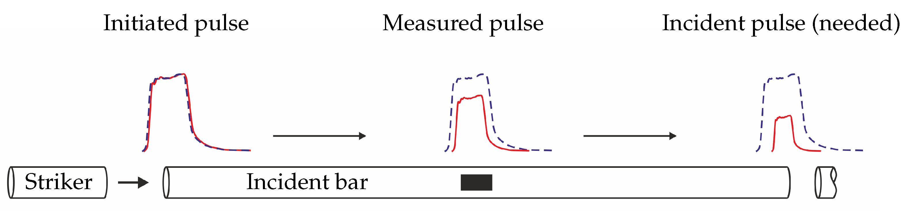
3.3. Signal Prediction

After successful validation of our signal correction method, we can now predict the strain wave at any position in the bar. Using Equations (16)–(22), the signal can be reconstructed at positions $x_{\mathrm{p}}$—in our case, at the interfaces of bars and specimen. The incident pulse is predicted based on previously measured signals, while the reflected and transmitted pulse are reconstructed based on later signals.

Figure 8. Comparison of measured predicted/corrected signals at position $x_3$: (a) incident pulse and (b) incident spectrum, (c) transmitted pulse and (d) transmitted spectrum.

Figure 8. Comparison of measured predicted/corrected signals at position $x_3$: (a) incident pulse and (b) incident spectrum, (c) transmitted pulse and (d) transmitted spectrum.

4. Experimental Results

We now perform the SHPB experiment with the Elastic material presented in Section 2.2 and

Table 4. Experimental setup.

	Bars	Striker	Specimen	Pulse Shaper
length [mm]	3000/2200	300	3	0.3
diameter [mm]	20	20	15	8
velocity [m/s]	-	11.5	-	-
material	PMMA	PMMA	Elastic	PE

. After prediction of the pulses, the signals can be analyzed according to Equations (13)–(15). The corrected pulses are plotted in Figure 9a. The striker speed for the experiments was chosen to 11 m/s. For the experimental setup, this results in a strain rate of approx. $\dot{\epsilon }$ = 2500 1/s. After a short time, a stress equilibrium $R\left(t\right)$ is achieved in the specimen, which fulfills the requirement of Equation (12); see Figure 9b.

A pulse shaper made of PE (polyethylene) with a diameter of 8 mm and a thickness of 0.3 mm was applied to the surface of the incident bar. The pulse shaper influences the waveform and eliminates high oscillations by elastic and plastic deformation during the impact [43]. It is needed here to achieve stress equilibrium, cf. [44,45].

The dynamic stress–strain curve has been determined from the measurements and is displayed in Figure 9a. From that stress–strain curve, the dynamic modulus of elasticity at the corresponding strain rate is deduced.

The modulus of elasticity of the silicone-like material is low and is rarely measured. In static tension tests, it reaches values up to 50 MPa [46]. Generally, in very soft materials, the modulus of elasticity increases significantly at high strain rates. That means we expect here a much higher modulus of elasticity.

The stress–strain curve in Figure 10 is plotted based on the corrected signals using Equations (13)–(15). Here, the modulus of elasticity is derived with the criteria of EN ISO 604 [47]. Therefore a linear regression is performed between ${\epsilon }_1^{*}$ = 0.0005 and ${\epsilon }_2^{*}$ = 0.0025, cf. Equation (23).

$$\begin{array}{c}\hfill E_{\mathrm{dyn}}={\displaystyle \frac{{\sigma }_{2\ast }-{\sigma }_{1\ast }}{{\epsilon }_{2\ast }-{\epsilon }_{1\ast }}}=297\mathrm{MPa}\end{array}$$

(23)

It should be noted that $E_{\mathrm{dyn}}$ depends on the strain rate. That means $E_{\mathrm{dyn}}$ is different for various strain rates, which is mainly due to a rate-dependent material response on the microscale.

5. Conclusions

This paper addresses the problems that arise for soft material testing in an SHPB setup. The silicone-like specimens were produced from liquid resin using a DLP process.

The very soft material has a low mechanical impedance. Thus, in the SHPB experiment, bars made of PMMA were used to reduce the impedance mismatch between bars and specimen material. The paper suggests a method to calculate wave signals at different locations of the SHPB bars and, thus, to correct the measured data.

The proposed procedure, based on a spectral analysis by FFT, provides a convenient technique for predicting and reconstructing pulses at various locations of the viscoelastic bars. For validation, the measured signals were compared to the predicted ones. The results of both signal shapes fit very well with each other.

After validation of the method, the SHPB experiment was performed with soft silicon-like specimens. Under static loading, the material has an elastic modulus of about $E=50$ MPa. The classical equations of the SHPB experiment are used to characterize the material under dynamic loading. From the measured stress–strain diagram, the elastic modulus was derived following the procedure of EN ISO 604. The results show a significant increase in the modulus of elasticity compared to the static case.

Since the stress–strain curve is only valid for the strain rate of our experiment, $\dot{\epsilon }=2500$, the measured dynamic elastic modulus of $E_{\mathrm{dyn}}=297$ MPa cannot be generalized. The experiment must be repeated for other strain rates with a setup adapted to the desired strain rate, e.g., by modifying the striker length and speed, the specimen geometry, or other parameters. Such experiments provide information about the material behavior at higher strain rates. Experiments with strain rates lower than 2500 1/s will show a lower elastic modulus than found in our investigation. However, it should still be above the static modulus of elasticity. For such experiments, the proposed signal correction method should be employed to calculate the actual strain at the specimen.

References

1. Perogamvros, N.; Mitropoulos, T.; Lampeas, G. Drop tower adaptation for medium strain rate tensile testing. Exp. Mech. 2006, 56, 419–436. [Google Scholar] [CrossRef]
2. Khosravani, M.; Weinberg, K. A review on split Hopkinson bar experiments on the dynamic characterisation of concrete. Constr. Build. Mater. 2018, 190, 1264–1283. [Google Scholar] [CrossRef]
3. Chen, W.; Song, B.; Frew, D.; Forrestal, M. Dynamic small strain measurements of a metal specimen with a split Hopkinson pressure bar. Exp. Mech. 2003, 43, 20–23. [Google Scholar] [CrossRef]
4. Kolsky, H. An Investigation of the Mechanical Properties of Materials at very High Rates of Loading. Proc. Phys. Soc. Sect. B 1949, 62, 676. [Google Scholar] [CrossRef]
5. Othman, R. The Kolsky-Hopkinson Bar Machine: Selected Topics; Springer Science & Business Media: New York, NY, USA, 2018. [Google Scholar]
6. Hopkinson, B.X. A method of measuring the pressure produced in the detonation of high, explosives or by the impact of bullets. Philos. Trans. R. Soc. Lond. Ser. A Contain. Pap. A Math. Phys. Character 1914, 213, 437–456. [Google Scholar]
7. Owens, A.; Tippur, H. A tensile split Hopkinson bar for testing particulate polymer composites under elevated rates of loading. Exp. Mech. 2009, 49, 799–811. [Google Scholar] [CrossRef]
8. Weinberg, K.; Khosravani, M.R. On the tensile resistance of UHPC at impact. Eur. Phys. J. Spec. Top. 2018, 227, 167–177. [Google Scholar] [CrossRef]
9. Zhao, J.; Knauss, W.; Ravichandran, G. Applicability of the time–temperature superposition principle in modeling dynamic response of a polyurea. Mech. Time-Depend. Mater. 2007, 11, 289–308. [Google Scholar] [CrossRef]
10. Deshpande, V.; Fleck, N. High strain rate compressive behaviour of aluminium alloy foams. Int. J. Impact Eng. 2000, 24, 277–298. [Google Scholar] [CrossRef]
11. Weinberg, K.; Khosravani, M.R.; Thimm, B.; Reppel, T.; Bogunia, L.; Aghayan, S.; Nötzel, R. Hopkinson bar experiments as a method to determine impact properties of brittle and ductile materials. GAMM-Mitteilungen 2018, 41, e201800008. [Google Scholar] [CrossRef]
12. Bieler, S.; Haller, S.; Brandt, R.; Weinberg, K. Experimental Investigation of Unidirectional Glass-Fiber-Reinforced Plastics under High Strain Rates. Appl. Mech. 2023, 4, 1127–1139. [Google Scholar] [CrossRef]
13. Green, S.; Schierloh, F.; Perkins, R.; Babcock, S. High-velocity deformation properties of polyurethane foams: Results of tensile and compressive tests at strain rates from 10−3 to 103 sec are presented for two kinds of polyurethane foam at various densities. Exp. Mech. 1969, 9, 103–109. [Google Scholar] [CrossRef]
14. Chawla, A.; Mukherjee, S.; Marathe, R.; Karthikeyan, B.; Malhotra, R. Determining strain rate dependence of human body soft tissues using a split Hopkinson pressure bar. In Proceedings of the International IRCOBI Conference on the Biomechanics of Impact, Madrid, Spain, 20–22 September 2006; pp. 20–22. [Google Scholar]
15. Trexler, M.; Lennon, A.; Wickwire, A.; Harrigan, T.; Luong, Q.; Graham, J.; Maisano, A.; Roberts, J.; Merkle, A. Verification and implementation of a modified split Hopkinson pressure bar technique for characterizing biological tissue and soft biosimulant materials under dynamic shear loading. J. Mech. Behav. Biomed. Mater. 2011, 4, 1920–1928. [Google Scholar] [CrossRef]
16. Chen, W.W.; Song, B. Dynamic Characterization of Soft Materials. Dyn. Fail. Mater. Struct. 2018, 19, 1–28. [Google Scholar]
17. Dwyer, C.M.; Carrillo, J.G.; De la Peña, J.A.D.; Santiago, C.C.; MacDonald, E.; Rhinehart, J.; Williams, R.M.; Burhop, M.; Yelamanchi, B.; Cortes, P. Impact performance of 3D printed spatially varying elastomeric lattices. Polymers 2023, 15, 1178. [Google Scholar] [CrossRef]
18. Kreide, C.; Koricho, E.; Kardel, K. Energy absorption of 3D printed multi-material elastic lattice structures. Prog. Addit. Manuf. 2024, 9, 1653–1665. [Google Scholar] [CrossRef]
19. Fíla, T.; Koudelka, P.; Falta, J.; Zlámal, P.; Rada, V.; Adorna, M.; Bronder, S.; Jiroušek, O. Dynamic impact testing of cellular solids and lattice structures: Application of two-sided direct impact Hopkinson bar. Int. J. Impact Eng. 2021, 148, 103767. [Google Scholar] [CrossRef]
20. Kang, S.G.; Gainov, R.; Heußen, D.; Bieler, S.; Sun, Z.; Weinberg, K.; Dehm, G.; Ramachandramoorthy, R. Green laser powder bed fusion based fabrication and rate-dependent mechanical properties of copper lattices. Mater. Des. 2023, 231, 112023. [Google Scholar] [CrossRef]
21. Bieler, S.; Kang, S.G.; Heußen, D.; Ramachandramoorthy, R.; Dehm, G.; Weinberg, K. Investigation of copper lattice structures using a Split Hopkinson Pressure Bar. PAMM 2021, 21, e202100155. [Google Scholar] [CrossRef]
22. Bieler, S.; Weinberg, K. Energy absorption of sustainable lattice structures under impact loading. arXiv 2024, arXiv:2412.06547. [Google Scholar]
23. Iftekar, S.F.; Aabid, A.; Amir, A.; Baig, M. Advancements and limitations in 3D printing materials and technologies: A critical review. Polymers 2023, 15, 2519. [Google Scholar] [CrossRef] [PubMed]
24. Gorham, D. Specimen inertia in high strain-rate compression. J. Phys. D Appl. Phys. 1989, 22, 1888. [Google Scholar] [CrossRef]
25. Gray III, G.; Blumenthal, W.R.; Trujillo, C.P.; Carpenter II, R. Influence of temperature and strain rate on the mechanical behavior of Adiprene L-100. J. Phys. IV 1997, 7, C3–C523. [Google Scholar]
26. Liu, Y.; Wang, Y.; Deng, Q. Radial Inertia Effect of Ultra-Soft Materials from Hopkinson Bar and Solution Methodologies. Materials 2024, 17, 3793. [Google Scholar] [CrossRef] [PubMed]
27. Chen, W.W.; Song, B. Split Hopkinson (Kolsky) Bar: Design, Testing and Applications; Springer Science & Business Media: New York, NY, USA, 2010. [Google Scholar]
28. Aghayan, S.; Bieler, S.; Weinberg, K. Determination of the high-strain rate elastic modulus of printing resins using two different split Hopkinson pressure bars. Mech. Time-Depend. Mater. 2022, 26, 761–773. [Google Scholar] [CrossRef]
29. Formlabs: Material Properties of Elastic Resin. 2025. Available online: https://formlabs.com/materials/flexible-elastic/ (accessed on 20 January 2025).
30. Graff, K.F. Wave Motion in Elastic Solids; Courier Corporation: Washington, DC, USA, 2012. [Google Scholar]
31. Chen, W.; Zhang, B.; Forrestal, M. A split Hopkinson bar technique for low-impedance materials. Exp. Mech. 1999, 39, 81–85. [Google Scholar] [CrossRef]
32. Chen, W.; Lu, F.; Frew, D.; Forrestal, M. Dynamic compression testing of soft materials. J. Appl. Mech. 2002, 69, 214–223. [Google Scholar] [CrossRef]
33. Chen, W.; Lu, F.; Zhou, B. A quartz-crystal-embedded split Hopkinson pressure bar for soft materials. Exp. Mech. 2000, 40, 1–6. [Google Scholar] [CrossRef]
34. Szabo, T.L.; Wu, J. A model for longitudinal and shear wave propagation in viscoelastic media. J. Acoust. Soc. Am. 2000, 107, 2437–2446. [Google Scholar] [CrossRef] [PubMed]
35. Ravichandran, G.; Subhash, G. Critical Appraisal of Limiting Strain Rates for Compression Testing of Ceramics in a Split Hopkinson Pressure Bar. J. Am. Ceram. Soc. 1994, 77, 263–267. [Google Scholar] [CrossRef]
36. Frew, D.; Forrestal, M.J.; Chen, W. Pulse shaping techniques for testing brittle materials with a split Hopkinson pressure bar. Exp. Mech. 2002, 42, 93–106. [Google Scholar] [CrossRef]
37. Van Sligtenhorst, C.; Cronin, D.S.; Brodland, G.W. High strain rate compressive properties of bovine muscle tissue determined using a split Hopkinson bar apparatus. J. Biomech. 2006, 39, 1852–1858. [Google Scholar] [CrossRef] [PubMed]
38. Sasso, M.; Newaz, G.; Amodio, D. Material characterization at high strain rate by Hopkinson bar tests and finite element optimization. Mater. Sci. Eng. A 2008, 487, 289–300. [Google Scholar] [CrossRef]
39. Song, Z.; Wang, Z.; Kim, H.; Ma, H. Pulse shaper and dynamic compressive property investigation on ice using a large-sized modified split hopkinson pressure bar. Lat. Am. J. Solids Struct. 2016, 13, 391–406. [Google Scholar] [CrossRef]
40. Bacon, C. An experimental method for considering dispersion and attenuation in a viscoelastic Hopkinson bar. Exp. Mech. 1998, 38, 242–249. [Google Scholar] [CrossRef]
41. Cheng, Z.; Crandall, J.; Pilkey, W. Wave dispersion and attenuation in viscoelastic split Hopkinson pressure bar. Shock Vib. 1998, 5, 307–315. [Google Scholar] [CrossRef]
42. Doyle, J.F. Wave Propagation in Structures: An FFT-Based Spectral Analysis Methodology; Springer Science & Business Media: Berlin/Heidelberg, Germany, 1989. [Google Scholar]
43. Gong, J.; Malvern, L.; Jenkins, D. Dispersion investigation in the split Hopkinson pressure bar. Int. J. Solids Struct. 1990, 112, 309–314. [Google Scholar] [CrossRef]
44. Vecchio, K.S.; Jiang, F. Improved pulse shaping to achieve constant strain rate and stress equilibrium in split-Hopkinson pressure bar testing. Metall. Mater. Trans. A 2007, 38, 2655–2665. [Google Scholar] [CrossRef]
45. Frew, D.; Forrestal, M.; Chen, W. Pulse shaping techniques for testing elastic-plastic materials with a split Hopkinson pressure bar. Exp. Mech. 2005, 45, 186–195. [Google Scholar] [CrossRef]
46. Sagar, S.K.; Sreekumar, M. Miniaturized flexible flow pump using SMA actuator. Procedia Eng. 2013, 64, 896–906. [Google Scholar] [CrossRef]
47. EN ISO 604. 2002. Available online: https://www.din.de/de/meta/suche/62730!search?query=druckeigenschaften (accessed on 20 January 2025).
Figure 1. Structure of the SHPB setup.
Dynamics 05 00005 g001
Figure 2. Steps of the sample manufacturing process.
Dynamics 05 00005 g002
Figure 3. Wave propagation velocity: (a) measurement without specimen and (b) with specimen between the bars.
Dynamics 05 00005 g003
Figure 4. Reflection and transmission of the pulse at the boundary surfaces.
Dynamics 05 00005 g004
Figure 5. Illustration of the typical wave attenuation and dispersion in polymeric bars (solid line) and metal bars (dashed line).
Dynamics 05 00005 g005
Figure 6. Location of the strain gauges with their corresponding signal placed on the incident bar (solid line) and transmission bar (dashed line).
Dynamics 05 00005 g006
Figure 7. Measured signals of the three strain gauges applicated to the incident bar (a) and to the transmission bar (b).
Dynamics 05 00005 g007
Figure 9. Corrected pulses of the measurement shifted to time zero (a) and the stress equilibrium of the corrected pulses (b).
Dynamics 05 00005 g009
Figure 10. Stress–strain curve for Elastic at ε ˙ = 2500 1/s.
Dynamics 05 00005 g010