Derivation of an Analytical Solution of a Forced Cantilevered Tube Conveying Fluid

Abstract

In this paper, an analytical technique is proposed to obtain the forced response of a cantilevered tube conveying fluid. By considering the pipe subjected to an arbitrary harmonic force, either distributed or concentrated, an analytical solution is found using Green’s function method. The closed-form solution obtained satisfies the differential equations governing the vibrating tube conveying fluid. The proposed method, which provides exact solutions, is more accurate than the classical eigenfunction expansion or Galerkin’s method and eliminates the need for eigenfunctions, eigenvalues, or infinite series.

1. Introduction

Pipes or tubes carrying fluid play a critical role in a wide range of engineering applications, including fuel pipelines, inkjet print-head nozzles, fuel-carrying tubes in space shuttle engines, heat exchangers, and piping systems in nuclear power plants. Understanding and controlling the forced vibrations of these tubes are essential for their efficient and safe operation [1,2]. Additionally, feedback control methods used for beam vibrations can be adapted to mitigate unwanted vibrations in fluid-conveying tubes [3].

From a theoretical standpoint, fluid–structure interactions involving moving boundary conditions remains one of the most challenging problems in dynamical systems. The term “moving boundary condition” refers to situations where the boundary—such as the walls of a tube—is not stationary but moves or deforms in response to external forces acting on the fluid-conveying tube. This dynamic boundary significantly complicates the analysis of fluid–structure interactions.

For over 50 years these complexities have been the focus of extensive theoretical and experimental research. The challenges that have been explored include changes in the natural frequencies of the pipe system due to flowing fluid, vibrations induced by turbulent flows, and instabilities such as flutter (via a Hopf bifurcation) that occur when the flow velocity reaches a critical threshold [4]. According to Weaver and Unny [5], the study of forced vibrations in pipes conveying fluid encompasses two main aspects: the physical aspect, which provides insights into the system’s dynamics, and the analytical aspect, which involves developing techniques to predict the forced response of such systems. This work focuses on developing analytical techniques to predict the forced responses of pipes conveying fluid, contributing to a better understanding of these complex systems. Understanding their stability and vibrational characteristics is essential for safety and performance in practical applications. For instance, Zhang and Li [6] investigated the dynamic stability of cantilevered pipes under various lateral distributed loads using the differential quadrature method, finding that descending distributed loads significantly enhance system stability. Sepehri-Amin et al. [7] examined the vibration of functionally graded damped beams with multiple fractionally damped absorbers, providing analytical and numerical solutions. Yang et al. [8] presented analytical solutions to peridynamic beam equations under static and dynamic loading, employing the central difference scheme for numerical solutions. Hozhabrossadati et al. [9] applied Green’s function method to uniform Euler–Bernoulli beams at resonant conditions, introducing the Fredholm Alternative Theorem, but without considering fluid interactions or pointwise forces. Advancements in analytical solutions for pipe flow include García-García and Alvariño [10,11], who developed analytical solutions for unsteady and transient turbulent pipe flow. As a simplified test case, they developed an analytical solution for starting turbulent pipe flow originated by a sudden pressure gradient increase, investigating the influence of Reynolds shear stress on velocity patterns in turbulent starting flows. Urbanowicz et al. [12,13] reviewed Navier–Stokes solutions for accelerating pipe flow and advanced wall shear-stress modeling for water hammer phenomena. Henclik [14] analyzed an analytical solution for water hammer in pipelines with elastically attached valves. Bayle and Plouraboué [15] proposed Laplace-domain fluid–structure interaction solutions for water hammer waves in a pipe. However, their approaches do not fully address the challenges associated with vibrating point forces in pipes conveying fluid.

This paper presents an improved analytical strategy based on the Green’s function method to develop closed-form solutions for a cantilevered tube conveying fluid, ensuring smoothness with continuous derivatives and satisfying the linear governing equations. The proposed method is applied under steady-flow conditions where the fluid velocity U, with a constant volumetric flow rate, is assumed to be constant. Additionally, the method does not require solving the free vibration problem to obtain eigenvalues and related eigenfunctions, which are typically necessary when using the classical Galerkin method.

2. Tube Conveying Fluid General Equation of Motion

The system under consideration is a straight cantilever tube fixed at one end on the x-axis. The fluid with an average velocity U enters the tube at the fixed end and exits at the free end. A force is applied to the tube, allowing it to move transversely, as depicted in Figure 1. Furthermore, the force that induces tube motion is assumed to be harmonic. Unlike the unconstrained pipe dynamical stability studied by many others [5,16], the goal here is considerably different in the sense that we want to know the precise deflection of the tube, with the harmonic force considered either distributed or concentrated.

Neglecting the effects of dissipation and damping, the general equation of motion for a tube conveying fluid can be formulated based on the following assumptions: (i) the tube has a uniform annular cross-section; (ii) the length of the tube is significantly greater than its diameter; (iii) the effects of rotary inertia and shear deformation are neglected; (iv) the tube’s centerline is inextensible; (v) the tube is elastic and initially straight; and (vi) cross-sections of the tube remain plane and perpendicular to the axis of the pipe containing a flowing liquid, in accordance with the Bernoulli–Euler beam theory. The equation governing the transverse displacement $v(x,t)$ can be expressed as follows [1,17]:

$$EI{\displaystyle \frac{{\partial }^{4}v}{\partial x^4}}+M_f{U}^2{\displaystyle \frac{{\partial }^{2}v}{\partial x^2}}+2U{M}_f{\displaystyle \frac{{\partial }^{2}v}{\partial t\partial x}}+(m_t+M_f){\displaystyle \frac{{\partial }^{2}v}{\partial t^2}}=F(x,t)$$

(1)

where $EI$ is the flexural rigidity of the beam, $M_f$ is the mass per unit length of the fluid, $m_t$ is the mass per unit length of the beam, and $F(x,t)$ is the applied force as a function of position and time.

3. Exact Analytical Solution

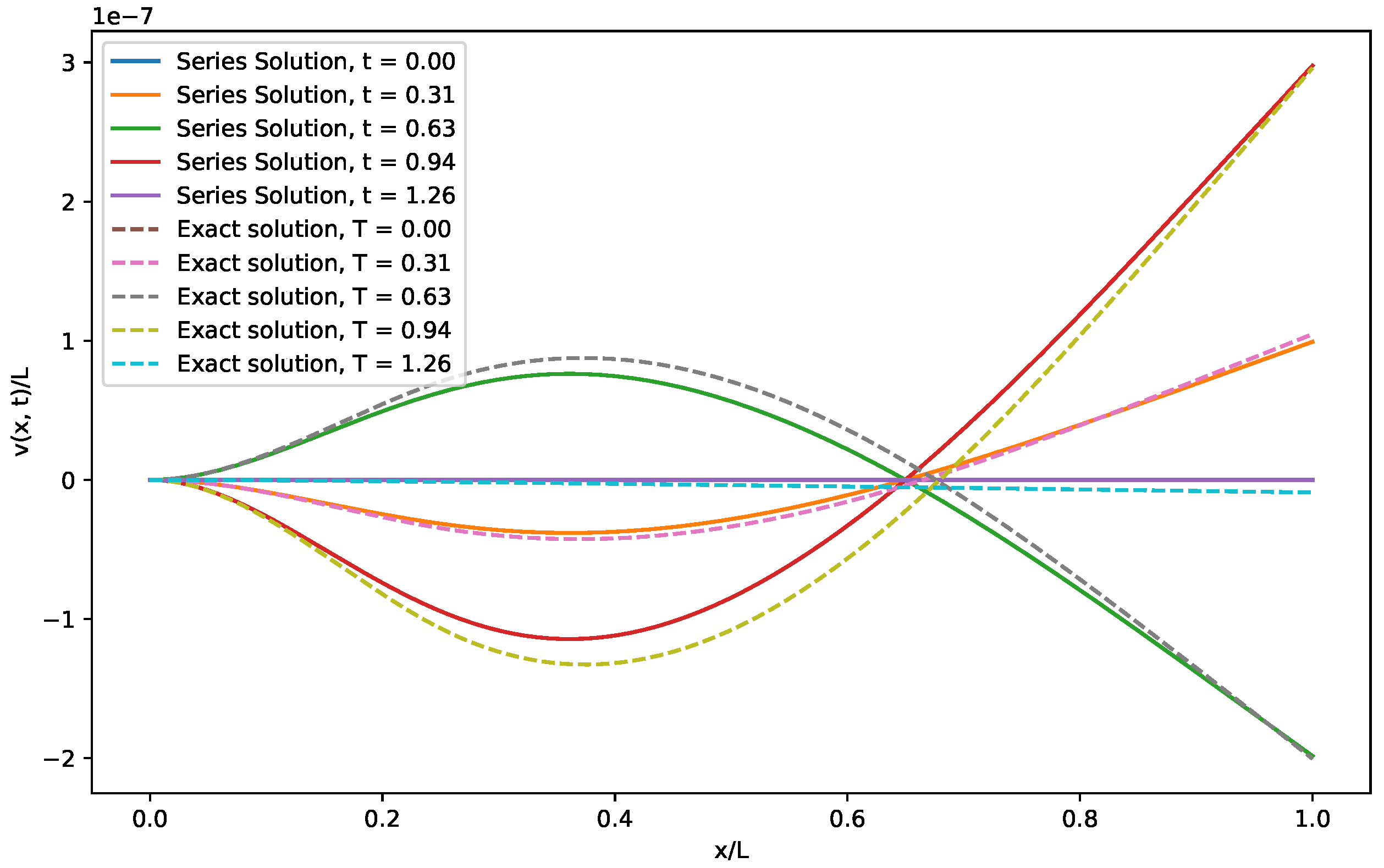
We propose an approach based on Green’s function method to solve Equation (1). Assuming the applied force is harmonic and localized, it can be represented as a point force:

$$F(x,t)=F_p\delta (x-x_p)sin\left({\Omega }_{p}t\right),$$

(2)

where $F_p$ is the amplitude of the force, ${\Omega }_p$ is the frequency, and $\delta (x-x_p)$ represents a Dirac delta function centered at $x_p$, indicating that the force is applied at position $x_p$. For convenience, we reformulate the problem in a complex form by expressing the sinusoidal force as

$$F(x,t):=F_p\delta (x-x_p)e^{j({\Omega }_{p}t-\pi /2)},$$

(3)

where $e^{i{\Omega }_{p}t}$ is the complex representation of the time-dependent oscillation. This allows us to work with simpler exponential functions, therefore simplifying the analysis of the system’s harmonic response using Green’s function.

Green’s function technique is a well-known method for solving PDEs. A Green’s function is the solution of the equation subject to a unit impulse. The technique can be applied as detailed below. We consider the general governing equation

$$\mathcal{L}u\left(\overrightarrow{x}\right)=h\left(\overrightarrow{x}\right),$$

(4)

where $\mathcal{L}$ is a linear differential operator that involves derivatives with respect to spatial variables and possibly time. It acts on the unknown function $u\left(\overrightarrow{x}\right)$, which depends on the spatial coordinates $\overrightarrow{x}$–which could represent (x,y,z) in 3D. The term $h\left(\overrightarrow{x}\right)$ is a known function that represents the external forcing applied to the system. The objective is to determine $u\left(\overrightarrow{x}\right)$ such that this equation is satisfied for the given $h\left(\overrightarrow{x}\right)$.

We assume that the following equation, when solved with an impulse, yields Green’s function $G(\overrightarrow{x},\overrightarrow{x^{\prime }})$ as the solution:

$$\mathcal{L}G(\overrightarrow{x},\overrightarrow{x^{\prime }})=\delta (\overrightarrow{x}-\overrightarrow{x^{\prime }}),$$

(5)

where $\delta (\overrightarrow{x}-\overrightarrow{x^{\prime }})$ is the Dirac delta function. In addition, we can express

$$h\left(\overrightarrow{x}\right)=\int h\left({\overrightarrow{x}}^{\prime }\right)\delta (\overrightarrow{x}-{\overrightarrow{x}}^{\prime })d\overrightarrow{x^{\prime }};$$

(6)

using (5), and, with the linearity of (4), one obtains

$$u\left(\overrightarrow{x}\right)=\int G(\overrightarrow{x},\overrightarrow{x^{\prime }})h\left({\overrightarrow{x}}^{\prime }\right)d\overrightarrow{x^{\prime }}.$$

(7)

In the following, this result will be applied to solve the equation of motion of a forced tube conveying fluid with $\overrightarrow{x}$ simplified to x.

Based on the forcing term in (3), the solution of our problem is sought as

$$w(x,t)=V\left(x\right)e^{j({\Omega }_{p}t-\pi /2)},$$

(8)

where $V\left(x\right)$ is a function that describes the spatial variation of the solution. In addition, the solution $v(x,t)$ of (1) is the real part of $w(x,t)$. By substituting (8) into (1), we obtain

$$V^{\prime \prime \prime \prime }\left(x\right)+a{V}^{\prime \prime }\left(x\right)+jb{V}^{\prime }\left(x\right)-cV\left(x\right)={\displaystyle \frac{F_p\delta (x-x_p)}{EI}},$$

(9)

where $a=M_f{U}^2/EI$, $b=2M_{f}U{\Omega }_p/EI$ and $c=(m_t+M_f){\Omega }_p^2/EI$, the solution of which is given by

$$V\left(x\right)={{\displaystyle \frac{F_p}{EI}}}_0^L\delta (x^{\prime }-x_p)G(x,x^{\prime })d{x}^{\prime }={\displaystyle \frac{F_p}{EI}}G(x,x_p),$$

(10)

where we determine the Green’s function by solving the following equation:

$$V^{\prime \prime \prime \prime }\left(x\right)+a{V}^{\prime \prime }\left(x\right)+jb{V}^{\prime }\left(x\right)-cV\left(x\right)=\delta (x-x^{\prime }),$$

(11)

which is performed by adopting the Laplace transform and its inverse. We then deduce

$$\begin{array}{c}G(x,x^{\prime })=\mathrm{H}(x-x^{\prime }){\displaystyle \sum _{i=1}^4}{\displaystyle \frac{e^{{\alpha }_i(x-x^{\prime })}}{4{{\alpha }_i}^3+2{\alpha }_{i}a+jb}}\hfill \\ +V\left(0\right){\displaystyle \sum _{i=1}^4}{\displaystyle \frac{{{\alpha }_i}^3{e}^{{\alpha }_{i}x}}{4{{\alpha }_i}^3+2{\alpha }_{i}a+jb}}+V^{\prime }\left(0\right){\displaystyle \sum _{i=1}^4}{\displaystyle \frac{{{\alpha }_i}^2{e}^{{\alpha }_{i}x}}{4{{\alpha }_i}^3+2{\alpha }_{i}a+jb}}\hfill \\ +{\displaystyle \sum _{i=1}^4}{\displaystyle \frac{e^{{\alpha }_{i}x}}{4{{\alpha }_i}^3+2{\alpha }_{i}a+jb}}(V^{\prime \prime \prime }\left(0\right)+a{V}^{\prime }\left(0\right)+jbV\left(0\right))\hfill \\ +{\displaystyle \sum _{i=1}^4}{\displaystyle \frac{{\alpha }_i{e}^{{\alpha }_{i}x}}{4{{\alpha }_i}^3+2{\alpha }_{i}a+jb}}(V^{\prime \prime }\left(0\right)+aV\left(0\right)),\hfill \end{array}$$

(12)

where $H\left(x\right)$ is the Heaviside or step function,

$$\mathrm{H}\left(x\right):=\left\{\begin{array}{cc}0\hfill & \mathrm{if} x<0\hfill \\ 1\hfill & \mathrm{if} x\ge 0,\hfill \end{array}\right.$$

(13)

and ${\alpha }_i$, $1\le i\le 4$ are the solutions of the following polynomial equation:

$$Z^4+a{Z}^2+jbZ-c=0.$$

(14)

This equation can be analytically solved using Ferrari’s method [18].

Let $\psi \left(x\right)$ be the function defined as

$$\psi \left(x\right)=\sum _{i=1}^4{\displaystyle \frac{e^{{\alpha }_{i}x}}{4{\alpha }_i^3+2{\alpha }_{i}a+jb}}.$$

(15)

We then can write (12) in the following form:

$$\begin{array}{c}G(x,x^{\prime })=\mathrm{H}(x-x^{\prime })\psi (x-x^{\prime })+\left[{\psi }^{\prime \prime \prime }\left(x\right)+a{\psi }^{\prime }\left(x\right)+jb\psi \left(x\right)\right]V\left(0\right)\hfill \\ +[{\psi }^{\prime \prime }\left(x\right)+a\psi \left(x\right)]V^{\prime }\left(0\right)+{\psi }^{\prime }\left(x\right)V^{\prime \prime }\left(0\right)+\psi \left(x\right)V^{\prime \prime \prime }\left(0\right).\hfill \end{array}$$

(16)

The last step is now to decide on the different boundary conditions. For this purpose, we use the boundary conditions for the cantilever tube. At the fixed end ($x=0$), the deflection $v\left(x\right)$ is zero, i.e., $v\left(0\right)=0$, and the slope ${\displaystyle \frac{dv\left(x\right)}{dx}}=0$. At the free end ($x=L$), both the bending moment $EI{\displaystyle \frac{d^{2}v\left(x\right)}{d{x}^2}}$ and the shear force $EI{\displaystyle \frac{d^{3}v\left(x\right)}{d{x}^3}}$ are zero. Applying this to (16) leads to:

$$V^{\prime \prime }\left(L\right)=0={\psi }^{\prime \prime }(L-x^{\prime })+{\psi }^{\prime \prime \prime }\left(L\right)V^{\prime \prime }\left(0\right)+{\psi }^{\prime \prime }\left(L\right)V^{\prime \prime \prime }\left(0\right),$$

(17)

$$V^{\prime \prime \prime }\left(L\right)=0={\psi }^{\prime \prime \prime }(L-x^{\prime })+{\psi }^{\left(4\right)}\left(L\right)V^{\prime \prime }\left(0\right)+{\psi }^{\prime \prime \prime }\left(L\right)V^{\prime \prime \prime }\left(0\right),$$

(18)

where we use the fact that $0<x^{\prime }\le L$ along the tube, thus leading to $\mathrm{H}(L-x^{\prime })=1$ and $\mathrm{H}(0-x^{\prime })=0$.

Solving the previous Equations (17) and (18) leads to the determination of unknown boundary conditions:

$$V^{\prime \prime }\left(0\right)={\displaystyle \frac{{\psi }^{\prime \prime }\left(L\right){\psi }^{\prime \prime \prime }(L-x^{\prime })-{\psi }^{\prime \prime \prime }\left(L\right){\psi }^{\prime \prime }(L-x^{\prime })}{{\psi }^{\prime \prime \prime }{\left(L\right)}^2-{\psi }^{\prime \prime }\left(L\right){\psi }^{\left(4\right)}\left(L\right)}},$$

(19)

$$V^{\prime \prime \prime }\left(0\right)={\displaystyle \frac{{\psi }^{\left(4\right)}\left(L\right){\psi }^{\prime \prime }(L-x^{\prime })-{\psi }^{\prime \prime \prime }\left(L\right){\psi }^{\prime \prime \prime }(L-x^{\prime })}{{\psi }^{\prime \prime \prime }{\left(L\right)}^2-{\psi }^{\prime \prime }\left(L\right){\psi }^{\left(4\right)}\left(L\right)}}.$$

(20)

Finally, we can deduce the Green’s function of a tube conveying fluid as

$$\begin{array}{c}G(x,x^{\prime })=\mathrm{H}(x-x^{\prime })\psi (x-x^{\prime })\hfill \\ +{\displaystyle \frac{{\psi }^{\prime \prime }\left(L\right){\psi }^{\prime \prime \prime }(L-x^{\prime })-{\psi }^{\prime \prime \prime }\left(L\right){\psi }^{\prime \prime }(L-x^{\prime })}{{\psi }^{\prime \prime \prime }{\left(L\right)}^2-{\psi }^{\prime \prime }\left(L\right){\psi }^{\left(4\right)}\left(L\right)}}{\psi }^{\prime }\left(x\right)\hfill \\ +{\displaystyle \frac{{\psi }^{\left(4\right)}\left(L\right){\psi }^{\prime \prime }(L-x^{\prime })-{\psi }^{\prime \prime \prime }\left(L\right){\psi }^{\prime \prime \prime }(L-x^{\prime })}{{\psi }^{\prime \prime \prime }{\left(L\right)}^2-{\psi }^{\prime \prime }\left(L\right){\psi }^{\left(4\right)}\left(L\right)}}\psi \left(x\right).\hfill \end{array}$$

(21)

Using (10), we can finally establish the analytical solution of a tube conveying a fluid with a constant flow rate submitted to a punctual harmonic excitation as

$$v(x,t)=\Re \left[w\right(x,t\left)\right],$$

(22)

where $w(x,t)$ is given by

$$\begin{array}{c}w(x,t)={\displaystyle \frac{F_p}{EI}}exp\left[j({\Omega }_{p}t-\pi /2)\right]\{\mathrm{H}(x-x_p)\psi (x-x_p)\hfill \\ +{\displaystyle \frac{{\psi }^{\prime \prime }\left(L\right){\psi }^{\prime \prime \prime }(L-x_p)-{\psi }^{\prime \prime \prime }\left(L\right){\psi }^{\prime \prime }(L-x_p)}{{\psi }^{\prime \prime \prime }{\left(L\right)}^2-{\psi }^{\prime \prime }\left(L\right){\psi }^{\left(4\right)}\left(L\right)}}{\psi }^{\prime }\left(x\right)\hfill \\ +{\displaystyle \frac{{\psi }^{\left(4\right)}\left(L\right){\psi }^{\prime \prime }(L-x_p)-{\psi }^{\prime \prime \prime }\left(L\right){\psi }^{\prime \prime \prime }(L-x_p)}{{\psi }^{\prime \prime \prime }{\left(L\right)}^2-{\psi }^{\prime \prime }\left(L\right){\psi }^{\left(4\right)}\left(L\right)}}\psi \left(x\right)\}.\hfill \end{array}$$

(23)

4. Model Validation

We will validate the model by comparison with the series solutions, which are only valid for a tube without fluid, i.e., U = 0. It is worth noting that the cantilevered beam subjected to a pointwise force can be solved analytically, and the summary of the solution (see Appendix A) is provided below, with the point force being represented as

$$F(x,t)=F_p\delta (x-x_p)sin\left({\Omega }_{p}t\right).$$

(24)

Using separation of variables, the analytical solution can be written as (see Appendix A):

$$v(x,t)=\sum _{i=1}^N{\displaystyle \frac{F_p{V}_i\left(x_p\right)}{m_{t}L({\omega }_i^2-{\Omega }_p^2)}}{V}_i\left(x\right)sin\left({\Omega }_{p}t\right).$$

(25)

This represents the response of the empty tube (or cantilevered beam) in terms of its mode shapes (eigenfunctions) $(V_i\left(x\right)$ and natural frequencies ${\omega }_i$

$$V_i\left(x\right)=cosh\left({\beta }_{i}x\right)-cos\left({\beta }_{i}x\right)-\left({\displaystyle \frac{sinh\left({\beta }_{i}L\right)-sin\left({\beta }_{i}L\right)}{cosh\left({\beta }_{i}L\right)+cos\left({\beta }_{i}L\right)}}\right)(sinh\left({\beta }_{i}x\right)-sin\left({\beta }_{i}x\right)),$$

(26)

with

$${\omega }_i={\beta }_i^2\sqrt{{\displaystyle \frac{EI}{m_t}}}$$

(27)

obtained from the characteristic equation,

$$cos\left({\beta }_{i}L\right)cosh\left({\beta }_{i}L\right)+1=0.$$

(28)

The results of the comparison between the series and closed-form Green’s function solution are detailed below. The properties of the tube and fluid are shown in

Table 1. Tube and fluid properties used for the model validation.

Parameters	Value	Description	Unit
L	[1, 10, 15]	Length	m
${\rho }_t$	7800	Density of the material	kg/m3
${\rho }_f$	[0, 1000]	Fluid density	kg/m3
$r_{\mathrm{inner}}$	0.05	Tube inner radius	m
$r_{\mathrm{outer}}$	0.06	Tube outer radius	m
E	$2\times {10}^{11}$	Young’s modulus	Pa
U	[0, 0.1, 1]	Velocity	m/s
${\Omega }_p$	10.0	Excitation frequency	rad/s
$F_p$	10.0	Amplitude of the forcing function	N
$x_p$	L/4	Position where the force is applied	m
I	$I={\displaystyle \frac{\pi }{4}}(r_{\mathrm{outer}}^4-r_{\mathrm{inner}}^4)$	Area moment of inertia	-
$m_t$	$m_t={\rho }_t\pi (r_{\mathrm{outer}}^2-r_{\mathrm{inner}}^2)$	Mass per unit length of the tube	-
$M_f$	$M_f={\rho }_f\pi r_{\mathrm{inner}}^2$	Added mass per unit length due to fluid	-
a	$a={\displaystyle \frac{M_f{U}^2}{EI}}$	-
b	$b={\displaystyle \frac{M_{f}U{\Omega }_p}{EI}}$	-	-
c	$c={\displaystyle \frac{(m_t+M_f){\Omega }_p^2}{EI}}$	-	-

. As we can see in Figure 2 and Figure 3, a very good agreement is found for an empty tube, while the effect of the fluid can be observed in Figure 4 in terms of the tube’s transient deflection.

However, the fluid velocity does not affect the pipe deflection, as shown below when the length of the tube is taken as L = 1 m (Figure 5).

5. Conclusions

Considering a general equation of motion for a tube-carrying fluid subjected to harmonic excitation, an analytical technique based on the Green’s function method has been developed to find a solution for a tube conveying fluid. The derived exact solution is more accurate than the conventional series expansion or Galerkin’s method, and it does not require knowledge of the free vibration problem’s eigenfunctions or eigenvalues. The proposed method might also be extended to include moment solicitation and other configurations, such as multi-span tubes, different boundary conditions, and structural vibrations.

References

1. Paidoussis, M.P. Fluid-Structure Interactions: Slender Structures and Axial Flow, 2nd ed.; Academic Press: Amsterdam, The Netherlands; Boston, MA, USA, 2014. [Google Scholar]
2. Tembely, M.; Lecot, C.; Soucemarianadin, A. Prediction and evolution of drop-size distribution for a new ultrasonic atomizer. Appl. Therm. Eng. 2011, 31, 656–667. [Google Scholar] [CrossRef]
3. Lin, Y.H.; Chu, C.L. Active Flutter Control Of A Cantilever Tube Conveying Fluid Using Piezoelectric Actuators. J. Sound Vib. 1996, 196, 97–105. [Google Scholar] [CrossRef]
4. Housner, G.W. Bending Vibrations of a Pipe Line Containing Flowing Fluid. J. Appl. Mech. 2021, 19, 205–208. [Google Scholar] [CrossRef]
5. Weaver, D.S.; Unny, T.E. On the Dynamic Stability of Fluid-Conveying Pipes. J. Appl. Mech. 1973, 40, 48–52. [Google Scholar] [CrossRef]
6. Zhang, Y.; Li, P. Dynamical stability of pipe conveying fluid with various lateral distributed loads. Arch. Appl. Mech. 2023, 93, 4093–4106. [Google Scholar] [CrossRef]
7. Sepehri-Amin, S.; Faal, R.; Das, R. Analytical and numerical solutions for vibration of a functionally graded beam with multiple fractionally damped absorbers. Thin-Walled Struct. 2020, 157, 106711. [Google Scholar] [CrossRef]
8. Yang, Z.; Naumenko, K.; Altenbach, H.; Ma, C.C.; Oterkus, E.; Oterkus, S. Some analytical solutions to peridynamic beam equations. ZAMM—J. Appl. Math. Mech. Z. FüR Angew. Math. Und Mech. 2022, 102, e202200132. [Google Scholar] [CrossRef]
9. Hozhabrossadati, S.M.; Aftabi Sani, A.; Mehri, B.; Mofid, M. Green’s function for uniform Euler–Bernoulli beams at resonant condition: Introduction of Fredholm Alternative Theorem. Appl. Math. Model. 2015, 39, 3366–3379. [Google Scholar] [CrossRef]
10. García García, F.J.; Fariñas Alvariño, P. On an analytic solution for general unsteady/transient turbulent pipe flow and starting turbulent flow. Eur. J. Mech.—B/Fluids 2019, 74, 200–210. [Google Scholar] [CrossRef]
11. García García, F.J.; Fariñas Alvariño, P. On the influence of Reynolds shear stress upon the velocity patterns generated in turbulent starting pipe flow. Phys. Fluids 2020, 32, 105119. [Google Scholar] [CrossRef]
12. Urbanowicz, K.; Bergant, A.; Stosiak, M.; Deptuła, A.; Karpenko, M. Navier-Stokes solutions for accelerating pipe flow—A review of analytical models. Energies 2023, 16, 1407. [Google Scholar] [CrossRef]
13. Urbanowicz, K.; Bergant, A.; Stosiak, M.; Karpenko, M.; Bogdevičius, M. Developments in analytical wall shear stress modelling for water hammer phenomena. J. Sound Vib. 2023, 562, 117848. [Google Scholar] [CrossRef]
14. Henclik, S. Analytical solution and numerical study on water hammer in a pipeline closed with an elastically attached valve. J. Sound Vib. 2018, 417, 245–259. [Google Scholar] [CrossRef]
15. Bayle, A.; Plouraboué, F. Laplace-domain fluid–structure interaction solutions for water hammer waves in a pipe. J. Hydraul. Eng. 2023, 150, 04023062-1–12. [Google Scholar] [CrossRef]
16. Païdoussis, M.P.; Semler, C.; Wadham-Gagnon, M.; Saaid, S. Dynamics of cantilevered pipes conveying fluid. Part 2: Dynamics of the system with intermediate spring support. J. Fluids Struct. 2007, 23, 569–587. [Google Scholar] [CrossRef]
17. Ammari, K.; Tucsnak, M. Stabilization of Bernoulli–Euler Beams by Means of a Pointwise Feedback Force. SIAM J. Control Optim. 2000, 39, 1160–1181. [Google Scholar] [CrossRef]
18. Spiegel, M.R. Mathematical Handbook of Formulas and Tables, 1st ed.; Schaum, McGraw-Hill: New York, NY, USA, 1968. [Google Scholar]
Figure 1. Schematic of a tube along the x-axis conveying fluid with velocity U, subjected to an external force F ( x , t ) .
Dynamics 04 00046 g001
Figure 2. A comparison between the series and exact solution of a tube conveying fluid with L = 10 m, U = 0 m/s.
Dynamics 04 00046 g002
Figure 3. A comparison between the series and exact solution of an empty tube with L = 15 m, U = 0 m/s.
Dynamics 04 00046 g003
Figure 4. A comparison between the series and the exact solution of a tube conveying fluid with L = 15 m, U = 0.1 m/s.
Dynamics 04 00046 g004
Figure 5. A comparison between the series and exact solution of a tube conveying fluid with L = 1 m, U = 1 m/s.
Dynamics 04 00046 g005