Evaluation and Selection Models for Ensemble Intrusion Detection Systems in IoT

Abstract

Using the Internet of Things (IoT) for various applications, such as home and wearables devices, network applications, and even self-driven vehicles, detecting abnormal traffic is one of the problematic areas for researchers to protect network infrastructure from adversary activities. Several network systems suffer from drawbacks that allow intruders to use malicious traffic to obtain unauthorized access. Attacks such as Distributed Denial of Service attacks (DDoS), Denial of Service attacks (DoS), and Service Scans demand a unique automatic system capable of identifying traffic abnormality at the earliest stage to avoid system damage. Numerous automatic approaches can detect abnormal traffic. However, accuracy is not only the issue with current Intrusion Detection Systems (IDS), but the efficiency, flexibility, and scalability need to be enhanced to detect attack traffic from various IoT networks. Thus, this study concentrates on constructing an ensemble classifier using the proposed Integrated Evaluation Metrics (IEM) to determine the best performance of IDS models. The automated Ranking and Best Selection Method (RBSM) is performed using the proposed IEM to select the best model for the ensemble classifier to detect highly accurate attacks using machine learning and deep learning techniques. Three datasets of real IoT traffic were merged to extend the proposed approach’s ability to detect attack traffic from heterogeneous IoT networks. The results show that the performance of the proposed model achieved the highest accuracy of 99.45% and 97.81% for binary and multi-classification, respectively.

1. Introduction

Internet of Things (IoT) is a network that uses unique identifiers (UIDs) to connect things, including but not limited to computing devices, automatic and digital tools, objects, creatures, and people with the capacity to share data without needing human-to-human or human-to-computer interaction. IoT connects the physical and virtual worlds in simple terms. The fundamental idea behind IoT is to establish a safe, self-governing connection that allows data to be exchanged between real-world physical objects and apps [1]. The IoT Analytics report indicates that more than 11 billion IoT devices are connected and used in our current lives. Moreover, it is shown that there is an increase of more than 10% of IoT devices. The expectation is that in 2025, there will be around 21 billion IoT devices connected around the world [1]. As a result, the IoT has experienced rapid expansion in recent years due to widespread adoption in various sectors and industries, including smart cities and smart homes, agriculture, transportation, logistics, and healthcare [2]. The integration of IoT with growing and rapidly rising software such as Artificial Intelligence (AI), big data, and 5G is also receiving much attention. However, as the world becomes more interconnected through the Internet and the IoT ecosystem grows in size, application, connectivity, and complexity, the need to adequately secure IoT components at all levels, from physical to user, becomes more vital than ever. As a consequence, network security becomes essential. Advanced hacking techniques can compromise the security of IoT communications and computational components. There are numerous attacks in IoT networks, including but not limited to Denial of Service (DoS) and Distributed DoS (DDoS). This type of attacks can make the device unreachable to handle actual demands by flooding and over-burdening the IoT device with pointless and superfluous messages. The other type of attack is the Replay attack. This attack can be executed by capturing the traffic to distinguish the unencrypted information, which works with hackers to accomplish Man-in-the-Middle (MITM). Additionally, a spoofing attack where attackers can take on the appearance of legitimate clients and forward fake Global Positioning System (GPS) information to the nodes. Therefore, IDS is crucial to protect IoT from these attacks and secure the network by detecting abnormal behaviours using artificial intelligence [3]. IDS is usually divided into two types: anomaly and misuse methods that depend on being signature-based. Various types of machine and deep learning models for IDS have been published and trained to detect essential and specific threats for conventional networks and partly in the Internet of Things networks [4].

The heterogeneous IoT networks utilize various protocols and sub-connected systems, which makes learning different traffic patterns challenging for a single model. Integrating different learning models will increase the selection of the best model performance and decrease the risk of selecting a poorly performing classifier. Furthermore, integrating models with different decisions may yield a more reasonable result than any individual result. Therefore, an ensemble approach is required to enhance the model’s classification accuracy. However, an individual model’s performance sometimes overcomes such an approach, but it is guaranteed that the ensemble approach will decrease the total risk of invalid selection [4]. In general, hard and soft voting are the two main approaches to combining models decisions [5]. In hard voting, also known as majority voting, each classifier votes for a class, and the class with the most votes is chosen. More than half of the approaches make the same decision, which is referred to as the majority. Soft voting in the other hands, involves predicting the class based on a classifier’s anticipated probability (p) [6]. That is why soft voting is more reliable than hard voting since it examines more information and includes the weight of each classifier in the decision. Detecting cyberattacks on IoT networks requires IDS. However, the majority of IDSs can not successfully meet IoT networks’ requirements in the real world. The current IDS suffers from many false alarms and low detection accuracy. Moreover, the IoT network is extended rapidly by adding more connected devices every day, making designing a scalable and efficient IDS problematic. An ensemble detection approach is proposed in this study to accomplish a dependable, scalable, adaptable, flexible, and speedy IDS for IoT networks. The main contributions of this paper are listed below:

• Merge three real IoT datasets to evaluate and validate different IDS models in IoT by applying feature selection;
• Propose an integrated evaluation metrics model for attacks in binary and multi-classification using Spark big data processing system;
• An automated and flexible ranking and selection methods that incorporate various evaluation metrics;
• Develop an ensemble intrusion detection model for IoT to detect different attacks under heterogeneous environments utilizing different machine/deep learning algorithms and provide complete analysis and evaluation of the proposed model’s performance compared to other models.

The remainder of the paper is organized as follows: Section 2 introduces the problem definition. Section 3 presents the related work in IDS-IoT. Section 4 presents a brief background of big data processing, storage system, most common cyber attacks and machine learning models. Section 5 presents a detection architecture. Section 6 presents the methodology of the pre-proccing dataset. Furthermore, the proposed IEM, ranking and best selection method are applied to the machine and deep learning models to handle the data classification to detect IoT attacks. Section 7 introduces the evaluation of the proposed technique after conducting experiments utilizing the most common evaluation metrics. Moreover, this section presents a comparison with the previous studies. The last Section 8 includes concluding and remarks.

2. Problem Definition

The IoT network is heterogeneous because of the various applications and devices involved. According to the literature, detecting attacks is a classification issue since the purpose is to determine if the packet is legitimate or malicious, which solves 50% of the problem. However, as an IoT network is complicated, knowing the type of attack on the network is essential; otherwise, scans would be time-consuming, giving attackers more accessible access to obtain or modify information and even destroying the system. Moreover, there are no standardized validation efforts for intrusion detection in IoT. The validation strategy is critical to evaluate the model under different factors such as different network parameters and configurations, different datasets and different scenarios. The dataset is crucial to learn about the correctness of a model. However, traditional IDS in several works has been validated based on data from the experiments performed, which is an outdated dataset that does not have the latest attacks in IoT. There are also some challenges and problems in successfully deploying an anomaly system in the real-world environment. The challenges include high False Positive Rates (FPR), where the system labelled the normal packets as abnormal packets because of the lack of labelled data and low Detection Rates (DR). The high velocity, complexity, and variability in IoT networks produce a high traffic volume from several networks that need to be extracted, aggregated, and processed. We need to study and understand the detection process’s capabilities and limitations under a big data environment to overcome these challenges.

The objective is to develop ensemble detection model to achieve a reliable, scalable, adaptable, flexible, and speedy IDS for heterogeneous IoT networks that predicts if an attack happens in real-time and, if so, determine its type in order to enable administrators to speed up the recovery of their systems since the architecture will help to reduce scans time to know the type and source of the attack. Moreover, producing heterogeneous networks makes learning several traffic patterns challenging for an individual model. Therefore, to develop classification accuracy, increase decision-making, and decrease selection of a weaker classifier, an aggregate model that consolidates several models is the solution. For that reason, we propose a model that can automatically evaluate various IDS proposed in state-of-the-art by meeting several requirements. The model has two phases. The first phase is responsible for evaluating the model using several metrics and assigning a rank for each one. The second phase is finding the model’s overall rank and choosing the best one to be a part of the final ensemble classifier.

3. Related Work

This section describes the literature review related to various machine learning techniques applied to several intrusion detection datasets. Due to the lack of resources for studying the Spark environment in ensemble IDS, many related works focus on different intrusion detection datasets, specifically the UNSW-NB15, IoT-23, and Ton_IoT datasets. The references in the literature review are divided into two subsections; single detection models and ensemble detection models utilizing the three datasets. These works are summarized in Table 1.

3.1. Single IDS

3.1.1. UNSW-NB15 Dataset

Aleesa et al. [7] proposed an IDS using deep learning methods. The authors utilized a popular dataset called UNSW-NB15 to evaluate their approach performance for binary and multi-class classification. The authors consider accuracy as the primary performance metric in this study. The result shows that the accuracy obtained is 99.26% and 97.89% for binary and multi-class classification. However, They compared the performance of the proposed models with other published works and claimed that these results were outstanding to current ones.

Zhou et al. [8] proposed a feature embeddings model called DFEL. The authors trained a neural network model to reduce the features matrix and construct embeddings. Then several classifier models, such as Support Vector Machine (SVM), Decision Trees (DT), K-Nearest Neighbor (KNN), and GaussianNB used to classify traffic. To evaluate the performance of the model, the authors used UNSW-NB15. However, because the used dataset is more sophisticated and reflects real-world traffic, the high-performance model reached 91.22% accuracy.

3.1.2. Aposemat IoT-23 Dataset

PuTianet et al. [9] present DC-Adam technique. The idea is based on a federated learning-based detection method. Asynchronous update technique enhances the stability of the model by decreasing the impacts from the stragglers, which leads to improved model accuracy. The authors evaluate the effectiveness of the suggested strategy corresponding to existing state-of-the-art strategies using the publicly available dataset IoT-23. The result of the proposed method is 89.50%.

Nukavarapu et al. [10] uses Generative adversarial networks (GANs) to construct a multistage classifier model. The proposed model automatically extracts features from labelled data. The authors used IoT23 labelled data during the training to evaluate their model. The result received is 92% of accuracy.

Table 1. A comparison and Summary of the literature review.

IDS	Year	Models	Ensemble	Multi	Dataset	Metrics	Big Data
Aleesa [7]	2021	RNN,	No	Yes	UNSW-NB15	ACC	No
		LSTM,
		DNN
Ahmad [11]	2021	RF,	Yes	Yes	UNSW-NB15	ACC	No
		ANN,
		SVM
Rashid [12]	2022	RF	Yes	No	UNSW-NB15,	ACC,	No
		DT			NSL-KDD	DR,
		XGBoost				FPR
Moustafa [13]	2018	NB, DT,	Yes	Yes	UNSW-NB15,	ACC	No
		ANN			NIMS	ROC,
		+AbaBoost				DR, FPR
Smitha [14]	2020	KNN	Yes	Yes	UNSW-NB15,	ACC	No
		SVM			UGR’16	Pr
		RF				Re
		RF				FAR
Zhou [8]	2018	gradient-	No	Yes	UNSW-NB15,	ACC	No
		boosted			NSL-KDD	Pr
		trees				Re
Dutta [15]	2020	LSTM,	Yes	No	IoT-23,	ACC, Re,	No
		DNN			LITNET2020,	FPR, F-Score,
					NetML-2020	MCC, Pr
Amiya [16]	2021	CNN,	Yes	Yes	IoT-23	ACC, FPR	No
		LSTM				F-Score
						Pr, Re
PuTianet [9]	2021	AE	No	No	IoT-23,	ACC, Pr,	No
					MNIST,	F-Score
					CIC-IDS 2017	Re
Nukavarapu [10]	2021	GANs	No	No	IoT-23	ACC	No
Booij [17]	2021	GBM,	Yes	No	Ton_IoT	ACC,	No
		RF,				F-Score
		MLP				AUC
Alsaedi [18]	2021	LR, LDA, NB	Yes	Yes	Ton_IoT	ACC,	No
		SVM, KNN				F-Score
		CART, RF				Pr, Re

Table 1. A comparison and Summary of the literature review.

IDS	Year	Models	Ensemble	Multi	Dataset	Metrics	Big Data
Aleesa [7]	2021	RNN,	No	Yes	UNSW-NB15	ACC	No
		LSTM,
		DNN
Ahmad [11]	2021	RF,	Yes	Yes	UNSW-NB15	ACC	No
		ANN,
		SVM
Rashid [12]	2022	RF	Yes	No	UNSW-NB15,	ACC,	No
		DT			NSL-KDD	DR,
		XGBoost				FPR
Moustafa [13]	2018	NB, DT,	Yes	Yes	UNSW-NB15,	ACC	No
		ANN			NIMS	ROC,
		+AbaBoost				DR, FPR
Smitha [14]	2020	KNN	Yes	Yes	UNSW-NB15,	ACC	No
		SVM			UGR’16	Pr
		RF				Re
		RF				FAR
Zhou [8]	2018	gradient-	No	Yes	UNSW-NB15,	ACC	No
		boosted			NSL-KDD	Pr
		trees				Re
Dutta [15]	2020	LSTM,	Yes	No	IoT-23,	ACC, Re,	No
		DNN			LITNET2020,	FPR, F-Score,
					NetML-2020	MCC, Pr
Amiya [16]	2021	CNN,	Yes	Yes	IoT-23	ACC, FPR	No
		LSTM				F-Score
						Pr, Re
PuTianet [9]	2021	AE	No	No	IoT-23,	ACC, Pr,	No
					MNIST,	F-Score
					CIC-IDS 2017	Re
Nukavarapu [10]	2021	GANs	No	No	IoT-23	ACC	No
Booij [17]	2021	GBM,	Yes	No	Ton_IoT	ACC,	No
		RF,				F-Score
		MLP				AUC
Alsaedi [18]	2021	LR, LDA, NB	Yes	Yes	Ton_IoT	ACC,	No
		SVM, KNN				F-Score
		CART, RF				Pr, Re

3.2. Ensemble IDS

3.2.1. UNSW-NB15 Dataset

Ahmad et al. [11] introduced a technique to detect and remove suspicious packets from the Internet of Things. Random Forest (RF), Support Vector Machine (SVM), and Artificial Neural Networks (ANN) were used by the authors as supervised machine learning techniques. The authors utilize the full features related to Transmission Control Protocol (TCP) and Message Queuing Telemetry Transfer(MQTT) in the UNSW-NB15 dataset. The proposed model reached 98.67% and 97.37% accuracy in binary and multiclass classification, accordingly.

Rashid et al. [12] present a stacking ensemble approach. In the first phase, the authors reduce the dimensionality of the features by applying the best feature selection method. In the second step, an ensemble approach employs for the detection process. Their model utilizes three different models called Decision Trees (DT), Random XGBoost, and Random Forest (RF). The results showed that the proposed model reached 94% accuracy on the UNSW-NB15 dataset.

Moustafa et al. [13] proposed an ensemble method composed of Artificial neural network (ANN), Naive Bayes (NB), and Decision Tree (DT). The model goal is to detect botnet attacks and suspicious activity in IoT. The results showed that their ensemble technique reached an accuracy of 98.97% using statistical flow features of Hypertext Transfer Protocol (HTTP) and Message Queuing Telemetry Transfer(MQTT) generated from UNSW-NB15.

Smitha et al. [14] proposed a stacking ensemble-based IDS. The authors built base classifiers utilizing Linear Regression (LR), K-Nearest Neighbour (KNN), and Random Forest (RF). For the meta-classifier, they used a Support Vector Machine (SVM). Experimentations have been performed on UNSW-NB15 and UGR’16 heterogeneous datasets. The outcomes indicated that the proposed model reached 94% of accuracy on the UNSW-NB15 dataset.

3.2.2. Aposemat IoT-23 Dataset

Dutta et al. [15] developed an ensemble model including deep neural network (DNN) and Long Short Term Memory (LSTM) for detecting and classifying anomalies. The author conducted individual testing on three heterogeneous datasets; and determined that the proposed technique outperformed individual and meta-classifiers such as Support Vector Machine (SVM) and Random Forest (RF). The dataset used is IoT-23. 98% of F1 scores were achieved, with an accuracy of 99.7%.

Amiya et al. [16] proposed a security architecture and attack detection method based on Long Short Term Memory (LSTM) and Convolutional Neural Network (CNN). According to the model’s results, 96% of attacks are detected correctly.

3.2.3. Ton_IoT Dataset

Booij et al. [17] presented a smart IDS that is suitable for the industrial field. Several classifiers were used in the experiments, including the Random Forest (RF), Gradient Boosting Machine (GBM), and multilayer perceptron (MLP). A 98.07% performance was obtained when the proposed approach was applied to the ToN_IoT dataset.

Alsaedi et al. [18] introduced the ToN_IoT dataset, a current dataset for developing and testing IDSs. Many machine learning approaches were applied such as Linear Discriminant Analysis (LDA), Classification and Regression Trees (CART), Support Vector Machine (SVM), Naive Bayes (NB), and K-Nearest Neighbor (KNN). CART model achieved 87% of accuracy on the weather dataset.

Based on the literature review, non of these studies considering evaluating the ensemble IDS using big data processing system.

4. Background

This section provides general information regarding the big data processing tool used in this research paper. Moreover, it briefly covers the machine and deep models used in this study.

4.1. Big Data

4.1.1. Big Data Processing Systems

Spark is considered one type of big data processing tool. This tool is one of the core components of every big data architecture. Spark analyzes stored data in repository systems or data consumed systems. Apache Spark was founded in 2009 by AMPLab at UC Berkeley. It is fitting for a wide scope of use cases. Generally, four libraries built on top of the Spark processing engine are Spark SQL, Spark Streaming, MLlib for machine learning algorithms, and GraphX for graph computations. The programming languages supported by Spark are Java, Python, Scala, and R. It is possible to run Spark using its cluster on Hadoop YARN, Mesos or Kubernetes. Spark supports both batch and stream processing [19,20].

4.1.2. Big Data Storage Systems

Analyzing massive amounts of heterogeneous data is unattainable with conventional relational databases such as SQL. In terms of storing big data, scalable, fault-tolerant, and reliable systems such as NoSQL databases or distributed databases are suitable. For that reason Hadoop Distributed File System (HDFS) is chosen. HDFS is a big data technology designed to run on low-cost hardware with fault-tolerance. HDFS consists of Name Nodes and Data Nodes. Name Nodes are responsible for how data are parsed and distributed among servers, while Data Nodes are responsible for storing blocks of data. Name Nodes controlled Data Nodes that exist on multiple servers [19,21]. HDFS provides great scalability, fault-tolerance, and reliability.

4.2. Deep Learning

4.2.1. Long Short Term Memory (LSTM)

LSTM is a deep learning model that extends Recurrent Neural Networks (RNNs) by enclosing the idea of gates into its units. An essential issue with (RNNs) is their inability to maintain context information when the gradient disappears over a lengthy period [22]. The LSTM approach, on the other hand, eliminates the gradient disappearance issue and allows for longer retention of context information. LSTM is suitable for sequential data, such as in the case of DoS and DDoS. A standard neural network unit only consists of the input activation and the output activation which are related by an activation function. The LSTM models applies the input activation and multiplies the result by some factors. Then the inner activation value of the previous time step, multiplied by the some quantity is added due to the recurrent self-connection. The result is then fed to the activation function after scaling.

4.2.2. Artificial Neural Network (ANN)

ANNs have recently received significant attention in many areas of study such as engineering, medical science, and economics for a wide diversity of applications. They have been used in classification problems, such as recognizing speech and predicting heart problems in patients. An ANN is a set of single computational nodes that are highly interconnected. The structure of ANN consists of input layers where the number of neurons of the input layer equals the number of features in the dataset, the hidden layers (one or more hidden layers) to compute the weights and then pass them to the output layer for either binary or multi-classification. The over-fitting problem could accrue when there are too many hidden layers. On the other hand, if there are few hidden layers, the cost of training time will increase [23].

4.2.3. Convolutional Neural Network (CNN)

CNN is a well-known, widely-used structure in deep learning proposed by LeCun et al. [24]. CNN has gained capability in applications and is now capable of facial recognition, text recognition, medical and image classification [25]. It generally consists of three parts: an input layer, a hidden layer, and a fully connected output layer. CNN can be the right solution for creating a high-quality classifier by extraction of the relationship between different events. Moreover, CNN requires fewer parameters with the same depth of network compared with other deep networks, which reduces complexity and speeds the learning process [26].

4.3. Machine Learning Models

4.3.1. Random Forest (RF)

It is a supervised learning algorithm. In a random forest, a decision tree is built from a sample of data taken at random, predictions are obtained from each tree, and a vote chooses the best answer. In addition, it serves as a reliable indicator of the feature’s relevance. Random forest refers to the collection of these decision trees, called a Forest. An attribute selection indicator such as information gain, gain ratio, and Gini index for each attribute creates the decision trees. To classify the trees, a random sample is used for each tree, and then the most popular class is selected based on the results of the individual tree votes [27].

4.3.2. AdaBoost

A decision tree is enhanced with the aid of weak learners, or stumps, which each have one node and two leaves [28]. Classification is made possible by AdaBoost’s use of several stumps. As the preceding stump makes errors, so does the next one, and so on. Weights are allocated to each sample in the database. After generating the first stump, these weights will vary to guide the creation of the second stump.

4.3.3. Decision Tree (DT)

A decision tree is a straightforward model for classifying data. It is supervised machine learning where the data are continuously split according to a specific parameter. The components of a decision tree are:

• Nodes: Check the value of a particular feature.
• Edges/Branch: Connect to the next node or leaf based on the results of a test.
• Leaf nodes/Terminal nodes: The nodes produce the final predict result.

The decision variable is categorical/discrete for classification tasks. A procedure called binary recursive partitioning is used to create such a tree. This iterative method involves separating the data into divisions and then further splitting it up on each branch. The data are divided using the decision method based on the characteristic that yields the most information gain (IG) (reduction in uncertainty towards the final decision). This splitting operation is performed at each child node iteratively until the leaves are pure [29].

4.3.4. K-Nearest Neighbor (KNN)

Classification issues are the most common application for the k-Nearest Neighbor method, which comes under the category of supervised learning. KNN predicts a class or continuous value for a new data point based on the K nearest neighbors (data points). Nearest neighbors are those data points closest in feature space to latest data point, defined by K nearest neighbors. Each unique data point looks for the k closest neighbors and then gives a class label to all of those K Nearest Neighbors, then used as a predicted class for the newly data point [30].

4.3.5. Naive Bayes

In binary and multi-class classification issues, Naive Bayes is a typical technique. The fundamental concept is that each feature contributes equally and independently to the outcome. It is assumed that each result has a conditional probability. When dealing with categorical input variables, it does better than when dealing with numerical input variables. Classifying the test data is a rapid and straightforward process. The Naive Bayes classifier performs better and requires smaller training examples than other models such as logistic regression [31].

4.3.6. Light Gradient Boosting Machine (LightGBM)

LGBM and XGBoost have pretty different approaches to tree growth. LGBM’s goal is to make training faster and use less memory while maintaining high accuracy. LGBM Leaf nodes are separated using a histogram-based technique, which significantly impacts memory and efficiency. LGBM may lead to more significant gains in accuracy with each iteration since leaf-wise tree development increases model complexity. However, it also implies high risks of over-fitting. Two unique approaches, Gradient-Based One-Side Sampling (GOSS) and Exclusive Feature Bundling (EFB), are used in the LightGBM algorithm to make it a fast, efficient, and reliable model [32].

4.3.7. CatBoost

It’s a Gradient Boosting-based algorithm. It has few features optimization parameters and enables faster training and testing. It employs the Ordered Boosting technique, which increases the model’s generalization. Boost improves random forest and other gradient boosting algorithms. It works well with categorical data structures, obviating the requirement for data transformation in the middle [33].

4.4. Attack Classes

The proposed architecture is capable of detecting most common cyber attacks, few of whom are mentioned below.

4.4.1. Backdoor Attacks

These are the type of attacks where hackers try gaining and retaining access to a computer system by bypassing security and authentication by hiding deceitfully [34]. A lot of research has been carried out to detect these attacks. Moreover, special signatures do exist for these attacks that help in detecting and analyzing their behaviour preferably using deep learning techniques.

4.4.2. Denial of Service Attacks (DoS)

In this attack a single attacker bombards the target with a large amount of data packets (for any protocol e.g., HTTP etc.) to consume its resources with this illegitimate traffic making it unavailable for legitimate ones. A lot of research has been carried out to detect such attacks using simple machine learning and deep learning approaches [35].

4.4.3. Distributed Denial of Service Attacks (DDoS)

These attacks are way more complex as compared to simpel DoS as in this case a large number of attackers send large amount of packets to a single target making it very hard to detect and stop. Lately, deep learning and Artificial Intelligence based approaches are proven out to detect these attacks with high accuracy [36].

4.4.4. Injection Attacks

These attacks encompass a wide variety of sub-categories where an attacker supplies a target with untrusted data or commands to subvert the built-in security and achieve desired malicious results. Injection attacks are more common in web applications where attacker supply unwarranted SQL statements which get processed by the target website resulting in exploitation. Machine learning and deep learning based solutions have proven efficient in combating these attacks as rule based Web Application Firewalls (WAFs) show less accuracy [37].

4.4.5. Man in the Middle Attacks (MiTM)

In these attacks attacker sits between two communicating parties unlawfully and relays the communication of messages between them without their knowledge and consent [38].

4.4.6. Password Attacks

These attacks aim at subverting password based authentication using any means ranging from cryptanalysis, hash matching or using social engineering techniques. There are many software solutions available which aid the process of password cracking and hash matching. These attacks can be categorized through special signatures and the use of such cracking solutions [39].

4.4.7. Ransomware Attacks

These attacks make the user data unavailable by encrypting it only to be rehabilitated once a hefty ransom is paid. These attacks have grown rapidly in the recent past and many machine and deep learning based techniques have been employed for their early detection and remediation [40].

4.4.8. Scanning and Enumeration Attacks

These are basically the preattack steps attackers take in order to gain information about open ports, services running, vulnerable applications and enumerating users and groups etc. in the target system or network. This information later helps in maintaining and retaining access to the victim system. Attackers generally use tools such as NMAP and HPING for scanning and enumeration but the smart attackers can come up with custom scripts. Detection o these scanning payloads is important as they curb the attack before actually having it materialized [41].

4.4.9. Cross Site Scripting Attacks (XSS)

These attacks are specifically for web applications where the attacker uploads a malicious JavaScript to a remote website so that anyone visiting the website gets infected with it when his client (broswer) executes that JavaScript. Machine and Deep learning based solutions have been used to detect such attacks with high accuracy and precision [42].

5. Propose Ensemble Attack Detection Architecture

The decision to use assembling as a strategy to address complex problems is based on various reasons. The total risk of an ensemble model is lower than the individual model. Additionally, an individual classifier cannot solve complex problems. For these reasons, combining simple models to create ensemble learning allows the boundaries to be learned smoothly. A further advantage of such an approach is giving each decision a confidence probability, which decreases false alarms generated by IDS, increasing the performance and robustness of the ensemble model.

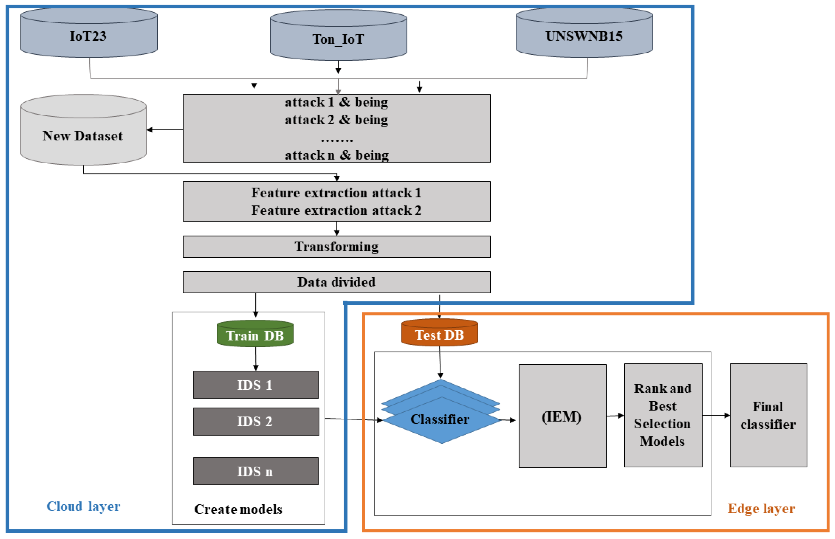
The proposed architecture is shown in Figure 1. The cloud layer contains different databases with different IoT network traffic. These databases are merged to generate a complex dataset used to create various machine and deep learning models using cloud resources. Once the models are created and trained using the training dataset, they will be placed on the edge layer for validation using the testing dataset on the Spark framework to obtain the model performance score. There are two separate phases; the first phase contains the integrated evaluation metrics (IEM) introduced in Section 5.1. The second phase contains the Rank and best selection method (RBSM), where all models will be ranked based on integrated evaluation metrics; the model with rank = 1 in all evaluation metrics means the model is the best and will be selected as part of the final classifier. The process of selection models is performed after the final and summation rank value are calculated. The model with the high final rank value or the model with a low summation rank value will be chosen to be a part of the final ensemble model. Our methodology is based on soft voting as it improves on hard voting.

5.1. Integrated Evaluation Metrics (IEM)

From the cybersecurity perspective, detecting attacks earlier is an essential aspect of any IDS. The detection time of the model plays a fundamental role in discovering and terminating the attack’s process without reducing the accuracy. For that purpose, time is required while simultaneously evaluating the model performance with model accuracy. We have integrated four evaluation metrics in our model, namely, F-score, Cohens Kappa, Matthew’s Correlation Coefficient (MCC), and logloss. In order to determine the performance of each suggested evaluation metric, we divide it by the detection time except for the logloss metric to obtain the efficiency score value. The high value of the efficiency score determines the most suitable model, and it is assigned with the high rank as ${\mathrm{metric}}_i=1$ where $i=\mathrm{F}-\mathrm{measure},\mathrm{Kappa},\mathrm{MCC},$ and $\mathrm{logloss}$.

• The efficiency score value of F-measure: It considers both precision and recall [43]. A more suitable model has a greater efficiency value based on Equation (1).

  $$\mathrm{The}\mathrm{efficiency}\mathrm{score}\mathrm{value}\mathrm{of}\mathrm{F}-\mathrm{measure}=\frac{\mathrm{F}-\mathrm{measure}}{\mathrm{Detection}\mathrm{time}}$$

  (1)
• The efficiency score value of Kappa: Cohens Kappa was first proposed to measure psychological behaviour observers’ agreement. It was designed to evaluate the degree of agreement or disagreement between two or more persons who were viewing the same phenomena [44]. The higher Kappa value should be assigned to the better-performing model using Equation (2).

  $$\mathrm{The}\mathrm{efficiency}\mathrm{score}\mathrm{value}\mathrm{of}\mathrm{Kappa}=\frac{\mathrm{Kappa}}{\mathrm{Detection}\mathrm{time}}$$

  (2)
• The efficiency score value of Matthew’s Correlation Coefficient (MCC): Is a technique used for evaluate model ability in both binary and multi-class classification. The MCC value is always between −1 and +1, where −1 indicating perfect misclassification and +1 indicating perfect classification [45]. The higher value MCC should be assigned to the better-performing model using Equation (3).

  $$\mathrm{The}\mathrm{efficiency}\mathrm{score}\mathrm{value}\mathrm{of}\mathrm{MCC}=\frac{\mathrm{MCC}}{\mathrm{Detection}\mathrm{time}}$$

  (3)
• The efficiency score value of logloss: Logloss is the most critical classification metric. It is based on probabilities, and it is used for comparing models and can be calculated as shown in Equation (4) [46]. The Lower logloss should be assigned to the better-performing model. Therefore we will sort this value by descending order.

  $$\mathrm{The}\mathrm{efficiency}\mathrm{score}\mathrm{value}\mathrm{of}\mathrm{Logloss}=-\frac{1}{N}\sum _{i=1}^N{y}_i.log\left(p\left(y_i\right)\right)+(1-y_i).log(1-p\left(y_i\right)).$$

  (4)
  Each metric will be ranked based on the obtained efficiency value. Then the rank will be used to determine the model performance score using the Spark big data processing system.
• The model performance score: We proposed the new equation to determine the Spark system’s best model performance for our scenarios. The equation has two parts. The first part is the summation of the model rank (r) of all metrics (F-measure, Kappa, MCC, and 2 × logloss). The second part is the time of the model to process all datasets using Spark. All models will be ranked based on time to process all datasets as $mode{l}_i$ rank = 1, 2, …, N where i = name of the model and N = number of the model in the list. The model with rank (r) = 1 is considered the model with low processing time, as defined in Equation (5). A more suitable model has a low-summation value with low processing time.

  $$\mathrm{Model}\mathrm{performance}\mathrm{score}=\mathrm{F}\left(\mathrm{r}\right)+\mathrm{Kappa}\left(\mathrm{r}\right)+\mathrm{MCC}\left(\mathrm{r}\right)+2\times \left(\mathrm{Logloss}\right(\mathrm{r}\left)\right)+\mathrm{Process}\left(\mathrm{r}\right)$$

  (5)

5.2. Rank and Best Selection Method (RBSM)

To design an efficient IDS for an IoT heterogeneous environment, we need to enhance decision-making and work with various network features. The proposed model is fully automated and flexible to create a robustness ensemble classifier. The classifier consolidates the top high performance of the machine and deep learning models using (IEM) and detection time, taking into account the total time of the model to process all the datasets using Spark. All suggested models will be trained using Stratified k fold cross-validation technique on our merged dataset, as shown in Algorithm 1. During inference, the mean results of integrated evaluation metrics of every model on these 5-folds are stored in JSON files. The rank model will use this file.

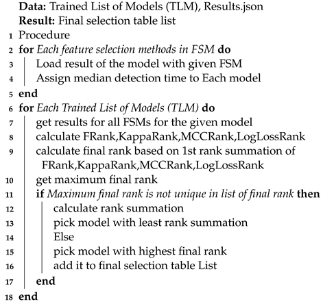
The detection time is an essential factor in utilizing the proposed integrated evaluation metrics. For this reason, the first step is to obtain the detection time per packet for each model. The second step is dividing all metrics by detection time to obtain the efficiency value of the metric to perform the ranking step except for the logloss metric. The model with a high value of logloss is identified as the worst model, and the model will be assigned with a low-rank. The strategy of the ranking algorithm is based on descending order, where the model with rank = 1 for each metric means more promising model than others. In our case, the ranking range is from (1 to 10) as our list contains ten machine/deep learning models. The proposed algorithm for the ranking model is presented in Algorithm 2.

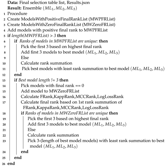
After the ranking step is performed, the best selection method will be performed using the final rank (FR) and summation rank (SR). All metrics ranked with ones will be added to obtain the final rank. On the other hand, the summation rank can be found by accumulating all metrics rank. The proposed algorithm for the best selection method is presented in Algorithm 3. The final (FR) and summation rank (SR) values are essential to perform the best selection method. The proposed ensemble classifier required three different models. To accomplish this task, the best selection method has two different cases that can appear and need to be addressed to ensure that our algorithm is performing in the best way. In the first case, three or more models are found after the final rank is added. In this case, the best selection method will choose the model with the final rank’s high value. In the second case, less than three models are found after adding the final rank. In this case, the best selection method will choose the model with the summation rank’s low value to be sure the algorithm is accurate and has selected the best model. Moreover, the proposed model will automatically update the ensemble classifier to meet the IoT traffic heterogeneity in the case of changing IoT networks. A detailed explanation is shown in the result section.

Algorithm 1: Training list of models using 5 Folds.

Algorithm 2: Ranking Algorithm.

Algorithm 3: Best Selection Algorithm.

6. Methodology

This section provides an overview of the selection, processing of the datasets, the machine learning models and the inference process. From the three original datasets (UNSW-NB15, Aposemat IoT-23, ToN_IoT), a number of data preparation techniques have to be carried out to make the datasets more useable. This section discusses the steps for the preparation of data before it was fed to the machine learning algorithms.

6.1. Datasets Description

Three publicly available datasets that contain a massive number of traffics, the UNSW-NB15 dataset, Aposemat IoT-23 dataset, and the ToN_IoT dataset, are used to evaluate the proposed approach, as shown in

Table 2. Abstract information of each dataset.

Information	UNSW-NB15	IoT23	ToN_IoT
Normal	2,218,764	30,858,735	300,000
Anomaly	321,283	294,449,255	161,043
Total	2,540,047	325,307,990	461,043
Number of features	49	23	45
Number Attack	9	14	9
Year of publication	2015	2020	2020
Number of IoT devices	-	3	9

.

The UNSW-NB15 dataset [47] contains a gigantic network traffics. There are more than two million abnormal and normal connection records. This dataset is high-dimensional with 49 features for each connection record and an average velocity of 5–10 MBs, reflecting real-world environments. Even though the UNSW-NB15 dataset is old, it still includes patterns of recent nine types of attacks, namely, Fuzzers, Analysis, Backdoors, DoS, Exploits, Generic, Reconnaissance, Shellcode and Worms and it is one of the most extensively used benchmark datasets for evaluating IDS.

Aposemat IoT-23 [48] is the recent dataset available on the issue of IoT traffics and network monitoring. The dataset includes 325,307,990 captures, of which 294,449,255 are malicious. The IoT traffic recorded by Aposemat IoT-23 comes from real hardware IoT devices (a Philips HUE smart LED lamp, an Amazon Echo home intelligent personal assistant, and a Somfy Smart Door Lock). Twenty captures of malware launched in IoT devices and three captures of benign IoT device data were acquired as part of the stratospheric project. Various botnets, including Mirai and Torii, were used in the attacks.

In an IoT domain, ToN_IoT is the most recent dataset developed by [18], and contains real traffic from recent attacks. It contains heterogeneous data sources such as IoT and IIoT sensor telemetry, Windows 7 and 10 operating system datasets, Ubuntu 14 and 18 TLS datasets, and network traffic datasets. The data came from a realistic and large-scale test-bed system founded at UNSW Canberra Cyber’s IoT Lab, which connected multiple virtual machines, physical systems, hacking platforms, cloud and fog platforms, and IoT sensors to simulate the complexity and scalability of IIoT and Industry 4.0 networks.

6.2. Dataset Integration

As a development, we integrate the most recent IoT datasets (Ton_IoT and IoT23) and the UNSW-NB15 dataset. The merged dataset will compare our technique against intrusion detection techniques proposed in the state-of-the-art. Several reasons are behind the merging of the datasets. For example, the problem of data imbalance, combining different samples for each class will reduce the effect of the data imbalance problem. Furthermore, the UNSW-NB15 dataset provides data on local traffic, while Aposemat IoT-23 and the ToN_IoT datasets contain data about real-time IoT traffic. On separated datasets, machine learning algorithms are usually preferably suitable. However, merging all datasets will create a complex dataset including real-IoT traffic and local traffic to examine the suggested approach’s performance.

6.3. Feature Selection Methods (FSMs)

Is a process used in machine learning to reduce the number of input features to improve model performance and reduce computation cost of using memory and CPU. This process can also be beneficial for simplifying models to make them easier to interpret and test the quality of the selected feature. Therefore, we utilized six methods for selection features including Kendall rank correlation coefficient, Spearman’s rank correlation coefficient, Pearson correlation coefficient, Chi-Square Test, Mutual Information, and ANOVA F-value (F-Class IF). The description for each one is as follows:

• Kendal: It is a statistical method that finds the ordinal correlation coefficient measurement value between two features in a non-parametric way [49];
• Spearman: It calculates a correlation or statistical measure between two continuous or ordinal features [50]. Instead of comparing raw data with ranked values, the Spearman correlation coefficient considers the rank of the variable;
• Pearson: It is a Correlation measures determine whether two continuous variables are linearly related. When one variable changes proportionally, it is a linear relationship [51];
• Mutual Information: It describes the statistical resemblance between two non-negative characteristics. MI equals zero if two independent features and higher values mean higher dependency [52];
• Chi-squared (Chi2): A non-parametric measure that evaluates the independence between two non-negative categorical variables features [53];
• ANOVA F-value (F): A technique for identifying how significantly two or more groups of quantitative features differ. By grouping a numerical feature by the target feature, this examines if the means of each group are significantly different. Low variances suggest that the target feature will not be affected and vice-versa [54].

To discover what works best for our specific problem, we chose to work with threshold 10%, 25%, 50%, 75%, 90% to select top features outputted from these techniques based on that threshold and created multiple instances of the original dataset with those features. In our paper, this process was divided into two sub-processes. First, we ranked our features using each feature selection method and selected top percentage features. The purpose is to make interpreting the model easier for the researcher and determine the dependability of the proposed detection models on different features while also considering the dynamic of IoT networks.

6.4. Dataset Preprocessing

One of the key ideas in our paper is to create a dataset that covers a wide range of attacks in networks using multiple datasets to create a unique model that knows this range of attacks so that we will not need multiple models specialized in every type of attack. The decision was to use all the three original datasets to construct the final merged dataset, which will be fed to the machine and deep learning algorithms. The merged dataset covers different families of attacks that could occur on any IoT network. The three datasets were chosen based on analysing the common features and covered practically all known attacks in networks. By common features, we mean that these datasets contain the same feature in terms of data/meaning but with different names in the dataset schema. The main problem with merging all three datasets is that these datasets have a variety number of features that will lead to samples values for non-shared features being nothing but NaN values. To solve this problem, we only picked the shared features. Preprocessing was performed on two different levels; on the first level, each dataset was preprocessed individually as follows:

• Cleaning the dataset by removing all features with zeros or no values where these features have no impact on classification;
• Reducing the number of features to the minimum number of features shared among all datasets. The features picked from IoT23 dataset features are [“id.orig_p”, “id.resp_p”,
  “proto”, “service”, “duration”, “orig_bytes”, “re sp_bytes”, “orig_pkts”, “resp_pkts”, “detailed-label”]. The features picke from ToN_IoT dataset are: [“src_port”, “dst_port”, “proto”, “service”, “duration”, “src_bytes”, “dst_ bytes”, “src_pkts”, “dst_pkts”, “type”].
  The features picked from UNSW-NB15 dataset are [“sport”, “dsport”, “proto”, “service”, “dur”, “sbytes”, “dbytes”, “Spkts”, “ Dpkts”, “attack_cat”].
  These are all shared features between the three datasets which contain same information along them but had only different names. For that reason, after creating the merged dataset, the features were renamed to [“id.orig_p”, “id.resp_p”, “proto”, “service”, “duration”, “orig_bytes”, “re sp_bytes”, “orig_pkts”, “resp_pkts”, “detailed-label”] to be usable in the training and testing phase;
• Removing redundant rows from the dataset reduces overfitting appearance and test model generalizability. Moreover, it enabled the reduction of the computational power required to train all the different machine learning algorithms.

After preprocessing each dataset individually, their outputs were used for concatenation in order to obtain the final dataset used in this research. On the second level, pre-processing was performed on the final dataset by:

• After merging all the datasets, the detailed-label (target feature) disposed of high imbalanced classes across the dataset with 32 types of attacks. In order to keep track of those different types of attacks and reduce the effect of data imbalance, we tried to merge similar types of attacks into one single class of attack. A detailed search about all these types of attacks was made to get them in their right classes; for instance, both C&C and C&C-FileDownload attacks can be merged into one type of attack called C&C. A device is infected with one of these types of attacks it can be ordered to perform various attacks in the future by sending a file to the device by the server. C&C-HeartBeat monitors the status of the infected device with small periodic messages sent by the server. C&C-HeartBeat-Attack is similar to previous attacks, but it is unclear how it is being carried out, only that this attack comes periodically from a suspicious source. A small file is sent instead of a data packet for the C&C-HeartBeat-FileDownload, to check the status of the device. For that reason, all previous types of attacks were merged into one class called C&C HeartBeat. Okiru and Okiru Attack types had been merged to one class named Okiru. Okiru is a more sophisticated version of the Mirai network. However, the Okiru Attack is the same as the previous one, but it is much more challenging to determine how and why the attack occurred. Part Of A Horizontal Port Scan, Part Of A Horizontal Port Scan-Attack, and C&C Part Of A Horizontal Port Scan are designed to gather information for future attacks by sending packages of data over the network. These types of attacks are combined in one class named Port Scan [55]. After this process, we have obtained 19 different classes of attack, as shown in

  Table 3. Attack classes and type.

  Attack Class	Type	No. Records	Class Encoding
  Normal	Benign	22,000	0
  	Normal
  C&C	C&C	11,268	1
  	C&C-FileDownload
  C&C HeartBeat	C&C-HeartBeat	21,206	2
  	C&C-HeartBeat-Attack
  	C&C-HeartBeat-FileDownload
  Mirai	Mirai	2	3
  Torii	Torii	16	4
  DoS	DDoS	22,000	5
  	Dos
  	Mitm
  	Fuzzers
  FileDownload	FileDownload	18	6
  Okiru	Okiru	15,324	7
  	Okiru-Attack
  Port Scan	Part of A Horizontal Port Scan-Attack	22,000	8
  	Part of A Horizontal Port Scan Analysis
  	Scanning
  	Analysis
  	Reconnaissance
  Attack	Attack	9398	9
  Ransomware	ransomware	3016	10
  Backdoor	backdoor	21,030	11
  Exploits	Exploits	22,000	12
  Generic	Generic	22,000	13
  Worms	Worms	174	14
  injection	injection	19,898	15
  xss	xss	14,151	16
  password	password	19,839	17
  Shellcode	Shellcode	1511	18

  . Random undersampling was applied to the majority type as a second technique used to reduce the effect of highly imbalanced samples in each class.
• In the merging dataset there are three categorical features, namely, “Service”, “Proto”, and “Detailledlabel”. These feature need to be encoding to be used in the training and testing phase as follow:
  The “Service” feature has 17 different categories, which through visualization were divided into two parts, highly used services, a lowly proportion for other categories and NaN values. This feature was encoded using nominal encoding since no notion of order exists here between categories.

  Table 4. Service Feature.

  Category	No. Records	Feature Encoding
  NaN values and lowly presented categories	166,250	0
  DNS	25,973	1
  HTTP	42,185	2
  FTP	3605	3
  SMTP	2324	4
  SSH	6514	5

  presents how the categories of this feature were encoded.
  The feature “proto” contains 131 different categories. Through visualization, categories were divided into three groups TCP, UDP, and other protocols. The TCP and UDP were highly used in the dataset, where other protocols were lowly used.

  Table 5. Proto Feature.

  Category	No. Records	Feature Encoding
  TCP	207,214	0
  UDP	29,086	1
  NaN values and lowly presented categories	10,551	2

  presents how the categories of this feature were encoded.
  After these steps, a final deleting of duplicate rows was performed as this step was initially conducted on each dataset individually, so we need to assert that after merging datasets, no duplicate rows are presented in the final dataset.
• Numerical data in the dataset differs in ranges, making compensating for these differences challenging to the classifier during training. In order to provide more homogeneous values to the classifier, it is essential to normalize the values in each attribute so that the minimum value is zero and the maximum is one.

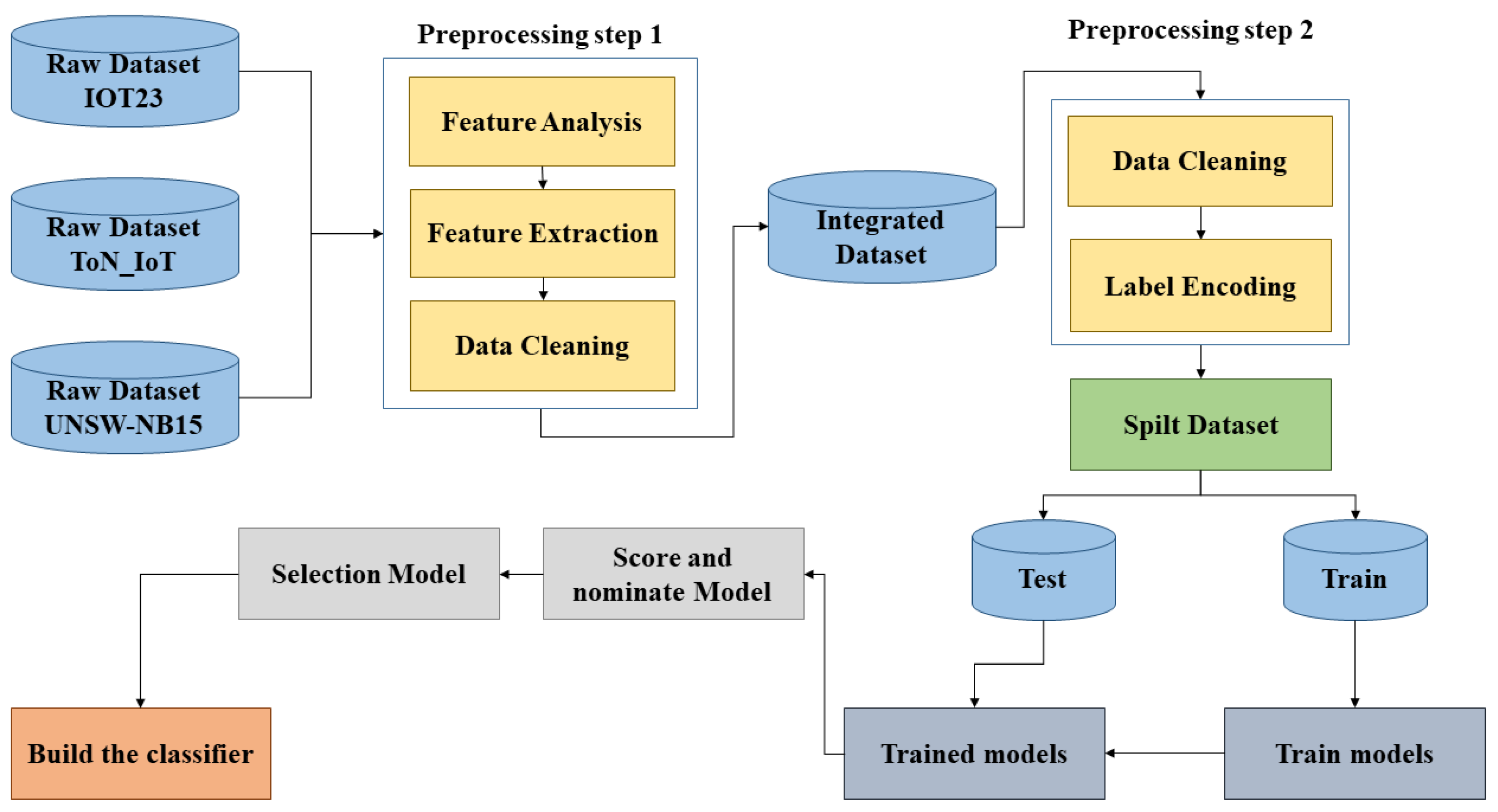
The pre-processing, data preparation and data integration are highlighted in Figure 2.

6.5. Applying Machine Learning Models and Ensemble Techniques for Classification

In this paper, we have trained ten different machine and deep learning models. Hyperparameters for all the models are the same for binary and multi-class approaches to avoid biased results toward one approach when tuning these hyperparameters.

Table 6. Model Hyperparameters sitting.

Model	Hyperparameters
RF	n_estimators = 100, criterion = ‘gini’
AdaBoost	n_estimators = 100, criterion = ‘gini’
DT	criterion = ‘gini’, splitter = ‘best’
KNN	n_neighbors = 5, leaf_size = 30, p = 2,
	metric = ‘minkowski’
Naive Bayes	var_smoothing = 1 × 10−9
LightGBM	boosting_type = ‘gbdt’, num_leaves = 31,
	max_depth = −1, learning_rate = 0.1, n_estimators = 100
CatBoost	n_estimators = 100, Learning_rate = 0.28,
	depth = 6 , loss_ f unction:
	MultiClass, max_leaves: 64
ANN	num_classes = 2 if binary else num_classes = 19 for multiclass
	activation = “sigmoid” if binary else “softmax” clf = Sequential()
	clf.add (Dense (units = 128, input_dim = 9, activation = ‘relu’))
	clf.add (Dropout (0.2)) clf.add (Dense (units = 256, activation = ‘relu’))
	clf.add (Dropout (0.2)) clf.add (Dense (units = 256,
	activation = ‘relu’)) clf.add (Dropout (0.2))
	clf.add (Dense (units = 128, activation = ‘relu’)) clf.add (Dropout (0.2))
	clf.add (Dense (units = num_classes, activation = activation))
CNN	activation = “sigmoid” if binary else “softmax”
	clf.add (Conv2D (filters = 32, kernel_size = (1,3),
	input_shape = (1,9,1), padding = ‘same’, activation = ‘relu’))
	clf.add (Conv2D (filters = 32, kernel_size = (1,3), padding = ‘same’,
	activation = ‘relu’)) clf.add (MaxPool2D (pool_size = (1,2))) clf.add (Flatten())
	clf.add (Dense (units = 256, activation = ‘relu’)) clf.add (Dropout (0.2))
	clf.add (Dense (units = 512, activation = ‘relu’)) clf.add (Dropout (0.2))
	clf.add (Dense(units = num_classes, activation = activation))
LSTM	num_classes = 2 if binary
	else num_classes = 19 for multiclass activation = “sigmoid”
	if binary else “softmax” clf.add (LSTM (units = 60,
	return_sequences = True, input_shape = (1,9))) clf.add (Dropout (0.2))
	clf.add (LSTM (units = 120, return_sequences = True)) clf.add (Dropout (0.2))
	clf.add (LSTM (units = 120)) clf.add (Dropout (0.2))
	clf.add (Dense (units = num_classes, activation = activation))

shows the hyperparameters for each model. There is a mix of models based on time series (LSTM), segmentation (CNN), non-linear (ANN), distances (KNN), Probabilities (Naive Bayes), Bagging (RandomForestClassifier), Boosting algorithms (LightGBM, CatBoostClassifier, AdaBoostClassifier), and basic decision tree model as shown in Figure 3. The training step is performed using 5 StratifiedKFold on our merged dataset, as shown in Algorithm 1. The mean results of each model on these 5 Folds from each feature selection method are stored in JSON files during inference. We will load these results and apply our procedure to achieve the best models. When starting to create our models we noticed that models with low-feature space have a low detection time in order to encounter this space-time trade-off, and in order to achieve non-biased results, we assigned each model detection time as the median of all its detection times with any set of features or all FSM used during training and inference.

As shown in Figure 4, three different models will be used to construct our proposed approach model. The three models’ decisions will be combined with weighted average ensembling in this research. Weighted average ensembling combines models’ outputs giving a weight to each of them. Those weights need to sum up to 1 as Equation (6).

$$FinalPrediction=P\left(M1\right)\times \alpha +P\left(M2\right)\times \gamma +P\left(M3\right)\times \beta \mathrm{where}\alpha +\gamma +\beta =1.$$

(6)

7. Evaluation’s Approach

This section provides the details of experimental environment setup, evaluation metrics, and the performance analysis for our proposed ensemble approach.

7.1. Experimental Details

Experiments were conducted on the Google Colab Pro + Platform [56]. This research used the scikit-learn, catboost and lightgbm packages for feature selection methods and models implementation and pandas for the data preprocessing [57]. The merged dataset was divided into 80% for training and 20% for testing using the 5-folds cross-validation process. The random seed is used for the Stratified K Fold function to produce distinct and various datasets for training and testing in each iteration of cross-validation, maintaining the same percentage of target labels in the training and testing set to have accurate results for all classes when evaluating our models. The next step is testing the models on the Spark processing platform in order to validate the model processing time on all records in the merged dataset. For this step, the experiment was performed on a local desktop computer (64-bit, 16 GB RAM, Core I7). The software stack contained Java (JDK) 11, Hadoop 2.7, Spark v3.0, and Pyspark 3.0.

7.2. The Evaluation Metrics

The metrics used to evaluate the performance of our models were logloss Equation (4), weighted F1-Score for multi-classification, F1-Score for binary classification, Accuracy, Kappa, Matthews_corrcoef, Recall, and Precision. We have also included processing time as a part of our metrics because time in IoT systems is crucial and we need models to have shorter processing time with a high level performance. The following are the techniques used to evaluate the model:

• 1-Recall: It is another metric that knows also as sensitivity or true positive rate. It measures the proportion of real positive instances that have been predicted positive [58]. Recall can be calculated using the Equation (7).

  $$Recall\left(Re\right)=\frac{TP}{TP+FN}.$$

  (7)
• 2-Precision: Precision is also called predictive values; it refers to the proportion of predicted positive and negative results that are true positive and true negative results, respectively. Precision is applied to a variety of areas to describe the performance model such as machine learning, data mining, and information retrieval [58]. Precision can be calculated using Equation (8).

  $$Precision\left(Pr\right)=\frac{TP}{TP+FP}.$$

  (8)
• 3-Accuracy: Accuracy can be explained as the overall performance of the classification model [59]. Accuracy can be calculated using Equation (9).

  $$Accuracy=\frac{(TP+TN)}{TP+FP+TN+FN}.$$

  (9)
• 4-Matthew’s Correlation Coefficient (MCC): Is a technique used for evaluate binary classifications and multi-class classification. The MCC value is always between −1 and +1, where +1 denotes indicating perfect positive correlation and −1, representing perfect negative correlation [45]. The MCC can be calculated using Equation (10).

  $$MCC=\frac{(TP\times TN-FP\times FN)}{\sqrt{(TP+FP)(TP+FN)(TN+FP)(TN+FN)}}.$$

  (10)
• 5-Cohen’s Kappa: It is a technique used to measure the extent to which two rates or judges agree on the classification of samples. Kappa can be calculated using Equation (11).

  $$k=\frac{(p_o-p_e)}{(1-p_e)},$$

  (11)

  where: $p_o$: The level of agreement observable among raters and $p_e$: Probabilities of chance agreement hypothesized.
• 6-Weighted F1-Score: Known also as F-measure considers both precision and recall. Weighted F1-score can be calculated using the Equation (12) [43]. This equation will be used for multi-classification scenario.

  $$\begin{array}{c}\mathrm{F}1-\mathrm{score}={\displaystyle \sum _{i=1}^C}\frac{Clas{s}_i}{N_i}\times F_{clas{s}_i}.\end{array}$$

  (12)
• 7-F1-Score: For binary classification scenario, we will use Equation (13)

  $$\mathrm{F}1=2\times \frac{(precision\times recall)}{precision+recall}.$$

  (13)
• 8-Processing time: It refers to the number of results produced per unit of time.

7.3. Experimental Results

As shown,

Table 7. Ranking of detection model using the Merged dataset for binary classification.

	Model	F-Measure	Rank	MCC	Rank	Kappa	Rank	Logloss	Rank	RT	FR	SR
1	RF	0.99518	5	0.99036	5	0.99036	5	0.018427	2	1.19 × 10−5	0	17
2	AdaBoost	0.99509	6	0.99018	6	0.99018	6	0.019059	3	6.57 × 10−5	0	21
3	DT	0.99304	1	0.98609	1	0.98609	1	0.21675	7	3.61 × 10−7	3	10
4	KNN	0.99122	7	0.98245	7	0.98245	7	0.12366	5	18.29 × 10−5	0	26
5	Naive Bayes	0.70103	2	0.27372	3	0.15750	3	1.52670	9	3.01 × 10−7	0	17
6	LightGBM	0.99445	4	0.98891	4	0.98890	4	0.015542	1	3.81 × 10−6	1	13
7	CatBoost	0.99039	3	0.98077	2	0.98077	2	0.03110	4	4.58 × 10−7	0	11
8	ANN	0.92130	9	0.85025	9	0.84795	9	2.6257	10	0.00034	0	37
9	CNN	0.94371	10	0.89012	10	0.88931	10	0.18933	6	0.00061	0	36
10	LSTM	0.91824	8	0.84692	8	0.84363	8	0.28430	8	0.00023	0	32

contains four evaluation metrics named F-Score, MCC, Kappa, and logloss, respectively. Each metrics concatenates with a specific column called (Rank). The rank column is stored in descending order after dividing the value of each metric by Detection time (DT), as this factor plays an essential role in evaluating attack detection performance. On the other hand, the logloss metric is stored in upwards order only and gives a high rank to model with a high logloss value. The 1st Rank of each metric means the model is suitable. Table 7 presents the rank of the all models in the binary classification scenario. To compute the efficiency value of each metric for each model, we conduct and run our ranking Algorithms to find the Final Rank (FR) column, which will be used to select the best three models. As a result, three efficiency metrics, F-score, MCC, and Kappa, select the Decision Tree (DT) model and only one efficiency metric, logloss, determines the LightGBM model. Based on the Final Rank (FR) result, there are no more models to be selected. However, the ensemble classifier must contain three models; consequently, the algorithm computed the Summation Rank (SR), where all efficiency values are cumulative and stored. The next step is choosing the model with a low summation rank to be a part of the ensemble classifier, and the result shows that the CatBoost model received (11) in the summation rank.

The ranking algorithm computed the merged dataset’s efficiency values of each metric for each model to select the best three models for the multi-classification scenario.

Table 8. Ranking of detection model using the Merged dataset for Multi-classification.

	Model	F-Measure	Rank	MCC	Rank	Kappa	Rank	Logloss	Rank	RT	FR	SR
1	RF	0.97814	4	0.97625	4	0.97615	4	0.12043	2	1.44 × 10−5	0	14
2	AdaBoost	0.97754	6	0.97565	6	0.97554	6	0.13101	3	8.87 × 10−5	0	21
3	DT	0.97224	1	0.96980	1	0.96974	1	0.68280	8	1.93 × 10−7	3	11
4	KNN	0.89903	7	0.89568	7	0.89459	7	2.3847	9	9.16 × 10−5	0	30
5	Naive Bayes	0.31040	3	0.30337	3	0.28553	3	3.1111	10	7.05 × 10−7	0	19
6	LightGBM	0.97125	5	0.96821	5	0.96810	5	0.27611	4	1.64 × 10−5	0	19
7	CatBoost	0.97038	2	0.96801	2	0.96788	2	0.097418	1	1.08 × 10−6	1	7
8	ANN	0.78103	10	0.77662	10	0.77302	10	0.58418	7	0.00031	0	37
9	CNN	0.85985	9	0.86103	9	0.85816	9	0.32072	5	0.00022	0	32
10	LSTM	0.79692	8	0.79483	8	0.79198	8	0.51764	6	0.00018	0	30

presents the efficiency value of the models; as a result, three efficiency metrics, F-score, MCC, and Kappa, select the Decision Tree (DT) model and only one efficiency metric, logloss, choose the CatBoost model. Likewise, the Final Rank (FR) result shows that there are no more models to be selected. Therefore, no additional investigation is needed. However, the ensemble classifier must contain three models; thus, the algorithm used the Summation Rank (SR). The next step is choosing the model with a low summation rank to be a part of the ensemble classifier, and the result shows that the Random forest model received (14) in the summation rank.

Table 9. Final selected models for binary and multi-classification.

Dataset	Selected Models for Binary	FR	SR	Selected Models for Multi	FR	SR
Merged dataset	LightGBM	1	13	DT	3	11
	DT	3	10	RF	0	14
	CatBoost	0	11	CatBoost	1	7

is the summary of the final models selected for each binary and multi-classification scenario using a merged dataset. Interestingly, the Rank and Best Selection Model (RBSM) picked CatBoost and DT models for both scenarios. However, the Naive Bayes model in this research gained a high rank, as shown in Table 7 and Table 8, respectively, where in reality, the model’s performance is poor. The reason behind this is that the model has a very low response time compared to others, and when we divide, for example, the F score by the response time, the model will receive a high rank. However, it proves that our Integrated Evaluation Metrics (IEM) works perfectly, and such models will be eliminated to be chosen by the Best Models Selection (BSM).

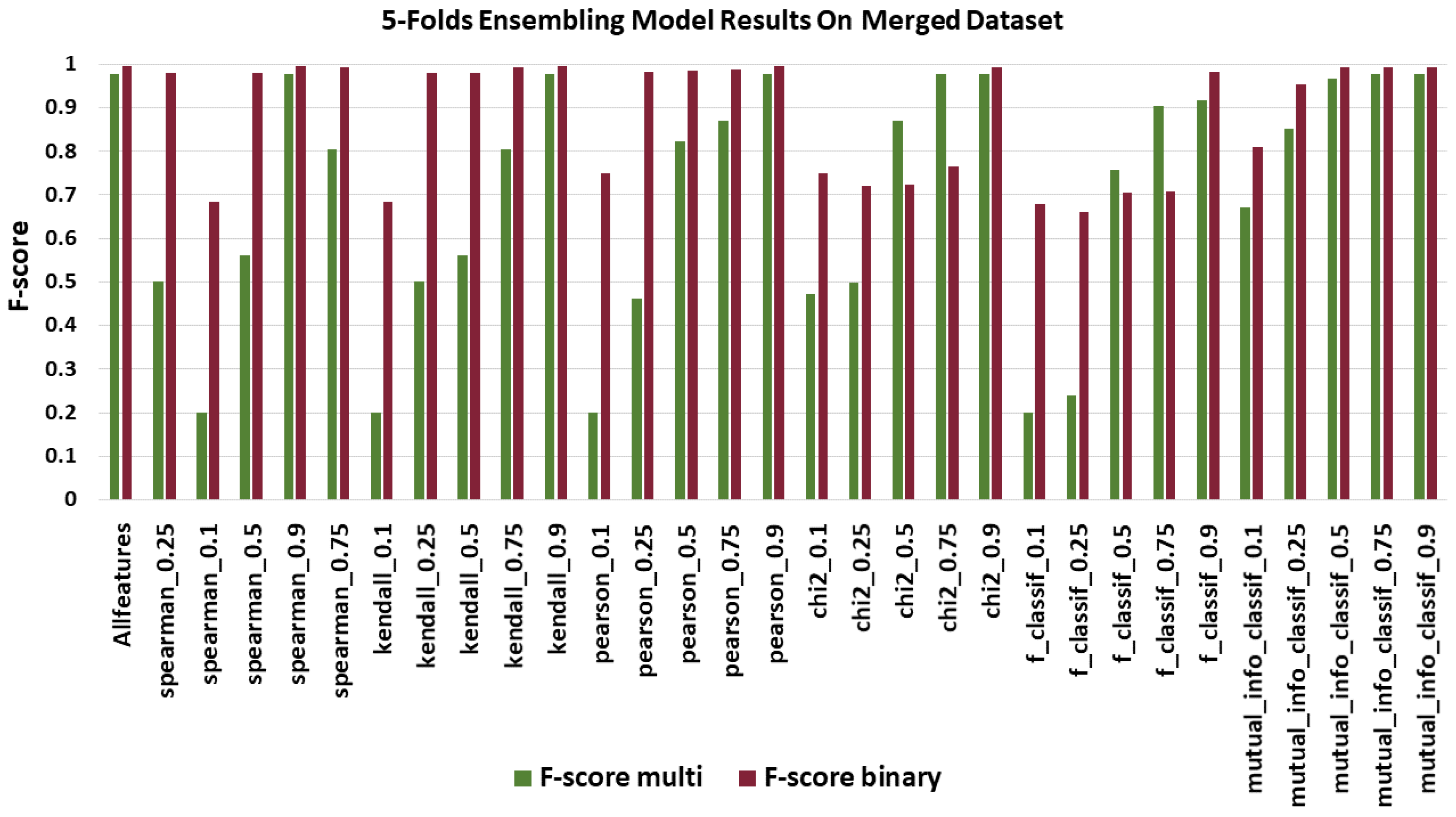
Figure 5, Figure 6, Figure 7, Figure 8 and Figure 9 present the Accuracy, F-score, MCC score, Kappa score, and logloss score for proposed model using FSMs in both binary and multi-classification scenarios. Figure 5 shows the weighted-average F1 Score of our ensembling model on the merged dataset. Our ensembling model did not show close results for each FSM as the weighted-average F1 Score ranges from 0.2 to 0.9782 for multi-classification. The model showed low scores when using a low-space features such as spearman_0.1, kendall_0.1, pearson_0.1 and f_classif_0.1 except for chi2_0.1 and mutual_info_classif_0.1 where the model showed average results. However, in binary classification F1 Score ranges from 0.689 to 0.994, where the model showed better performance even with the low-space feature. The model beat results with all features in the merged dataset using FSM. The best results were obtained with Pearson FSM with 90% of features from the full feature set in the merged dataset. These features were selected based on the Pearson correlation coefficient, so in this case, we have taken the first 90% of features with the highest Pearson correlation coefficient.

Figure 6 shows the accuracy score of the ensembling model on the merged dataset. In binary classification, accuracy ranges from 0.587 to 0.994, where the model showed better performance even with the low-space feature except for f1classif_0.1 in multi-classification, we can obtain that the model used the pearson_0.9 feature selection method on top of all other models with accuracy = 0.9781 as maximum accuracy score. Additionally, models trained with low-feature spaces presented poor results with accuracy near 0.28 except for chi2_0.1 and mutual_info_classif_0.1, which confirm that these feature selection methods selected the best possible set of features. For models with medium-feature spaces, they showed average results.

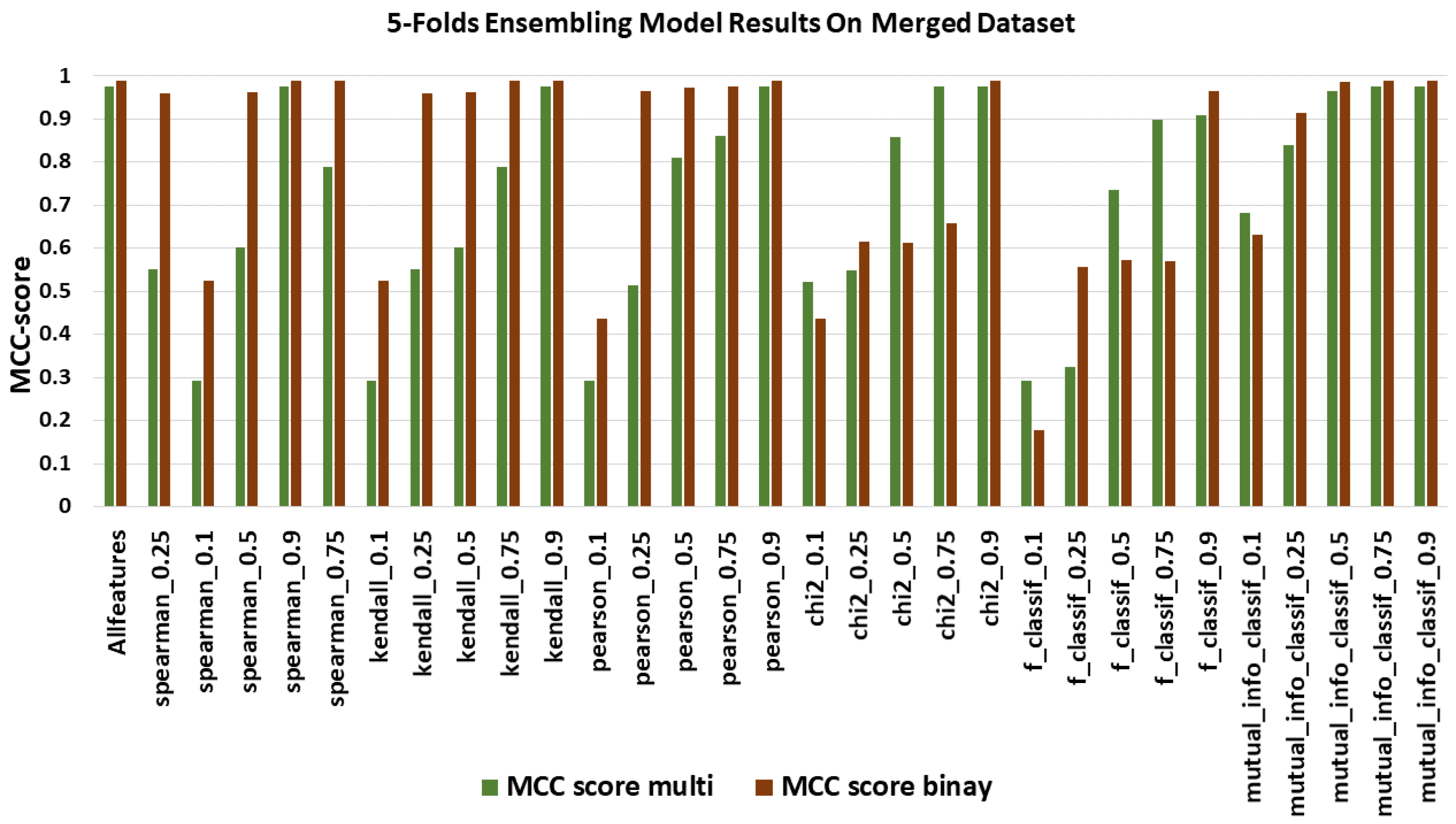
In terms of MCC Score, results correlate with the two previous figures and models with an important number of features that presented the highest scores. In Figure 7, the MCC Score for all feature selection methods ranged from 0.29 to 0.9763 multi-classification and 0.2 to 0.9945 for binary classification.

Figure 8 shows the Kappa score, ranging from 0.21 to 0.9762 multi-classification and 0.2 to 99.45 for binary classification. The model with the best Kappa score was an ensemble of three models with the same feature selection method applied, again the pearson_0.9.

In Figure 9, we can notice the exact opposite results of all previous figures as logloss is indicative of how close our prediction probabilities are to the actual value. logloss ranged from 1.95 to 0.072 for multi-classification. In binary classification, the range is 0.54 to 0.16, which is better than in multi-classification. The model with the most negligible logloss value was using the pearson_0.9 feature selection method.

In order to identify the best model performance, the models were examined utilizing Spark to process all datasets as we mentioned in Equation (5). The model performance contained the sum of all metrics and the model processing time of all datasets. From Figure 10, we can observe that the best processing time is obtained by the catboost model for multi-classification, whereas in binary classification, the Naive Bayes model is the best. However, based on Equation (5), Naive Bayes will be eliminated from the top three models.

Table 10. Model performance for binary classification.

	Models	F (r)	MCC (r)	Kappa (r)	Logloss (r)	Processing (r)	Sum	Model Score
1	RF	5	5	5	4	6	25	3
2	AdaBoost	6	6	6	6	7	31	5
3	DT	1	1	1	14	2	19	2
4	KNN	7	7	7	10	8	39	6
5	Naive Bayes	2	3	3	18	1	27	4
6	LightGBM	4	4	4	2	5	19	2
7	CatBoost	3	2	2	8	3	18	1
8	ANN	9	9	9	20	10	57	9
9	CNN	10	10	10	12	11	53	8
10	LSTM	8	8	8	16	9	49	7

and

Table 11. Model performance for multi-classification.

	Models	F (r)	MCC (r)	Kappa (r)	Logloss (r)	Processing (r)	Sum	Model Score
1	RF	4	4	4	4	6	22	2
2	AdaBoost	6	6	6	6	7	31	4
3	DT	1	1	1	16	3	22	2
4	KNN	7	7	7	18	7	46	6
5	Naive Bayes	3	3	3	20	2	31	4
6	LightGBM	5	5	5	8	5	28	3
7	CatBoost	2	2	2	2	1	9	1
8	ANN	10	10	10	14	10	54	7
9	CNN	9	9	9	10	9	46	6
	LSTM	8	8	8	12	8	44	5

show the performance results for all models. Notably, classifiers based on deep learning suffer from a significant drawback as such models consume large amounts of processing time. It becomes more problematic in real-time IDS, where attacker behaviour changes rapidly. In Section 3, several studies use deep learning without much consideration of processing time.

7.4. Comparison with State-of-the-Art Approaches

The proposed model’s performance is compared to various state-of-the-art methods that utilize the same datasets. The proposed ensemble classier performs sufficiently with the highest accuracy on merged datasets compared to previous studies. Moreover, all approaches presented used one or two datasets separately, and most of the studies’ experiments on the multi-classification dataset were not performed, none of them considering the processing time of models using a big data processing platform. With this consideration, the experiments conducted in this paper prove advantageous in realizing machine learning model performance on binary and multi-classification datasets using Spark. Furthermore, it demonstrates the proposed model’s improved performance in terms of binary and multi-class performances in heterogeneous IoT networks.

The proposed model’s performance is accurate for both scenarios, i.e., binary and multi-classification.

Table 12. State- of-the-Art Comparison.

Dataset	Reference	ACC	F-Score	MCC	Logloss	Kappa	Re	Pr	DT	PT
UNSW-NB15	Moustafa [13]	98.97	-	-	-	-	97.02	-	-	-
	Rashid [12]	94	-	-	-	-	-	-	-	-
	Zhou [8]	91.22	-	-	-	-	92.84	92.38	-	-
	Ahmad [11]	97.37	-	-	-	-	-	-	-	-
	Aleesa [7]	97.80	-	-	-	-	-	-	-	-
	Smitha [14]	94	95	-	-	-	93	96	-	-
IoT23	PuTianet [9]	89.5	90.15	-	-	-	84.45	96.82	-	-
	Amiya [16]	96	95.23	-	-	-	-	-	-	-
	Dutta [15]	99.7	98	99	-	-	95	100	-	-
	Nukavarapu [10]	92	-	-	-	-	-	-	-	-
ToN_IoT	Alsaedi [18]	87	87	-	-	-	87	88	-	-
	Booij [17]	98.07	97.26	-	-	-	-	-	-	-
Merge	Proposed model (Binary)	99.45	99.45	98.90	0.016	98.90	99.50	99.38	1.54 × 10−6	0.37
	Proposed model (Multi)	97.81	97.82	97.63	0.073	97.62	97.80	97.92	5.22 × 10−6	1.25

compares our proposed model and relevant publications in terms of accuracy, utilizing the all used datasets. As shown in the UNSW-NB15 dataset, our model overcomes all other studies. However, even the study of [13] slightly overcame our model; the study has been carried out on individual datasets and does not concern the performance of the models in terms of the detection time using Spark. Significantly, the proposed model overcomes the studies of [9,10,18], using Aposemat IoT-23 and Ton_IoT datasets, respectively. Table 12 indicates that the study of [15] slightly overcomes the proposed model. Similarly, this study has not covered the multi-classification issue nor the performance of the models in terms of detection time. Moreover, the experience has been conducted on an individual dataset.

8. Conclusions and Discussion

IoT refers to the network of devices that can collect and share data with other devices on the network. The IoT network allows the control of devices remotely through the existing network infrastructure, which creates many opportunities for the seamless integration of computer-based systems. However, this will create many challenges as well, including a massive volume of data traffic that needs to be processed to make a decision in real-time to secure and detect attacks in such a complex network. Therefore, it is essential to design scalable, flexible, and reliable IDS to meet the IoT requirements. IDS models need to be evaluated in detection time and accuracy under a big data environment. However, even existing IDS can detect anomalies with higher accuracy; such models cannot detect attack types from different domains of data, leading to more investigation time for the system administrator to identify the attack type. The aim of this research to address limitations of current IDSs by analyzed and evaluated ten machine and deep learning models using FSMs. For this objective, experimentation is performed on a merged complex dataset of two IoT datasets and one local traffic dataset.

One significant role of ensemble learning is increasing the confidence in the model decision. For that purpose, Integrated Evaluation Metrics (IEM) was proposed utilizing five efficiency metrics: F-score, Kappa, MCC, logloss, and the model processing time of all datasets. Furthermore, a ranking and best selection method (RBSM) is presented to rank the efficiency value of all metrics for each model to build a scalable, flexible and reliable ensemble classifier that can automatically be adaptable in adding machine/deep learning models or any IoT network changes. Experimental results indicate that the model’s training time is less as they are deployed in the cloud. Moreover, the processing time is fast when deploying the model at the edge using Spark without compromising detection efficiency. On the other hand, the performance of the proposed ensemble classifier is outstanding compared to other models in several state-of-the-art methods. The model reaches an accuracy of 99.45% for binary classification and 97.81% for multi-class classification. This paper conducts experiments by merging three datasets. However, all experiments are conducted using an IoT dataset. Applying our approach to other types of data may substantially affect the results. Our future works plan to perform further experiments by merging the data from different fields and investigating the effectiveness of the proposed technique.

References

- Chopra, K.; Gupta, K.; Lambora, A. Future internet: The internet of things-a literature review. In Proceedings of the 2019 International Conference on Machine Learning, Big Data, Cloud and Parallel Computing (COMITCon), Faridabad, India, 14–16 February 2019; pp. 135–139. [Google Scholar]
- Apostol, I.; Preda, M.; Nila, C.; Bica, I. IoT Botnet Anomaly Detection Using Unsupervised Deep Learning. Electronics 2021, 10, 1876. [Google Scholar] [CrossRef]
- Levina, A.I.; Dubgorn, A.S.; Iliashenko, O.Y. Internet of things within the service architecture of intelligent transport systems. In Proceedings of the 2017 European Conference on Electrical Engineering and Computer Science (EECS), Bern, Switzerland, 17–19 November 2017; pp. 351–355. [Google Scholar]
- Ashraf, J.; Bakhshi, A.D.; Moustafa, N.; Khurshid, H.; Javed, A.; Beheshti, A. Novel Deep Learning-Enabled LSTM Autoencoder Architecture for Discovering Anomalous Events From Intelligent Transportation Systems. IEEE Trans. Intell. Transp. Syst. 2021, 22, 4507–4518. [Google Scholar] [CrossRef]
- Zhou, Z.H. Ensemble Methods: Foundations and Algorithms; CRC Press: Boca Raton, FL, USA, 2012. [Google Scholar]
- Kumari, S.; Kumar, D.; Mittal, M. An ensemble approach for classification and prediction of diabetes mellitus using soft voting classifier. Int. J. Cogn. Comput. Eng. 2021, 2, 40–46. [Google Scholar] [CrossRef]
- Aleesa, A.; Younis, M.; Mohammed, A.A.; Sahar, N. Deep-intrusion detection system with enhanced UNSW-NB15 dataset based on deep learning techniques. J. Eng. Sci. Technol. 2021, 16, 711–727. [Google Scholar]
- Zhou, Y.; Han, M.; Liu, L.; He, J.S.; Wang, Y. Deep learning approach for cyberattack detection. In Proceedings of the IEEE INFOCOM 2018-IEEE Conference on Computer Communications Workshops (INFOCOM WKSHPS), Honolulu, HI, USA, 15–19 April 2018; pp. 262–267. [Google Scholar]
- Tian, P.; Chen, Z.; Yu, W.; Liao, W. Towards Asynchronous Federated Learning Based Threat Detection: A DC-Adam Approach. Comput. Secur. 2021, 108, 102344. [Google Scholar] [CrossRef]
- Nukavarapu, S.K.; Nadeem, T. Securing Edge-based IoT Networks with Semi-Supervised GANs. In Proceedings of the 2021 IEEE International Conference on Pervasive Computing and Communications Workshops and other Affiliated Events (PerCom Workshops), Kassel, Germany, 22–26 March 2021; pp. 579–584. [Google Scholar]
- Ahmad, M.; Riaz, Q.; Zeeshan, M.; Tahir, H.; Haider, S.A.; Khan, M.S. Intrusion detection in internet of things using supervised machine learning based on application and transport layer features using UNSW-NB15 data-set. EURASIP J. Wirel. Commun. Netw. 2021, 2021, 10. [Google Scholar] [CrossRef]
- Rashid, M.; Kamruzzaman, J.; Imam, T.; Wibowo, S.; Gordon, S. A tree-based stacking ensemble technique with feature selection for network intrusion detection. Appl. Intell. 2022. [Google Scholar] [CrossRef]
- Moustafa, N.; Turnbull, B.; Choo, K.K.R. An ensemble intrusion detection technique based on proposed statistical flow features for protecting network traffic of internet of things. IEEE Internet Things J. 2018, 6, 4815–4830. [Google Scholar] [CrossRef]
- Rajagopal, S.; Kundapur, P.P.; Hareesha, K.S. A stacking ensemble for network intrusion detection using heterogeneous datasets. Secur. Commun. Netw. 2020, 2020, 4586875. [Google Scholar] [CrossRef] [Green Version]
- Dutta, V.; Choraś, M.; Pawlicki, M.; Kozik, R. A deep learning ensemble for network anomaly and cyber-attack detection. Sensors 2020, 20, 4583. [Google Scholar] [CrossRef]
- Sahu, A.K.; Sharma, S.; Tanveer, M.; Raja, R. Internet of Things attack detection using hybrid Deep Learning Model. Comput. Commun. 2021, 176, 146–154. [Google Scholar] [CrossRef]
- Booij, T.M.; Chiscop, I.; Meeuwissen, E.; Moustafa, N.; den Hartog, F.T. ToN_IoT: The Role of Heterogeneity and the Need for Standardization of Features and Attack Types in IoT Network Intrusion Datasets. IEEE Internet Things J. 2021, 9, 485–496. [Google Scholar] [CrossRef]
- Alsaedi, A.; Moustafa, N.; Tari, Z.; Mahmood, A.; Anwar, A. TON_IoT telemetry dataset: A new generation dataset of IoT and IIoT for data-driven intrusion detection systems. IEEE Access 2020, 8, 165130–165150. [Google Scholar] [CrossRef]
- Alghamdi, R.; Bellaiche, M. A Deep Intrusion Detection System in Lambda Architecture Based on Edge Cloud Computing for IoT. In Proceedings of the 2021 4th International Conference on Artificial Intelligence and Big Data (ICAIBD), Chengdu, China, 28–31 May 2021; pp. 561–566. [Google Scholar] [CrossRef]
- Zaharia, M.; Xin, R.S.; Wendell, P.; Das, T.; Armbrust, M.; Dave, A.; Meng, X.; Rosen, J.; Venkataraman, S.; Franklin, M.J.; et al. Apache spark: A unified engine for big data processing. Commun. ACM 2016, 59, 56–65. [Google Scholar] [CrossRef]
- Han, J.; Haihong, E.; Le, G.; Du, J. Survey on NoSQL database. In Proceedings of the 2011 6th International Conference on Pervasive Computing and Applications, Port Elizabeth, South Africa, 26–28 October 2011; pp. 363–366. [Google Scholar]
- Yang, J.; Qu, J.; Mi, Q.; Li, Q. A CNN-LSTM model for tailings dam risk prediction. IEEE Access 2020, 8, 206491–206502. [Google Scholar] [CrossRef]
- Agatonovic-Kustrin, S.; Beresford, R. Basic concepts of artificial neural network (ANN) modeling and its application in pharmaceutical research. J. Pharm. Biomed. Anal. 2000, 22, 717–727. [Google Scholar] [CrossRef]
- LeCun, Y.; Bottou, L.; Bengio, Y.; Haffner, P. Gradient-based learning applied to document recognition. Proc. IEEE 1998, 86, 2278–2324. [Google Scholar] [CrossRef] [Green Version]
- Lan, T.; Hu, H.; Jiang, C.; Yang, G.; Zhao, Z. A comparative study of decision tree, random forest, and convolutional neural network for spread-F identification. Adv. Space Res. 2020, 65, 2052–2061. [Google Scholar] [CrossRef]
- Aldweesh, A.; Derhab, A.; Emam, A.Z. Deep learning approaches for anomaly-based intrusion detection systems: A survey, taxonomy, and open issues. Knowl.-Based Syst. 2020, 189, 105124. [Google Scholar] [CrossRef]
- Belgiu, M.; Drăguţ, L. Random forest in remote sensing: A review of applications and future directions. ISPRS J. Photogramm. Remote Sens. 2016, 114, 24–31. [Google Scholar] [CrossRef]
- Schapire, R.E. Explaining adaboost. In Empirical Inference; Springer: Berlin/Heidelberg, Germany, 2013; pp. 37–52. [Google Scholar]
- Zhou, H.; Zhang, J.; Zhou, Y.; Guo, X.; Ma, Y. A feature selection algorithm of decision tree based on feature weight. Expert Syst. Appl. 2021, 164, 113842. [Google Scholar] [CrossRef]
- Boualouache, A.; Engel, T. A Survey on Machine Learning-based Misbehavior Detection Systems for 5G and Beyond Vehicular Networks. arXiv 2022, arXiv:2201.10500. [Google Scholar]
- Rish, I. An empirical study of the naive Bayes classifier. In IJCAI 2001 Workshop on Empirical Methods in Artificial Intelligence; IBM: New York, NY, USA, 2001; Volume 3, pp. 41–46. [Google Scholar]
- Fan, J.; Ma, X.; Wu, L.; Zhang, F.; Yu, X.; Zeng, W. Light Gradient Boosting Machine: An efficient soft computing model for estimating daily reference evapotranspiration with local and external meteorological data. Agric. Water Manag. 2019, 225, 105758. [Google Scholar] [CrossRef]
- Hancock, J.T.; Khoshgoftaar, T.M. CatBoost for big data: An interdisciplinary review. J. Big Data 2020, 7, 1–45. [Google Scholar] [CrossRef]
- Saha, A.; Subramanya, A.; Pirsiavash, H. Hidden trigger backdoor attacks. In Proceedings of the Thirty-Fourth AAAI Conference on Artificial Intelligence (AAAI-20), New York, NY, USA, 7–12 February 2020; Volume 34, pp. 11957–11965. [Google Scholar]
- Mukhopadhayay, I.; Polle, S.; Naskar, P. Simulation of denial of service (DoS) attack using matlab and xilinx. IOSR J. Comput. Eng. (IOSR-JCE) 2014, 16, 119–125. [Google Scholar] [CrossRef]
- Ali, O.; Cotae, P. Towards DoS/DDoS attack detection using artificial neural networks. In Proceedings of the 2018 9th IEEE Annual Ubiquitous Computing, Electronics & Mobile Communication Conference (UEMCON), New York, NY, USA, 8–10 November 2018; pp. 229–234. [Google Scholar]
- Alenezi, M.; Nadeem, M.; Asif, R. SQL injection attacks countermeasures assessments. Indones. J. Electr. Eng. Comput. Sci. 2021, 21, 1121–1131. [Google Scholar] [CrossRef]
- Conti, M.; Dragoni, N.; Lesyk, V. A survey of man in the middle attacks. IEEE Commun. Surv. Tutorials 2016, 18, 2027–2051. [Google Scholar] [CrossRef]
- Subangan, S.; Senthooran, V. Secure authentication mechanism for resistance to password attacks. In Proceedings of the 2019 19th International Conference on Advances in ICT for Emerging Regions (ICTer), Colombo, Sri Lanka, 2–5 September 2019; Volume 250, pp. 1–7. [Google Scholar]
- Maniath, S.; Ashok, A.; Poornachandran, P.; Sujadevi, V.; AU, P.S.; Jan, S. Deep learning LSTM based ransomware detection. In Proceedings of the 2017 Recent Developments in Control, Automation & Power Engineering (RDCAPE), Noida, India, 26–27 October 2017; pp. 442–446. [Google Scholar]
- Phase, E. Scanning and Enumeration Phase. In Constructing an Ethical Hacking Knowledge Base for Threat Awareness and Prevention; IGI Global: Hershey, PA, USA, 2019. [Google Scholar]
- Fang, Y.; Li, Y.; Liu, L.; Huang, C. DeepXSS: Cross site scripting detection based on deep learning. In Proceedings of the 2018 International Conference on Computing and Artificial Intelligence; Association for Computing Machinery: New York, NY, USA, 2018; pp. 47–51. [Google Scholar] [CrossRef]
- Marir, N.; Wang, H.; Feng, G.; Li, B.; Jia, M. Distributed abnormal behavior detection approach based on deep belief network and ensemble svm using spark. IEEE Access 2018, 6, 59657–59671. [Google Scholar] [CrossRef]
- Cohen, J. A coefficient of agreement for nominal scales. Educ. Psychol. Meas. 1960, 20, 37–46. [Google Scholar] [CrossRef]
- Matthews, B.W. Comparison of the predicted and observed secondary structure of T4 phage lysozyme. Biochim. Biophys. Acta (BBA)-Protein Struct. 1975, 405, 442–451. [Google Scholar] [CrossRef]
- Aggarwal, A.; Kasiviswanathan, S.; Xu, Z.; Feyisetan, O.; Teissier, N. Label inference attacks from logloss scores. In Proceedings of the International Conference on Machine Learning, PMLR, Virtual, 18–24 July 2021; pp. 120–129. [Google Scholar]
- Moustafa, N.; Slay, J. UNSW-NB15: A comprehensive dataset for network intrusion detection systems (UNSW-NB15 network dataset). In Proceedings of the 2015 Military Communications and Information Systems Conference (MilCIS), Canberra, ACT, Australia, 10–12 November 2015; pp. 1–6. [Google Scholar]
- A Labeled Dataset with Malicious and Benign IoT Network Traffic. (Version 1.0.0) [Data set]. 2020. Available online: https://zenodo.org/record/4743746#.YmjKONNBycw (accessed on 31 March 2022). [CrossRef]
- Abdi, H. The Kendall rank correlation coefficient. In Encyclopedia of Measurement and Statistics; Sage: Thousand Oaks, CA, USA, 2007; pp. 508–510. [Google Scholar]
- Li, H.; Cao, Y.; Su, L. Pythagorean fuzzy multi-criteria decision-making approach based on Spearman rank correlation coefficient. Soft Comput. 2022, 26, 3001–3012. [Google Scholar] [CrossRef]
- Pan, H.; You, X.; Liu, S.; Zhang, D. Pearson correlation coefficient-based pheromone refactoring mechanism for multi-colony ant colony optimization. Appl. Intell. 2021, 51, 752–774. [Google Scholar] [CrossRef]
- Haber, E.; Modersitzki, J. Beyond mutual information: A simple and robust alternative. In Bildverarbeitung für die Medizin 2005; Springer: Berlin/Heidelberg, Germany, 2005; pp. 350–354. [Google Scholar]
- King, T. A Guide to Chi-Squared Testing. Technometrics 1997, 39, 431. [Google Scholar] [CrossRef]
- Alizadeh, M.; Mousavi, S.E.; Beheshti, M.T.; Ostadi, A. Combination of Feature Selection and Hybrid Classifier as to Network Intrusion Detection System Adopting FA, GWO, and BAT Optimizers. In Proceedings of the 2021 7th International Conference on Signal Processing and Intelligent Systems (ICSPIS), Tehran, Iran, 29–30 December 2021; pp. 1–7. [Google Scholar]
- Stoian, N.A. Machine Learning for Anomaly detection In IoT Networks: Malware Analysis on the IoT-23 dataset. Bachelor’s Thesis, University of Twente, Enschede, The Netherlands, 2020. [Google Scholar]
- Google Colab. Available online: https://colab.research.google.com/ (accessed on 25 February 2022).
- Kramer, O. Scikit-learn. In Machine Learning for Evolution Strategies; Springer: Berlin/Heidelberg, Germany, 2016; pp. 45–53. [Google Scholar]
- Powers, D.M. Evaluation: From precision, recall and F-measure to ROC, informedness, markedness and correlation. J. Mach. Learn. Technol. 2011, 2, 37–63. [Google Scholar]
- Sokolova, M.; Lapalme, G. A systematic analysis of performance measures for classification tasks. Inf. Process. Manag. 2009, 45, 427–437. [Google Scholar] [CrossRef]