Article

Assessing Feature Representations for Instance-Based Cross-Domain Anomaly Detection in Cloud Services Univariate Time Series Data

1
ADAPT Research Centre, Trinity College Dublin, D02 W272 Dublin, Ireland
2
ADAPT Research Centre, Dublin City University, D09 RFK0 Dublin, Ireland
3
Huawei Research, D02 R156 Dublin, Ireland
4
ADAPT Research Centre, Technological University Dublin, D07 EWV4 Dublin, Ireland
*
Author to whom correspondence should be addressed.
These authors contributed equally to this work.
IoT 2022, 3(1), 123-144; https://doi.org/10.3390/iot3010008
Submission received: 7 December 2021 / Revised: 30 December 2021 / Accepted: 10 January 2022 / Published: 29 January 2022

Abstract

:
In this paper, we compare and assess the efficacy of a number of time-series instance feature representations for anomaly detection. To assess whether there are statistically significant differences between different feature representations for anomaly detection in a time series, we calculate and compare confidence intervals on the average performance of different feature sets across a number of different model types and cross-domain time-series datasets. Our results indicate that the catch22 time-series feature set augmented with features based on rolling mean and variance performs best on average, and that the difference in performance between this feature set and the next best feature set is statistically significant. Furthermore, our analysis of the features used by the most successful model indicates that features related to mean and variance are the most informative for anomaly detection. We also find that features based on model forecast errors are useful for anomaly detection for some but not all datasets.

1. Introduction

A time series is a set of data points that were collected and are indexed sequentially through time. Time series analysis can be applied to a wide range of data-generating processes, including data from sensors monitoring tides, stock prices, and medical applications such as monitoring for cardiac pathologies. There are range methods that can be applied, such as visualization, classification, and anomaly detection. This paper focuses on anomaly detection in cloud systems. Anomaly detection is the identification of rare events; these events could be indicative of critical failures in cloud systems. One area of increasing importance for time-series analysis is the maintenance of cloud services. Cloud services are often made up of many microservices, all of which can have different operating parameters. For these services, different KPIs can be tracked and provide real-time insights into the performance of the different micro-services within the system, for example, the amount of network traffic might be useful for a load balancer, while levels of disk I/O might be informative for a database. Consequently, these KPIs provide a basis for the early detection of problems in a system due to system failure, crashes, or surges in traffic. Early detection of problems in this way can allow engineers to address issues or scale systems in a timely manner.
Nielsen [1] distinguishes between four different types of computational model for time series analysis, namely, (i) statistical models (e.g., auto-regressive models, and moving averages); (ii) state-space models (e.g., kalman-filters, hidden markov models); (iii) machine learning methods (e.g., SVMs, tree based ensembles) applied to hand-engineered feature sets; and (iv) end-to-end deep learning methods (e.g., recurrent architectures, and convolutional networks). Statistical and state-space methods augmented with thresholds and rules can work well for anomaly detection on relatively stable KPIs where the thresholds can be tailored to normal operation parameters of the KPI being monitored [2]. However, it is difficult to set appropriate thresholds when there is significant variation within a KPI due to temporal or seasonal variation [3], or where there is significant variation across a set of KPIs that is being monitored as part of a cloud services infrastructure [4]. Focusing on machine-learning-based methods, both supervised [5,6] and unsupervised methods [7,8,9] for anomaly detection have been proposed. There is also a growing amount of research in applying deep learning methods to anomaly detection for time-series. Within the research on deep anomaly detection models, the majority of research has focused on unsupervised methods; this is because of the difficulties that deep supervised models can have in modelling imbalanced data, and because of the lack of available training data (see [10] for a recent overview of this work). However, despite this current trend towards unsupervised deep anomaly detection research, and following [4,11], we believe supervised approaches to anomaly detection are ultimately necessary in order to achieve the high levels of performance required to support critical cloud-based services. In particular, our long-term research goals are to develop highly-accurate supervised machine learning/deep learning approaches to anomaly detection that scale across multiple domains with minimal data labelling overhead. This points to the use of transfer learning and active learning methods in the final framework. However, as a first step in the development of a scalable framework for time-series anomaly detection in this paper, we report results from a set of experiments that were designed to assess the relative performance of different feature representations of time-series data points for the task of cross-domain anomaly detection for univariate time-series data; moreover, we will focus on the interaction between these features sets and transfer learning and active learning in later work. The contributions of this paper are as follows:
  • A comprehensive analysis of the multiple feature time-series feature sets for anomaly detection across a number of cross-domain time-series datasets;
  • Identifying a feature set that outperforms the other representations by a statistically significant margin on the task of cross-domain anomaly detection;
  • Elaborating feature importance in the top performing representation.
The rest of this paper is structured as follows: in Section 2, we review related work on feature representations for time-series analysis; in Section 3, we describe the set of features that we are considering under experiment; in Section 4, we describe our experimental design and in particular introduce the dataset and models types we use in the experiment and our use of confidence intervals as part of our experimental method for feature comparison; in Section 5, we present the experimental results; and in Section 7, we present our conclusions.

2. Related Work on Feature Engineering for Time-Series Analysis and Anomaly Detection

Feature engineering and selection can have significant impact on the performance of a data-driven model on a given task. Using appropriate features can reveal relevant underlying information in a domain. For example, in time-series analysis, features can reveal variance, seasonality, or deviations from observable trends. However, including irrelevant or redundant features in a representation can result in models overfitting the particularities of the training sample. Furthermore, features that may be useful in one time-series task may not be appropriate for another. For example, the use of a mean makes sense where a time-series is stationary (or at least ergodic) but is less meaningful when a time-series is non-stationary, and features such as max and min values may become unstable as the length of a time-series increases ([1], p. 242). Consequently, selecting an appropriate feature set for a task and domain is important, although this become more challenging in a cross-domain setting.
In an era of end-to-end deep learning, many data-driven projects often rely on the ability of deep networks to learn the appropriate representations for a task from the raw data [12]. However, as noted above, relatively little work has been done on supervised deep learning methods for anomaly detection in time-series data because of the data required for deep learning approaches and because of the difficulties of training deep models using highly-imbalanced data. One example of recent work that has explored deep learning for anomaly detection in time series data is [13], which used a synthetic dataset to compare the performance of end-to-end LSTM approach trained on the raw time series with a number of machine learning models trained on feature vector representations of the same time series data points. One interesting point arising from that work was that both approaches, end-to-end LSTM and feature-vector-based machine learning models, achieve similar performance on this task. This indicates that time-aware (recurrent) deep architectures such as LSTMs can learn useful representations from raw data, and this could save on feature engineering efforts. However, this research was carried out on a single domain data set of contiguous glucose monitoring for diabetes where anomalies were injected into the normal data. This dataset was specifically prepared in order to ensure that there were enough labelled examples available to train an end-to-end approach using supervised learning, and it is not clear how the performance of the models might degrade as the size of training date is reduced (although it is to be expected that the deep learning architecture’s performance will be more sensitive to the data reduction than the less data-hungry machine learning models). Furthermore, as we mentioned in the introduction, our long-term focus is on cross-domain anomaly detection, and solving this challenge will likely require the use of transfer learning and active learning as part of the solution. However, the integration between deep learning and active learning is still an open research question, as demonstrated by recent work such as [14,15], who have worked on deep active learning with image data. Some of the challenges affecting the integration of deep learning and active learning include: (i) the fact that neural networks are often overconfident in their predictions, and this can make selecting data for labelling challenging; and (ii) the computational cost associated with the frequent retraining of a deep architecture can be prohibitive. For these reasons, in this work we focus on feature set design for machine-learning-based approaches to anomaly detection, with a particular focus on feature sets that exhibit good performance across multiple domains.
Machine-learning-based models (such as tree-based ensemble, feed-forward neural nets, and SVM) were primarily developed for classification and regression prediction on cross-sectional data. Consequently, these models are not naturally time-aware (as compared with, for example, recurrent neural networks). As a result, in order to apply these models to time-series data it is necessary to convert each data point in a time series into a fixed-width feature vector. This fixed-width feature vector representation may include both global features that summarize the characteristics of the entire time series and/or local features that capture the relevant information (including temporal trends) within the temporal locality of the data point within the time series. Frequently, converting the points within a univariate time-series into a sequence of feature vectors is achieved by passing a sliding window—these windows can either be overlapping or tiled (non-overlapping)—along the time-series and calculating the features values for a point over the data within the window that contains the point, and feature values for the time-series by comparing characteristics calculated for different windows. Stability and lumpiness are examples of global features that are calculated based on non-overlapping (tiled) windows [16]. The calculation of stability and lumpiness assumes that a set of tiled time windows have been defined across a time-series. The stability score for a time-series is then calculated by first calculating the mean for each of the tiled windows and then calculating the variance of these means. Lumpiness is calculated by first calculating the variance for each of the tiled windows and then calculating the variance of these variances. Furthermore, although time-series are naturally considered in the time-domain, it is often useful to transform a time-series into a frequency domain, for example, by applying a Fourier transform to project a time-series into a sine and cosine coordinate system. These two representations naturally foreground different characteristics of a time-series: the time-domain foregrounds lagged relationships (how what happens in the past affects what will happen today/tomorrow), and the frequency-domain is more suitable to analyse the cyclic nature of a time-series [17].
Examples of the types of features that can be derived through operations applied to either the temporal and/or spectral representation of a time-series include: basic statistics (e.g., the mean, maximum, or minimum values in the last n time steps), and features derived from different forms of variation that may be present in the data, be it measures of trend (long-term changes in the mean), cyclic/periodic variation (e.g., seasonality), non-cyclic variation, entropy, and so on. An assumption underpinning many approaches to time-series analysis is that the time-series is stationary; in general terms, a time-series is stationary if the properties of one slice of the series are similar to those of any other ([18], p. 17). For similarity to be maintained in this way across the time-series, it is necessary that there is no underlying trend, the variance is constant, and there are no periodic variations. If any of these conditions do not hold then different operations can be applied to transform the raw time-series into a stationary one. For example, if a trend exists in the data, a common method to remove the trend (i.e., to stabilize the mean), known as differencing, is to transform the time-series into the differences between consecutive observations [19]. The concept of differencing can be used to generate features describing the characteristics of the time series, such as the difference between the value at time t ( x t ) and a previous value at some fixed time separation or lagk ( x t k ).
A particularly important form of analysis of a time-series is autocorrelation, which measures the linear relationship between the value of a time-series at time t, ( x t ), and at lag k, ( x t k ). The autocorrelation of a time-series can be measured at many different lags, and so there are multiple autocorrelation coefficients for each time-series, one for each lag, with r k being the autocorrelation coefficient for lag k. A standard visualisation for these coefficients in the correlogram, in which the autocorrelation coefficients are plotted against the lag. The correlogram is often referred to as the sample autocorrelation function [18], and a number of features can be derived from this function, for example, the lag to the first time the function crosses zero, or the first minimum of the function. The concept of autocorrelation can be extended to non-linear dependencies by calculating mutual information at different lags. Similarly, the calculated mutual information coefficients can be plotted against lags to define the automutual information function, and a range of features can be derived from this function. Another family of important features within time-series analysis is based on autoregression. An autoregressive model uses lagged values of a time-series to predict the value of the series at time t. One application of autoregression is to measure the volatility within a time-series; for example, the autoregressive conditionally heteroscedastic (ARCH) model [20] was developed to model changes in volatility in time-series and was later extended to the generalized ARCH (GARCH) [21]. Autoregression models are also frequently used to identify outlier anomalies [4,5], the intuition being that the autoregression model learns the normal behaviour of the time-series, and a large discrepancy between the predicted and actual value at time t is taken as evidence for a potential anomaly [7].
The breadth of possibilities in feature design for time-series is most clearly demonstrated via the highly comparative time-series analysis (hctsa) toolkit, which provides implementations of over 7700 features for time series analysis and an extensive library of time-series datasets [22,23,24]. Given such a large set of potential features, it is not surprising that feature selection is a very important topic in time-series analysis. There are a growing number of time-series feature sets that are now commonly used across a large number of time-series projects; some of the best known include: feasts [25], tsfeatures [26], Kats [27], tsfresh [28], TSFEL [29], and catch22 [30]. The majority of these general purpose time-series feature sets are manually curated. For example, the tsfeatures package implements a set of operations to extract a set of different types of frequently used features from a time-series, including: the autocorrelation function and related features; various measures of trend and seasonality extracted from an STL decomposition, developed by [31], of a time-series; flatspot features that are computed by dividing the sample space of a time series into 10 equal length bins and computing the maximum run length within a single interval; crossing points, which returns the number of times a time-series crosses the median line; lumpiness; and stability.
An exception to these manually designed feature sets is the recently developed catch22 feature set. The catch22—CAnonical Time-Series Characteristics—feature set was designed to be “generically useful” and developed using a data-driven methodology that involved evaluating a set of 4791 features from hctsa on 93 time-series classification tasks, and selecting 22 features that perform well across a diverse set of 93 time-series data sets, covering multiple time-series tasks which were minimally redundant [30]. The selection of features from the huge pool of features was achieved using a three step process: (i) statistical prefiltering of the features by removing any feature whose performance across the 93 datasets was statistically equivalent to a random number generator; (ii) performance filtering of the remaining features by ranking the features by performance across the datasets and dropping all features whose overall performance was below a threshold; (iii) redundancy minimization, which involved clustering the remaining features into groups based on similar performance on tasks (i.e., sets of similar datasets) and selecting a representative of each cluster for inclusion in the final set of features. The clustering process generated 22 clusters, and hence 22 features were included in the final catch22 feature set. The catch22 feature set had comparable performance across the datasets as the initial pool of 4791 features from hctsa: hctsa feature set achieved an average accuracy of 77.2 % , whereas the catch22 feature set achieved an average accuracy of 71.7 % . The catch22 creators note that some of the datasets used in their feature evaluation experiments were normalised and this resulted in features that were derived from the mean and variance of a time-series begin excluded from consideration; as a result, they recommend considering including features related to the mean and variance if applicable when using the catch22 feature set [30]. The catch22 feature set includes linear and non-linear autocorrelation, successive differences, value distributions, and outlier and fluctuation scaling properties features. The complete list of catch22 features is shown in Table A1 in Appendix A.
A recent empirical evaluation of the coverage, computational efficiency, and within-feature-set redundancy of a number of general purpose time-series feature sets across a set of over 800 real-world and synthetic time-series dataset found that hctsa was the most comprehensive feature set, TSFEL and catch22 were the fastest to be evaluated for time series in the range of 100–1000 samples, and the catch22 had the lowest within set feature redundancy (which was a deliberate design choice for this feature set) [32]. However, a conclusion of this benchmarking work was that it would be important in future work to evaluate the relative performance of feature sets on specific time-series analysis tasks ([32], p. 7).
The focus of our work is anomaly detection, and more specifically anomaly detection for cloud infrastructure. A number of researchers have proposed manually curated feature sets tailored to anomaly detection, for example, [4,5,16,33]. A recent example of this task-specific approach to feature set design is the feature set developed in [4], which was specifically designed for the task of anomaly detection for cloud systems. Similar to the general catch22 feature set from [30], the [4] feature set also includes 22 features. Consequently, these two feature sets are comparable representatives of the general versus task-specific feature set design process. As with the catch22 feature set, the feature engineering process used for the feature set from [4] converts each data point in the time series into a set of 22 features that can capture both temporal and contextual information around the point. The conversion from a univariate time-series to a sequence of 22-dimensional feature vectors is achieved by passing a sliding window along the time-series using a step size of 1, and each time the window is moved one time-step forward a feature vector is generated to represent the right-most point in the time-series by calculating the 22 features using the segment of the time-series covered by the window. For a given time-series, the width of the sliding window is calculated by using a Discrete Fourier Transform (DFT) to estimate the periodicity of the data, and this periodicity is also used to determine the size of the sliding window. This feature set includes three categories of features: statistical features, forecasting error features, and temporal features. We describe each of these feature sets below.
Statistical features are used to describe basic characteristics around each data point in time series. The relevance of these statistical features for anomaly detection in time-series is based on the expectation that anomalies may violate these basic characteristics [4]. The set of statistical features included in the feature set from [4] is listed in Table A2 in Appendix A.
Error forecasting features are also considered relevant to anomaly detection, based on the intuition that if an actual point deviates dramatically from the forecast for that point then it is most likely to be an anomaly. In [4], ensemble models are used to carry out forecasting and different models are used based on the seasonality of the time series. The metric RMSE (root mean squared error) is used to provide different forecasting methods with different weights at a fixed time. The weighted prediction result of the ensemble model from M models at time t is calculated by:
Y ^ t = m = 1 M Y ^ m , t M 1 · 1 R M S E m , t n = 1 M R M S E n , t
where Y ^ m , t is prediction by model m at time t; R M S E m , t is the prediction error of model m at time t; and Y ^ t is the ensemble prediction at time t. The [4] feature set includes 5 features based on forecasting errors: root mean squared error (RMSE), mean error (ME), mean absolute error (MAE), mean percentage error (MPE), and mean absolute percentage error (MAPE) (see Table A3 in Appendix A for the listing of the forecast error features used in [4]). Note that the inclusion of a large number of forecasting error features in the feature set does tailor the feature set to the task of anomaly detection because a large forecast error may signal the presense of an anomaly; however, it likely does so at the cost of increasing the internal redundancy among the features.
The final set of features proposed in [4] are temporal features. These features are calculated relative to previous windows, and they are designed to capture drastic changes between windows. For example, some of these features compare the data in two consecutive windows and also compute the difference between the current value and previous w values (e.g., the difference between x n w and x n ). Table A4 in Appendix A lists the temporal features proposed in [4].
Another recent work that focuses on anomaly detection for time series data is [33], which uses the spectral residual (SR) algorithm to convert raw time series into a feature representation that is then fed into a convolutional neural network (CNN), which is responsible for learning a decision rule for distinguishing between anomalies and non-anomalies. In [33], the CNN model is trained using artificially generated anomaly labels. However, for this paper the most relevant aspect of [33] is the SR algorithm that is used to transform the raw data before presentation to the CNN. The SR algorithm was originally developed to identify regions of interest in images for computer vision (based on concepts from bottom up saliency detection) [34]. In [33], the SR algorithm is repurposed to the time-series domain in an attempt to identify points of interest in time-series data (such as anomalies). The SR algorithm is a domain-independent unsupervised method that consists of three major steps: (i) applying a Fourier Transform to extract the log amplitude spectrum of the input sequence; (ii) calculation of the spectral residual by subtracting the average log spectrum from the log spectrum; and (iii) applying an Inverse Fourier Transform to convert the spectral residual back into the spatial domain.
The comparison of feature representations for instance-based cross-domain anomaly detection across multiple cloud-services univariate time-series datasets presented in this paper is based on the above feature sets. One focus of this analysis is to asses whether in a cross-domain setting there is a statistical difference in performance between general time-series feature sets and anomaly detection specific feature sets. In this context, it is worth noting that there is relatively little overlap between the features listed in the catch22 and [4] feature sets. For example, the anomaly detection feature set proposed by [4] has a large number of features based on forecasting errors, and these are not present in catch22. Another focus is to examine whether combining features from different sets or extending these feature sets produces better overall results, for example, combining SR with catch22 or with the feature set of [4]. Finally, the analysis will also consider whether there is any similarity in terms of the most useful features found in these alternative feature sets for anomaly detection in a cross-domain setting.

3. Feature Sets under Test

As a baseline representation for our experiments, we use the raw time series without any form of preprocessing. In this raw representation, each data point is represented by its raw value and the raw values of preceding n 1 data points. For all datasets, we set n = 15 . This window size was set as the mean periodicity for a set of time series sampled from across the different datasets used in the experiments (these datasets are introduced in Section 4 below). In more detail, we used DFT to analyse the periodicity of each of the selected time-series and then averaged across the results of this analysis.
All of the other feature sets we assess also use a sliding window to define the context that the features are calculated over. For these other feature sets, the size of this window was set separately for each time-series in a dataset. To set the window size for a time series, we used the AUTOPERIOD method proposed in [35], which calculates the periodicity of a time series using periodogram and autocorrelation. This AUTOPERIOD method involves a two-step process:
  • A list of candidate periods are extracted from the time series using the periodogram method, and
  • The candidate periods are then ranked using an autocorrelation method ACF.
The intuition behind the method is that if a candidate period from the periodogram lies on a hill of the ACF, then we can consider it as a valid period, otherwise the period is discarded as a false alarm.
Having defined a window size per time series in a dataset, the next step in processing is to convert each data point into a feature vector. We have defined a number of different feature vectors based on feature sets reported in [4,30]. For the feature set from [4], we dropped a number of features. In particular, we dropped lumpiness and flatspot from the temporal-based features (this was because in our experiments we considered features that are calculated over the running window whereas lumpiness and flatspot produce a constant number of values for any length of time series), and we also dropped GARCHtest from the statistical features (our reason for dropping GARCHtest was that we had an easy-to-use implementation of ARCHtest available to us, and GARCH is just the extension of ARCH, which considers an extra lag parameter). However, we also augmented this reduced feature set with three other features that we thought could be relevant, these were:
  • Spectral Residual (SR) is the concept borrowed from the visual computing world which is based on Fast Fourier Transform (FFT). Spectral residual is unsupervised and has proven its efficacy in visual saliency detection applications. In anomaly detection tasks, the anomalies in the time series have similar characteristics to saliency detection, i.e., they both visually stand out from the normal distribution.
  • Skewness is the measurement of the symmetry in a frequency distribution. Skewness is very sensitive to outlier values because the calculation of skewness depends on the cubed distance between a value and the mean. Hence, we believe that the presence of any outlier may affect the skewness of a distribution within a time window, and so skewness might be helpful in anomaly detection tasks. Indeed, the authors of [36] propose an approach to anomaly detection based on skewness.
  • Kurtosis is often described as the extent to which the peak of a probability distribution deviates from the shape of a normal distribution, i.e., whether the shape is too peaked or too flat to be normally distributed. This feature can be used as a complementary feature with the skewness in case of distributions that are symmetrical but are too peaked or too flat to be normally distributed. In fact, it has been mathematically proven in the context of dimensionality reduction techniques for anomaly detection that the optimal directions of projection of a time series into a reduced dimensionality are those that maximize or minimize the kurtosis coefficient of the project time series (see [37,38]), and [39] is an example of recent work that proposes an approach to anomaly detection in time-series data based on kurtosis.
In summary, taking the feature set proposed by [4] (see the statistical features listed in Table A2, the forecasting error features listed in Table A3, and the temporal features listed in Table A4) for their anomaly detection work as a basis, we designed a feature set tailored to anomaly detection by first dropping three features (lumpiness, flatspot, and GARCHtest) and replacing them with three features that we believe, based on prior literature, will be useful for anomaly detection in time-series (namely SR, skewness and kurtosis). In what follows, to distinguish this modified feature set from the original feature set proposed in [4], we refer to this modified feature set as the handcrafted anomaly detection (HAD) feature representation. Table 1 lists the HAD feature set.
We also assess a number of variants of the catch22 feature set, including: (i) the standard catch22 set; (ii) the catch22 feature set augmented with the Spectral Residual (SR) feature—we refer to this feature set as catch23; (iii) the catch22 feature set augmented with window mean and variance features, which we refer to as catch24; and (iv) the catch22 feature set augmented with SR, window mean, and window variance, which we refer to as catch25. In total, in our experiments we assess the following six feature sets:
  • Raw (window size = 15),
  • HAD
  • catch22,
  • catch23 (catch22 + Spectral Residual),
  • catch24 (catch22 + Mean + Variance),
  • catch25 (catch22 + SR + Mean + Variance).

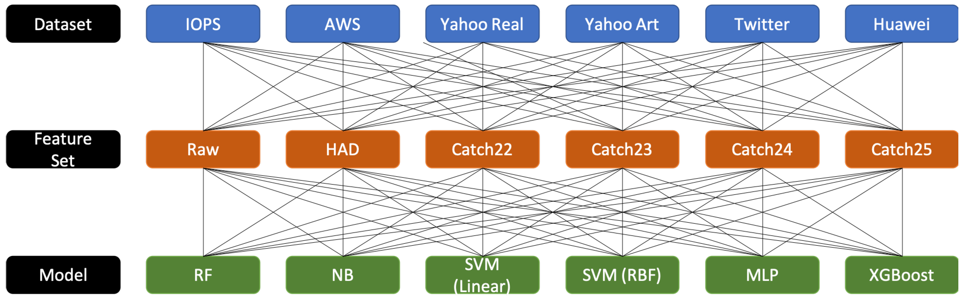
4. Experimental Design

This section provides an overview of the experimental process we used to analyse the relative effectiveness of the six different features sets for instance-based anomaly detection in cross-domain time-series. Within this study, we wish to control for model type and for domain sample. Consequently, we assess the effectiveness of each feature representation across all combinations of a number of different models and different datasets.
Following [13], we used the following set of six model types in our experiments: naïve bayes, tree-based ensembles (random forests and xgboost), feedforward neural networks, and SVM models (SVC and SVC linear). Note that the focus of this paper is on assessing the general effectiveness of different feature sets rather than on fine-tuning the performance of models. Consequently, we did not expend a large amount of time on fitting model hyper-parameters. Instead, we selected a single set of hyper-parameters for each model type and kept these consistent across the datasets. In most cases, these were the default hyper-parameters set in sklearn [40]. The following hyper-parameters were used for training each of these model types:
  • Naïve bayes: Model parameters are inferred from training data.
  • Random forest: 200 estimators, m a x _ f e a t u r e s = n _ f e a t u r e s , no max depth, two samples as minimum number of samples required to split an internal node, one as minimum number of samples in newly created leaves, with bootstrapping, using out-of-bag samples to estimate the generalization error.
  • Xgboost: gbtree booster, step size shrinkage of 0.3 , 0 Minimum loss reduction required to make a further partition on a leaf node of the tree, 6 maximum depth of a tree,
  • Multi-layer perceptron: 1 hidden layer with 100 ReLU units per layer with a single logistic unit in the output layer, adam as the solver, using L2 penalty of 0.0001, batch size of 200, constant learning rate, 0.001 step-size in updating the weights, max iterations set to 200, no early stopping, 0.9 as exponential decay rate for estimates of first moment vector, and 0.999 as exponential decay rate for estimates of second moment vector, 1 × 10 8 for numerical stability.
  • SVC: rbf kernel, regularization parameter of 1.0, scaled kernel coefficient on data set variance, and vector length.
  • SVC linear: linear kernel, and regularization parameter of 0.25.
    -
    Other SVC parameters: shrinking heuristic, no probability estimates, 1 × 10 3 tolerance for stopping criterion, 200 MB kernel cache, no class weights, no limit on number of iterations, and one-vs.-rest decision function.
We use six different datasets for analyzing the feature representations: NAB (AWS and Twitter) [41], Yahoo (Real and Artificial) [5], IOPS KPI (sometimes referred to as AIOPS in literature) (Available from: https://github.com/NetManAIOps/KPI-Anomaly-Detection (accessed on 20th May 2020), and Huawei. These datasets have time series of different time intervals and fan across different spectrum of patterns. In more detail:
  • NAB (AWS and Twitter) is a benchmark for evaluating anomaly detection algorithms in streaming, real-time applications. It is composed of over 50 labeled real-world and artificial time series. We focus on two of the real-world datasets: (i) web monitoring statistics from AWS and (ii) Twitter tweet volumes. The AWS time series are taken from different server metrics such as CPU utilization, network traffic, and disk write bytes. The Twitter dataset is the number of Twitter mentions of publicly-traded companies such as Google and IBM. The value represents the number of mentions for a given ticker symbol in every five windows.
  • Yahoo Anomaly Detection Dataset is a publicly available collection of datasets released by Yahoo for benchmarking anomaly detection algorithms. The dataset has four sets of time series: one is collected from production traffic to yahoo services, which is labelled by editors manually, whereas the others are synthesized with anomalies that are embedded artificially. We use the real data and synthesised data but not the “A3” and “A4” datasets.
  • IOPS KPI dataset is a collection of time series datasets provided by Alibaba, Tencent, Baidu, eBay, and Sogou. The dataset is from real traffic on web services and was published as part of a series of anomaly detection competitions.
  • Huawei dataset is the dataset obtained from the anomaly detection hackathon organised by Huawei (Details of the Hackathon competition are available at: https://huawei-euchallenge.bemyapp.com/ireland (accessed on 2 December 2020)). The selected time series contains different KPI values, and each datapoint is labelled as either anomaly or not anomaly.
Table 2 below provides summary statistics of the size of each dataset and the % of anomalies present in each dataset.
Algorithm 1 below provides a pseudo-code description of our experimental approach.
Algorithm 1: Structure of Experimental Design
Iot 03 00008 i001
Below, we describe the performance metrics we record and how we calculate the confidence interval for each metric, and the set of models and datasets we use.
We use F1, precision, and recall as our metrics for evaluating performance:
R = TP TP + FN
P = TP TP + FP
F 1 = 2 × P × R P + R
where P and R are precision and recall, respectively. TP, FP, and FN refer to true positive, false positive, and false negative, respectively. F1 is the main evaluation metric for our models because if we pay more attention towards precision we might miss out on some of the crucial anomalies and reduce the recall, whereas focusing on recall only may increase the number of false positives; hence, we take F1 to maintain the balance between precision and recall.
As described above for each feature set, we calculate aggregate performance metrics for F1, precision, and recall by calculating the mean value for each metric across all model types and dataset folds. In other words, given that we use five-fold cross validation, and given that we have six model types and six datasets, the mean F1 score for a feature set is calculated across a sample of (folds×model-type×dataset) 5 × 6 × 6 = 180 observations. We can calculate a confidence interval around the mean value in order to quantify the uncertainty in this mean value with respect to the unknown true mean for this feature set across the models and datasets considered using the following equation:
C I = x ¯ ± T × σ n
where x ¯ is the mean value of the observations, T is the critical value of Z-score for the respective confidence level from the T-distribution, σ is the standard deviation of the sample, and n is the number of observations in the sample. By comparing whether there is an overlap between the confidence intervals of different feature sets, we can determine whether a difference in mean performance is statistically significant at the chosen confidence level.
Figure 1 below illustrates the combinations of datasets, feature sets, and models that we used in our experiments. In the next section, we will report the results from these experiments.

5. Results

Table 3 presents for each feature set the mean F1, recall, and precision, along with the 95% confidence interval and ranges. Our initial experimental plan was that for each feature set the calculation of the mean values and confidence intervals is calculated across the set of results generated by training one instance of each of the six types of models on each of five folds per each of the six datasets. This would have meant that each mean value and confidence interval would have been calculated based on a population of 180 samples (six model types by six datasets and five folds per dataset). However, in some model/fold combinations the model did not converge, in particular the SVC and SVC Linear models failed to fit on some folds. Consequently, the observation population size per feature set was as follows: Raw:157; HAD:179; catch22:172; catch23 (catch22+SR):172; catch24 (catch22+mean+var):151; and catch25 (catch22+mean+var+SR):151.
In Table 3, we can see that the HAD feature set performs the best, followed by different variants of catch22, and the Raw feature set does not perform well at all. Examining how the inclusion of extra features into the catch22 feature set affects performance, it is interesting to note that the addition of the SR feature actually resulted in a drop in performance (both in the case of catch22 versus catch22+SR, and catch22+mean+var versus catch22+mean+var+SR). Why the inclusion of the SR feature does not help is something we will explore in future work. However, the inclusion of mean and variance features into the catch22 feature set results in improved performance (in terms of F1, recall, and precision), and, in fact, the catch24 (catch22+mean+var) has the second best performance in terms of F1 and recall and has the highest precision overall. Returning to the HAD feature set, although this feature set was the best performing in terms of F1, at the 95% confidence level there is overlap between the ranges for the mean F1 confidence interval of the HAD feature set and all the catch22-based features sets, so this good performance of the HAD feature set is not statistically different from the catch22-based feature sets at the 95% confidence interval. We also examined what would happen at a 90% confidence interval and found that there is a statistically significant difference between the HAD feature set and catch22 and catch23; however, with the addition of rolling mean and variance to the features (i.e., catch24), that margin is closed and the difference in performance is no longer statistically significant.
We also examined the mean performance by dataset and by model type. Table 4 presents the mean F1 score and confidence interval for all feature sets by model type combinations across the five folds of each dataset. Ideally, each of these mean F1 scores and confidence intervals would have been calculated across a population of 180 observations: six feature sets times six model types and times five folds. However, as noted above not all models converged on all folds, and consequently the population size for each dataset was as follows: AWS:165; Huawei: 180; IOPS:137; Twitter:165; Yahoo Artificial:170; and Yahoo Real:165.
Table 5 presents the mean F1 score and confidence interval for all feature set by dataset combinations across the six model types. Ideally, each of these mean F1 scores and confidence intervals would have been calculated across a population of 180 observations: six feature sets times six dataset times five folds. However, as noted above not all models converged on all folds, and consequently the population size for each dataset was as follows: MLP:180; Naïve Bayes:180; RF:180; SVC:163; SVC Linear:99; and Xgboost:180.
Looking at the dataset results in Table 4, the results for Yahoo Artificial are significantly better than those of the other datasets. This indicates the results on the Yahoo Artificial may be outliers that are skewing the feature set results we observed in Table 3. This consideration, together with the fact that Yahoo Artificial is a synthetic dataset, prompted us to consider removing the Yahoo Artificial results from our analysis and to examine how this would affect the relative performance of the different feature sets. Similarly, if we examine the model results in Table 5, we can observe that the best performing models are Random Forest and XGBoost and, indeed, these tree-based algorithms perform significantly better than the other models. Consequently, we also decided to remove the three weakest model types (Naïve Bayes, the SVM-based models, and multi-layer perceptron) and reexamine the results for the feature sets when these weak model results were removed. Table 6 presents the per feature set mean performance results and confidence intervals after the removal of the results for the weak models and the Yahoo Artificial feature set. The removal of these outlier values resulted in a reranking in the performance of the different feature sets: catch24 (catch22+mean+var) now performs better than HAD in terms of F1, recall, and precision. In fact, the improvement in F1 performance between the catch24 feature set and the HAD feature set is statistically significant at the 95% confidence interval, and the addition of mean and variance in catch24 provides a significant improvement in F1 score when compared to catch22 and catch23.

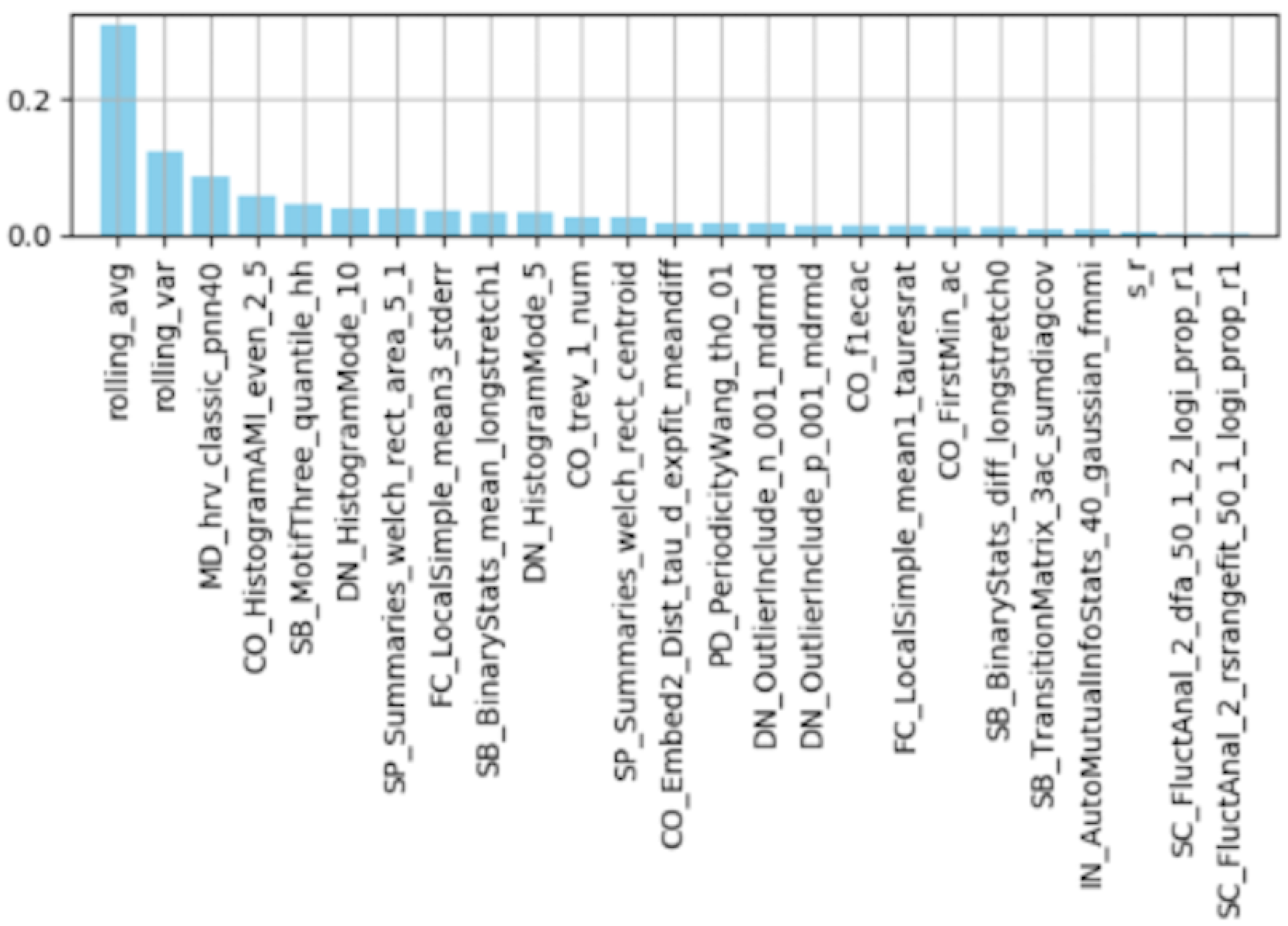
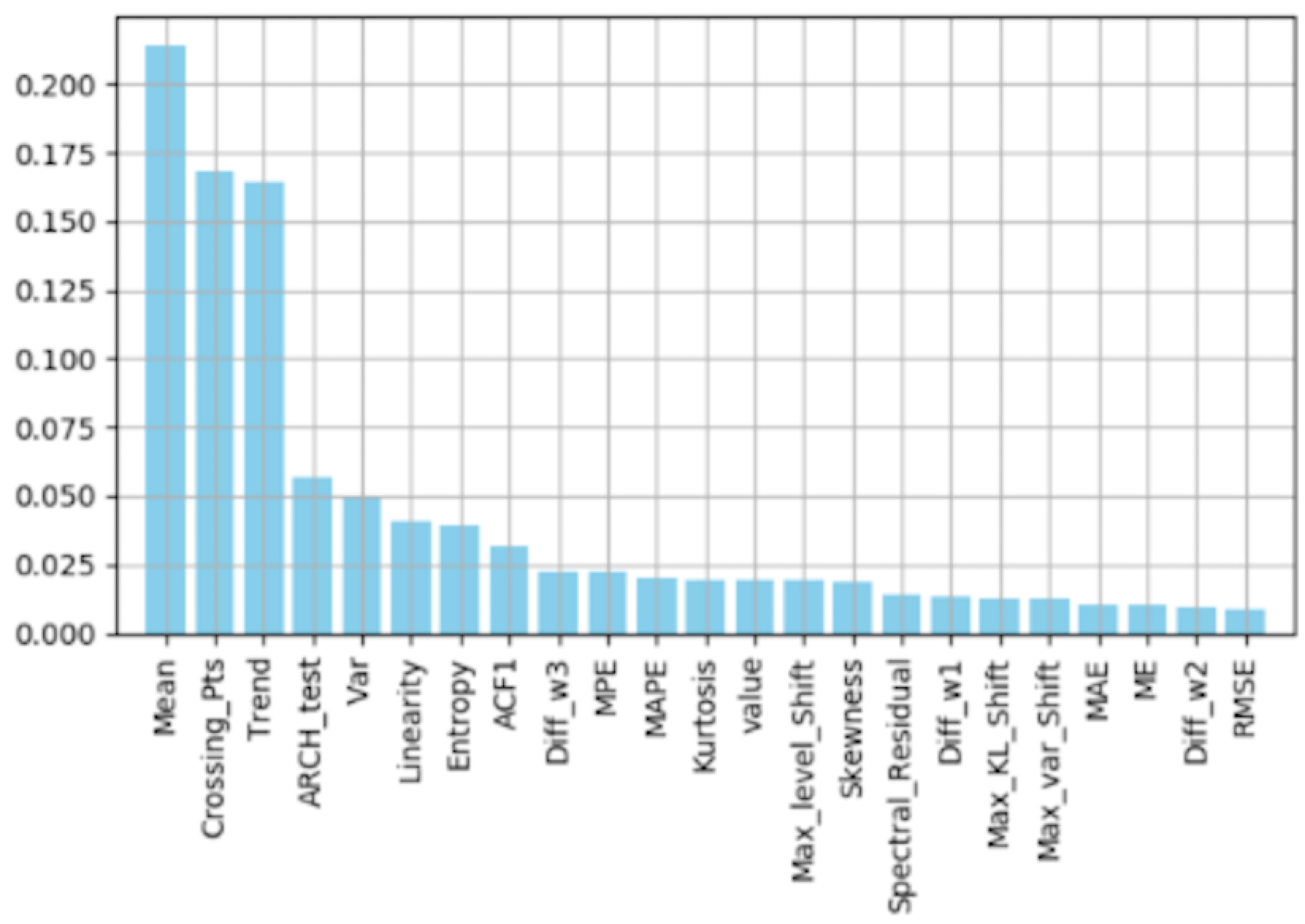
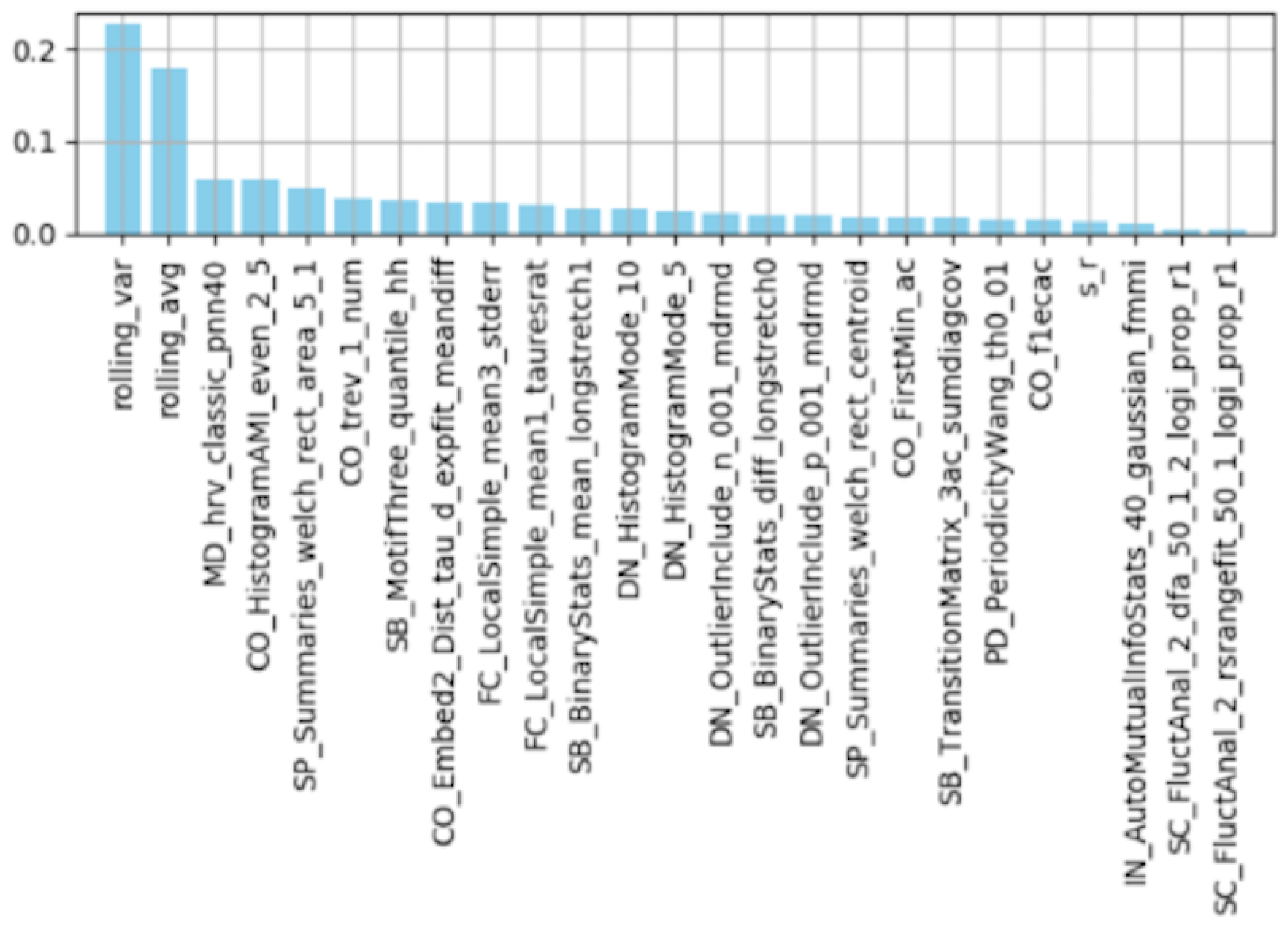
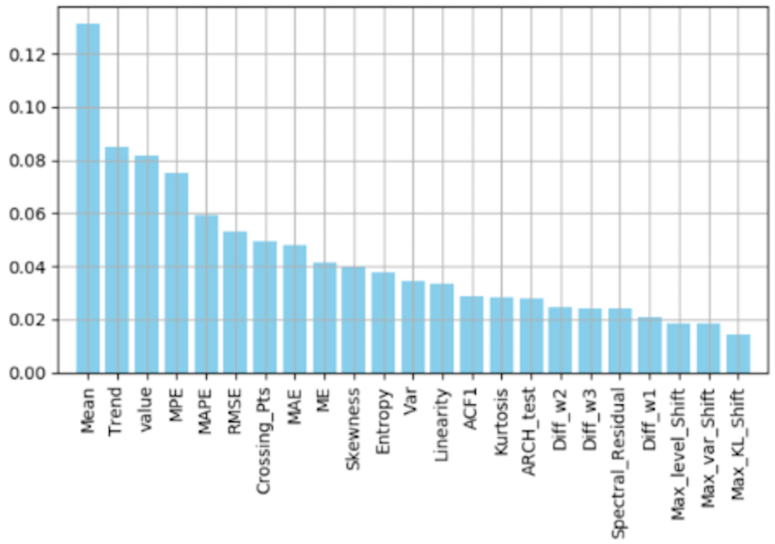
Feature Importance by Random Forest

The Random Forest model has the best overall model performance of any model type (see Table 5). The Random Forest model also has built-in feature importance, which is computed by Gini importance (mean decrease in impurity). A Random Forest is the set of decision trees (DT), and each DT is the combination of internal nodes and leaves. The selected features in the internal nodes are used to make the decision about how to divide the data into two separate sets with similar responses. The selection criterion for the internal nodes for classification tasks can be Gini impurity or information gain. Random forest measures how each feature decreases the impurity of the split. Hence, for each feature we can collect the average decreases the impurity by splitting by that feature in each tree and use this as a measure of feature importance across the ensemble of trees.
The figures below show the feature importance ranking of the features in the catch25 (we chose catch25 over catch24 because it included the largest set of features based on catch22) and the HAD feature sets for the Random Forest model when training on the Huawei and IOPS dataset (we selected these datasets as we believe they are the most representative of cross-domain anomaly detection in cloud architectures). Figure 2 and Figure 3 plot for the random forest model trained on the Huawei dataset the feature rankings from the catch25 and HAD feature sets, respectively, and Figure 4 and Figure 5 show corresponding plots for the IOPS dataset. Examining the ranking of the features, it is noticeable that features related to mean and variance are in the top three positions across all combinations of the Huawei and IOPS datasets and catch25 and HAD feature sets (note: the features termed as rolling_avg or the mean and rolling_var or var were calculated in the same way: they were computed over a moving window). More specifically, the mean feature is ranked in the top two positions in both of the datasets and feature representations, and other features such as crossing point, trend, variance, and pNN40, which are in top three positions, are indirectly extracted using mean or the variance. For example, the crossing point is the number of points crossing the mean level at the given window. These rankings of the mean and variance features align with the results of the experiments that showed that adding mean and variance improved the performance of the catch22 feature set performance.
Finally, we also noted earlier that the HAD dataset included a large number of features based on forecast errors (see Table A3, listed here for convenience: root mean squared error (RMSE), mean error (ME), mean absolute error (MAE), mean percentage error (MPE), and mean absolute percentage error (MAPE)). The inclusion of these features reflects the fact that the HAD feature set was hand-tailored towards the task of anomaly detection, and these features may be particularly useful for this task because a large forecast error may signal the presence of an anomaly. However, we also noted that the inclusion of a number of features that are likely to be correlated contrasted with the design principals of the catch22 feature set, which was specifically designed to be a feature set with minimal redundancy. Reviewing Figure 3, we can see that on the Huawei dataset these features have low importance for the model with the features ranked at 10th (MPE), 11th (MAPE), 20th (MAE), 21st (ME), and 25th or least important (RMSE). By contrast, examining Figure 5 we observe that on the IOPS dataset the random forest ranks all of these features in the top 10 most important features, at 4th (MPE), 5th (MAPE), 6th (RMSE), 8th (MAE), and 9th (ME). The fact that the ranks of these set of features changes consistently as the dataset changes indicates that these features are redundant, and likely it would be a good idea to remove some of them. Furthermore, the impact of this set of anomaly-detection-specific but redundant features is evident in the performance of the Random Forest model on these two datasets. Table 7 lists the mean F1, recall, and precision of the Random Forest model on the Huawei and IOPS datasets using the catch25 and HAD feature sets, respectively. It can be observed that on the Huawei dataset for which the model ranks these features as having low importance, the catch25 feature set outperforms the HAD feature set in precision, recall, and F1. However, for the IOPS dataset the Random Forest model returns much higher importance rankings for these forecast features, and the performance of the HAD features set on this dataset is much more competitive, resulting in higher recall and a slightly better F1 score. Overall, we take from this analysis that for some (but not all) anomaly detection datasets, including forecast error features can be useful; however, minimizing redundancy between features is likely still a useful principle.

6. Discussion

Within the field of anomaly detection for Internet of Things (IoT), a distinction can be made between (i) approaches that primarily focus on identifying abnormal data points or patterns within a data stream without reference to the structure of the network and (ii) approaches that explicitly consider the structure, type, and patterns of activations across the connections between devices in the network. In this work, we have focused on identifying anomalies within univariate time series data without reference to the structure of the cloud infrastructure or network the data was sampled from, and so our work is most closely aligned with category (i). Often, these category (i) approaches to anomaly detection are based on machine learning or statistical analysis and so do not explicitly define the structure of an anomaly [42]. Instead, in these systems feature design and feature selection are the key success factors, and it is left to the learning algorithm to induce accurate anomaly detection rules that work on the selected data representation. It is for this reason that we have focused in this work on feature set design and evaluation. For a broader perspective on this type of anomaly detection research, a well-regarded survey of the anomaly detection within this general setting (i.e., network structure agnostic) is [43], and examples of recent IoT-specific research that can be framed in this way include [44,45,46,47,48,49].
Research aligned with our second category of anomaly detection work explicitly considers the structure and/or activation patterns across a network. This type of research is sometimes referred to as graph-based or network anomaly detection, and surveys of this literature are available [43,50,51,52,53]. Often, this research uses predefined signatures or motifs of activations within a network to identify an anomaly [36]. Examples of this type of research include [54,55], and a recent example of this type of work specific to IoT is [56]. The above work on network-structure-aware anomaly detection can be understood as working on generic networks. However, the framing of IoT networks as social networks has enabled the used of social network analysis models to be applied to IoT analysis. For example, in the Social Internet of Things (SIoT) [57] framing of IoT, each node in an IoT network is understood as a social entity with social skills and, importantly, social relations with other entities (such as parental object relationship, ownership relationship, co-work object relationship, and so on). The SIoT concept has recently been expanded to the Multiple Internets of Things (MIoT), thereby allowing nodes to belong to multiple IoT networks at the same time and expanding the set of types of social relationships that a node can have with other nodes in the network [58]. The typing of relationships between nodes in a network (be it an SIoT or MIoT) expands the basis for the definition of anomalous signatures/motifs in network behavior and thereby expands the possibilities for defining network anomalies. Examples of research focused on anomaly detection in social networks, SIoT, and MIoT contexts include [42,59,60,61,62].
These two approaches to anomaly detection within IoT research can be understood as being complementary. The statistical/machine-learning-based models that omit network structure are capable of detecting unknown attacks, whereas anomaly detection methods that utilize predefined motifs or signatures across a network can struggle to identify novel anomalies but are often more accurate at detecting known anomaly types [63]. Consequently, maintaining and securing IoT and cloud infrastructure will likely involve combining both approaches.

7. Conclusions

To conclude, across the representations that we assessed we find the catch24, catch22 with the addition of variance, and mean to be the best performing feature representation. When looking at the best performing models and removing outlier datasets, we see there is a statistically significant improvement in F1 score between catch24 and both HAD and catch22, at a 95% confidence level. Looking at the importance of features reinforces that features based on mean and variance are useful for anomaly detection. For our instance-based anomaly detection task, spectral residual does not seem like a particularly useful feature. Spectral residual may be more useful to consider for sequential analysis such as recurrent architectures, because in the literature the use of this feature for anomaly detection is associated with improving the latency of the detection, which points to its use being most beneficial in sequential/recurrent time-aware models. We also found that the feature sets assessed in our experiments work best with tree-based ensemble models, although it is possible that hyperparameter tuning or additional preprocessing could improve any of the models tested. These results will feed into our future work in terms of providing a basis for selecting both the feature representations we explore and the model types we use in our experiments.

Author Contributions

Conceptualization, R.A., M.N., C.C., H.A. and J.D.K.; methodology, R.A., M.N. and J.D.K.; data curation R.A. and M.N.; experiment implementation, R.A and M.N.; analysis, R.A., M.N., and J.D.K.; writing—original draft preparation, R.A., M.N., C.C. and J.D.K.; writing—review and editing, C.C., H.A. and J.D.K.; supervision, H.A. and J.D.K.; project administration, C.C.; funding acquisition, H.A., C.C., and J.D.K. All authors have read and agreed to the published version of the manuscript.

Funding

This research was funded by Huawei Research Ireland, and by the ADAPT Centre which is funded under the SFI Research Centres Programme (Grant 13/RC/2106_P2) and is co-funded under the European Regional Development Funds.

Institutional Review Board Statement

Not applicable.

Informed Consent Statement

Not applicable.

Data Availability Statement

The Numenta Anomaly Detection Benchmark (NAB) dataset is a third party dataset accessible at: https://github.com/numenta/NAB (last accessed 13 January 2021). The Yahoo dataset is a third party dataset accessible at: https://webscope.sandbox.yahoo.com/catalog.php?datatype=s&did=70 (last accessed 13 January 2021). The IOPS KPI dataset is a third party dataset accessible from: https://github.com/NetManAIOps/KPI-Anomaly-Detection (last accessed on 13 January 2021). The Huawei dataset was obtained from the organisers of the 2020 Huawei time-series anomaly detection hackathon, the details of the hackathon competition and contact details for the organizers are available at: https://huawei-euchallenge.bemyapp.com/ireland (last accessed 13 January 2021).

Conflicts of Interest

The authors declare no conflict of interest.

Appendix A

Table A1. The catch22 feature set (based on Table 1 from [30] and reproduced here with minor formatting and wording modifications under the Creative Commons Attribution 4.0 International License (http://creativecommons.org/licenses/by/4.0/)).
FeatureDescription
DN HistogramMode 5Mode of z-scored distribution (5-bin histogram)
DN HistogramMode 10Mode of z-scored distribution (10-bin histogram)
SB BinaryStats mean longstretch1Longest period of consecutive values above the mean
DN OutlierInclude p 001 mdrmdTime intervals between successive extreme event above the mean
DN OutlierInclude n 001 mdrmdTime intervals between successive extreme events below the mean
CO f1ecacFirst 1/e crossing of autocorrelation function
CO FirstMin acFirst minimum of autocorrelation function
SP Summaries welch rect area 5 1Total power in lowest fifth of frequencies in the Fourier power spectrum
SP Summaries welch rect centroidCentroid of the Fourier power spectrum
FC LocalSimple mean3 stderrMean error from a rolling 3-sample mean
IN AutoMutualInfoStats 40 gaussian fmmiFirst minimum of the automutual information function
CO HistogramAMI even 2 5Automutual information, m = 2 , τ = 5
CO trev 1 numTime-reversibility statistic, x t + 1 x t 3 t
MD hrv classic pnn40Proportion of successive differences exceeding 0.04 σ
SB BinaryStats diff longstretch0Longest period of successive incremental decreases
SB MotifThree quantile hhShannon entropy of two successive letters in equiprobable 3 letter symbolization
FC LocalSimple mean1 tauresratChange in correlation length after iterative differencing
CO Embed2 Dist tau d expfit meandiffExponential fit to successive distances in 2-d embedding space
SC FluctAnal 2 dfa 50 1 2 logi prop r1Proportion of slower time scale fluctuations that scale with DFA ( 50 % sampling)
SC FluctAnal 2 rsrangefit 50 1 logi prop r1Proportion of slower time scale fluctuations that scale with linearly rescaled range fit
5SB TransitionMatrix 3ac sumdiagcovTrace of covariance of transition matrix between symbols in 3-letter alphabet
PD PeriodicityWang th0 01Periodicity
Table A2. The statistical feature set (based on Table 1 in [4]).
FeatureDescription
ACF1First order of autocorrelation
ACF RemainderAutocorrelation of remainder
MeanRolling mean
VarianceRolling variance
EntropySpectral entropy
LinearityStrength of linearity
TrendStrength trend
Crossing Pointnumber of crossing points
ARCHtestp value of Lagrange Multiplier (LM) test for ARCH model
CurvatureStrength of curvature computed on Trend of STL decomposition
GARCHtest.pp value of Lagrange Multiplier
Table A3. Forecasting error features (based on Table 2 in [4]).
FeatureFormulaDescription
RMSE Y i Y ^ i 2 N Root mean square error
ME Y i Y ^ i N Mean error
MAE | Y i Y ^ i | N Mean absolute error
MPE 1 N · i = 1 N Y i Y ^ i Y i Mean percentage error
MAPE 1 N · i = 1 N | Y i Y ^ i | Y i Mean absolute percentage error
Table A4. Temporal features set (based on Table 3 in [4]).
FeatureDescription
Max level shiftMax trimmed mean between two consecutive windows
Max var shiftMax variance shift between two consecutive windows
Max KL shiftMax shift in Kullback–Leibler divergence between two consecutive windows
Diff-wThe differences between the current value and the w-th previous value
LumpinessChanging variance in remainder
FlatspotsDiscretize time series value into ten equal sized interval, find maximum run length within the same bucket

References

  1. Nielsen, A. Practical Time Series Analysis: Prediction with Statistics and Machine Learning; O’Reilly Media: Sebastopol, CA, USA, 2019. [Google Scholar]
  2. Kelleher, J.D.; Tierney, B. Data Science; MIT Press: Cambridge, MA, USA, 2018. [Google Scholar]
  3. Qiu, J.; Du, Q.; Qian, C. Kpi-tsad: A time-series anomaly detector for kpi monitoring in cloud applications. Symmetry 2019, 11, 1350. [Google Scholar] [CrossRef] [Green Version]
  4. Zhang, X.; Lin, Q.; Xu, Y.; Qin, S.; Zhang, H.; Qiao, B.; Dang, Y.; Yang, X.; Cheng, Q.; Chintalapati, M.; et al. Cross-dataset Time Series Anomaly Detection for Cloud Systems. In Proceedings of the 2019 USENIX Annual Technical Conference (USENIX ATC 19), Renton, WA, USA, 10–12 July 2019; USENIX Association: Renton, WA, USA, 2019; pp. 1063–1076. [Google Scholar]
  5. Laptev, N.; Amizadeh, S.; Flint, I. Generic and scalable framework for automated time-series anomaly detection. In Proceedings of the 21th ACM SIGKDD International Conference on Knowledge Discovery and Data Mining, Sydney, Australia, 10–13 August 2015; pp. 1939–1947. [Google Scholar]
  6. Liu, D.; Zhao, Y.; Xu, H.; Sun, Y.; Pei, D.; Luo, J.; Jing, X.; Feng, M. Opprentice: Towards practical and automatic anomaly detection through machine learning. In Proceedings of the 2015 Internet Measurement Conference, Tokyo, Japan, 28–30 October 2015; pp. 211–224. [Google Scholar]
  7. Ahmad, S.; Lavin, A.; Purdy, S.; Agha, Z. Unsupervised real-time anomaly detection for streaming data. Neurocomputing 2017, 262, 134–147. [Google Scholar] [CrossRef]
  8. Terzi, D.S.; Terzi, R.; Sagiroglu, S. Big data analytics for network anomaly detection from netflow data. In Proceedings of the 2017 International Conference on Computer Science and Engineering (UBMK), Antalya, Turkey, 5–8 October 2017; pp. 592–597. [Google Scholar]
  9. Xu, H.; Chen, W.; Zhao, N.; Li, Z.; Bu, J.; Li, Z.; Liu, Y.; Zhao, Y.; Pei, D.; Feng, Y.; et al. Unsupervised anomaly detection via variational auto-encoder for seasonal KPIs in web applications. In Proceedings of the 2018 World Wide Web Conference, Lyon, France, 23–27 April 2018; pp. 187–196. [Google Scholar]
  10. Chalapathy, R.; Chawla, S. Deep learning for anomaly detection: A survey. arXiv 2019, arXiv:1901.03407. [Google Scholar]
  11. Görnitz, N.; Kloft, M.; Rieck, K.; Brefeld, U. Toward supervised anomaly detection. J. Artif. Intell. Res. 2013, 46, 235–262. [Google Scholar] [CrossRef]
  12. Kelleher, J.D. Deep Learning; MIT Press: Cambridge, MA, USA, 2019. [Google Scholar]
  13. Verner, A. LSTM Networks for Detection and Classification of Anomalies in Raw Sensor Data. Ph.D. Thesis, College of Engineering and Computing, Nova Southeastern University, Fort Lauderdale, FL, USA, 2019. [Google Scholar]
  14. Gal, Y.; Islam, R.; Ghahramani, Z. Deep bayesian active learning with image data. In Proceedings of the International Conference on Machine Learning, Sydney, Australia, 6–11 August 2017; pp. 1183–1192. [Google Scholar]
  15. Kirsch, A.; Van Amersfoort, J.; Gal, Y. Batchbald: Efficient and diverse batch acquisition for deep bayesian active learning. Adv. Neural Inf. Process. Syst. 2019, 32, 7026–7037. [Google Scholar]
  16. Hyndman, R.J.; Wang, E.; Laptev, N. Large-scale unusual time series detection. In Proceedings of the 2015 IEEE International Conference on Data Mining Workshop (ICDMW), Atlantic City, NJ, USA, 14–17 November 2015; pp. 1616–1619. [Google Scholar]
  17. Shumway, R.H.; Stoffer, D.S. Time Series Analysis and Its Applications with R Examples, 4th ed.; Springer Texts in Statistics; Springer: Berlin/Heidelberg, Germany, 2017. [Google Scholar]
  18. Chatfield, C.; Xing, H. The Analysis of Time Series: An Introduction with R, 7th ed.; Texts in Statistical Science; CRC Press: Boca Raton, FL, USA, 2019. [Google Scholar]
  19. Hyndman, R.J.; Athanasopoulos, G. Forecasting: Principles and Practice, 3rd ed.; OTexts: Melbourne, Australia, 2021. [Google Scholar]
  20. Engle, R.F. Autoregressive conditional heteroscedasticity with estimates of the variance of United Kingdom inflation. Econom. J. Econom. Soc. 1982, 50, 987–1007. [Google Scholar] [CrossRef]
  21. Bollerslev, T. Generalized autoregressive conditional heteroskedasticity. J. Econom. 1986, 31, 307–327. [Google Scholar] [CrossRef] [Green Version]
  22. Fulcher, B.D.; Little, M.A.; Jones, N.S. Highly comparative time-series analysis: The empirical structure of time series and their methods. J. R. Soc. Interface 2013, 10, 20130048. [Google Scholar] [CrossRef]
  23. Fulcher, B.D.; Jones, N.S. Highly comparative feature-based time-series classification. IEEE Trans. Knowl. Data Eng. 2014, 26, 3026–3037. [Google Scholar] [CrossRef] [Green Version]
  24. Fulcher, B.D.; Jones, N.S. hctsa: A computational framework for automated time-series phenotyping using massive feature extraction. Cell Syst. 2017, 5, 527–531. [Google Scholar] [CrossRef]
  25. O’Hara-Wild, M.; Hyndman, R.; Wang, E.; Cook, D.; Talagala, T.; Chhay, L. Feasts: Feature Extraction and Statistics for Time Series (0.2.1). 2021. Available online: https://CRAN.R-project.org/package=feasts (accessed on 17 October 2021).
  26. Hyndman, R.; Kang, Y.; Montero-Manso, P.; Talagala, T.; Wang, E.; Yang, Y.; O’Hara-Wild, M. Tsfeatures: Time Series Feature Extraction (1.0.2). 2020. Available online: https://CRAN.R-project.org/package=tsfeatures (accessed on 9 November 2021).
  27. Facebook. Kats. 2021. Available online: https://facebookresearch.github.io/Kats/ (accessed on 9 November 2021).
  28. Christ, M.; Braun, N.; Neuffer, J.; Kempa-Liehr, A.W. Time Series FeatuRe Extraction on basis of Scalable Hypothesis tests (tsfresh—A Python package). Neurocomputing 2018, 307, 72–77. [Google Scholar] [CrossRef]
  29. Barandas, M.; Folgado, D.; Fernandes, L.; Santos, S.; Abreu, M.; Bota, P.; Liu, H.; Schultz, T.; Gamboa, H. TSFEL: Time Series Feature Extraction Library. SoftwareX 2020, 11, 100456. [Google Scholar] [CrossRef]
  30. Lubba, C.H.; Sethi, S.S.; Knaute, P.; Schultz, S.R.; Fulcher, B.D.; Jones, N.S. catch22: CAnonical Time-series CHaracteristics. Data Min. Knowl. Discov. 2019, 33, 1821–1852. [Google Scholar] [CrossRef] [Green Version]
  31. Cleveland, R.; Cleveland, W.; McRae, J.E.; Terpinning, I. STL: A seasonal-trend decomposition procedure based on loess. J. Off. Stat. 1990, 6, 3–73. [Google Scholar]
  32. Henderson, T.; Fulcher, B.D. An Empirical Evaluation of Time-Series Feature Sets. arXiv 2021, arXiv:2110.10914. [Google Scholar]
  33. Ren, H.; Xu, B.; Wang, Y.; Yi, C.; Huang, C.; Kou, X.; Xing, T.; Yang, M.; Tong, J.; Zhang, Q. Time-series anomaly detection service at Microsoft. In Proceedings of the 25th ACM SIGKDD International Conference on Knowledge Discovery & Data Mining, Anchorage, AK, USA, 4–8 August 2019; pp. 3009–3017. [Google Scholar]
  34. Hou, X.; Zhang, L. Saliency detection: A spectral residual approach. In Proceedings of the 2007 IEEE Conference on Computer Vision and Pattern Recognition, Minneapolis, MN, USA, 17–22 June 2007; pp. 1–8. [Google Scholar]
  35. Vlachos, M.; Yu, P.; Castelli, V. On periodicity detection and structural periodic similarity. In Proceedings of the 2005 SIAM International Conference on Data Mining, Newport Beach, CA, USA, 21–23 April 2005; pp. 449–460. [Google Scholar]
  36. Heymann, S.; Latapy, M.; Magnien, C. Outskewer: Using skewness to spot outliers in samples and time series. In Proceedings of the 2012 IEEE/ACM International Conference on Advances in Social Networks Analysis and Mining, Istanbul, Turkey, 26–29 August 2012; pp. 527–534. [Google Scholar]
  37. Galeano, P.; Peña, D.; Tsay, R.S. Outlier detection in multivariate time series by projection pursuit. J. Am. Stat. Assoc. 2006, 101, 654–669. [Google Scholar] [CrossRef] [Green Version]
  38. Blázquez-García, A.; Conde, A.; Mori, U.; Lozano, J.A. A Review on outlier/Anomaly Detection in Time Series Data. ACM Comput. Surv. (CSUR) 2021, 54, 1–33. [Google Scholar] [CrossRef]
  39. Loperfido, N. Kurtosis-based projection pursuit for outlier detection in financial time series. Eur. J. Financ. 2020, 26, 142–164. [Google Scholar] [CrossRef]
  40. Pedregosa, F.; Varoquaux, G.; Gramfort, A.; Michel, V.; Thirion, B.; Grisel, O.; Blondel, M.; Prettenhofer, P.; Weiss, R.; Dubourg, V.; et al. Scikit-learn: Machine Learning in Python. J. Mach. Learn. Res. 2011, 12, 2825–2830. [Google Scholar]
  41. Lavin, A.; Ahmad, S. Evaluating real-time anomaly detection algorithms–the Numenta anomaly benchmark. In Proceedings of the 2015 IEEE 14th International Conference on Machine Learning and Applications (ICMLA), Miami, FL, USA, 9–11 December 2015; pp. 38–44. [Google Scholar]
  42. Cauteruccio, F.; Cinelli, L.; Corradini, E.; Terracina, G.; Ursino, D.; Virgili, L.; Savaglio, C.; Liotta, A.; Fortino, G. A framework for anomaly detection and classification in Multiple IoT scenarios. Future Gener. Comput. Syst. 2021, 114, 322–335. [Google Scholar] [CrossRef]
  43. Aggarwal, C.C.; Zhao, Y.; Philip, S.Y. Outlier detection in graph streams. In Proceedings of the 2011 IEEE 27th International Conference on Data Engineering, Hannover, Germany, 11–16 April 2011; pp. 399–409. [Google Scholar]
  44. Vanerio, J.; Casas, P. Ensemble-Learning Approaches for Network Security and Anomaly Detection. In Proceedings of the Workshop on Big Data Analytics and Machine Learning for Data Communication Networks, Los Angeles, CA, USA, 21 August 2017; Association for Computing Machinery: New York, NY, USA, 2017; pp. 1–6. [Google Scholar] [CrossRef]
  45. Nesa, N.; Ghosh, T.; Banerjee, I. Non-parametric sequence-based learning approach for outlier detection in IoT. Future Gener. Comput. Syst. 2018, 82, 412–421. [Google Scholar] [CrossRef]
  46. Pajouh, H.H.; Javidan, R.; Khayami, R.; Dehghantanha, A.; Choo, K.K.R. A Two-Layer Dimension Reduction and Two-Tier Classification Model for Anomaly-Based Intrusion Detection in IoT Backbone Networks. IEEE Trans. Emerg. Top. Comput. 2019, 7, 314–323. [Google Scholar] [CrossRef]
  47. Cauteruccio, F.; Fortino, G.; Guerrieri, A.; Liotta, A.; Mocanu, D.C.; Perra, C.; Terracina, G.; Vega, M.T. Short-long term anomaly detection in wireless sensor networks based on machine learning and multi-parameterized edit distance. Inf. Fusion 2019, 52, 13–30. [Google Scholar] [CrossRef] [Green Version]
  48. Aljawarneh, S.A.; Vangipuram, R. GARUDA: Gaussian dissimilarity measure for feature representation and anomaly detection in Internet of things. J. Supercomput. 2020, 76, 4376–4413. [Google Scholar] [CrossRef]
  49. Garg, S.; Kaur, K.; Batra, S.; Kaddoum, G.; Kumar, N.; Boukerche, A. A multi-stage anomaly detection scheme for augmenting the security in IoT-enabled applications. Future Gener. Comput. Syst. 2020, 104, 105–118. [Google Scholar] [CrossRef]
  50. Zhang, W.; Yang, Q.; Geng, Y. A survey of anomaly detection methods in networks. In Proceedings of the 2009 International Symposium on Computer Network and Multimedia Technology, Wuhan, China, 18–20 January 2009; pp. 1–3. [Google Scholar]
  51. Bhuyan, M.H.; Bhattacharyya, D.K.; Kalita, J.K. Network anomaly detection: Methods, systems and tools. IEEE Commun. Surv. Tutor. 2013, 16, 303–336. [Google Scholar] [CrossRef]
  52. Akoglu, L.; Tong, H.; Koutra, D. Graph based anomaly detection and description: A survey. Data Min. Knowl. Discov. 2015, 29, 626–688. [Google Scholar] [CrossRef] [Green Version]
  53. Ahmed, M.; Mahmood, A.N.; Hu, J. A survey of network anomaly detection techniques. J. Netw. Comput. Appl. 2016, 60, 19–31. [Google Scholar] [CrossRef]
  54. Akoglu, L.; McGlohon, M.; Faloutsos, C. Oddball: Spotting anomalies in weighted graphs. In Pacific-Asia Conference on Knowledge Discovery and Data Mining; Springer: Berlin/Heidelberg, Germany, 2010; pp. 410–421. [Google Scholar]
  55. Kovanen, L.; Karsai, M.; Kaski, K.; Kertész, J.; Saramäki, J. Temporal motifs in time-dependent networks. J. Stat. Mech. Theory Exp. 2011, 2011, P11005. [Google Scholar] [CrossRef]
  56. Li, W.; Tug, S.; Meng, W.; Wang, Y. Designing collaborative blockchained signature-based intrusion detection in IoT environments. Future Gener. Comput. Syst. 2019, 96, 481–489. [Google Scholar] [CrossRef]
  57. Atzori, L.; Iera, A.; Morabito, G.; Nitti, M. The social internet of things (siot)–when social networks meet the internet of things: Concept, architecture and network characterization. Comput. Netw. 2012, 56, 3594–3608. [Google Scholar] [CrossRef]
  58. Baldassarre, G.; Lo Giudice, P.; Musarella, L.; Ursino, D. The MIoT paradigm: Main features and an “ad-hoc” crawler. Future Gener. Comput. Syst. 2019, 92, 29–42. [Google Scholar] [CrossRef]
  59. Savage, D.; Zhang, X.; Yu, X.; Chou, P.; Wang, Q. Anomaly detection in online social networks. Soc. Netw. 2014, 39, 62–70. [Google Scholar] [CrossRef] [Green Version]
  60. Bindu, P.; Thilagam, P.S.; Ahuja, D. Discovering suspicious behavior in multilayer social networks. Comput. Hum. Behav. 2017, 73, 568–582. [Google Scholar] [CrossRef]
  61. Sharma, V.; You, I.; Kumar, R. ISMA: Intelligent Sensing Model for Anomalies Detection in Cross Platform OSNs With a Case Study on IoT. IEEE Access 2017, 5, 3284–3301. [Google Scholar] [CrossRef]
  62. Can, U.; Alatas, B. A new direction in social network analysis: Online social network analysis problems and applications. Phys. A Stat. Mech. Its Appl. 2019, 535, 122372. [Google Scholar] [CrossRef]
  63. Osanaiye, O.; Choo, K.K.R.; Dlodlo, M. Distributed denial of service (DDoS) resilience in cloud: Review and conceptual cloud DDoS mitigation framework. J. Netw. Comput. Appl. 2016, 67, 147–165. [Google Scholar] [CrossRef]
Figure 1. The combinations of datasets, feature sets, and models used in the experiments. Non-standard terminology and acronyms: catch23 is catch22+sr, catch24 is catch22+mean+variance, catch25 is catch22+sr+mean+variance, random forest (RF), Naïve Bayes (NB), multi-layer perceptron (MLP), radial basis function (RBF), and multilayer perceptron (MLP).
Iot 03 00008 g001
Figure 2. catch25 feature importance for Random Forest on Huawei dataset.
Iot 03 00008 g002
Figure 3. HAD feature importance for Random Forest on Huawei dataset.
Iot 03 00008 g003
Figure 4. catch25 feature importance for Random Forest on IOPS dataset.
Iot 03 00008 g004
Figure 5. HAD feature importance for Random Forest on IOPS dataset.
Iot 03 00008 g005
Table 1. The HAD feature set, created by adapting the feature set of [4]. Notation: N number of data points in a time series and/or set of predictions, μ T mean of values in time series T, σ T standard deviation of values in time series T, Y i the observed value at time i, Y ^ i the estimated value for time i
FeatureDescription
ACF1First order of autocorrelation
ACF RemainderAutocorrelation of remainder
MeanMean of the rolling time series window
VarianceVariance of the rolling time series window
EntropySpectral entropy (see [16])
LinearityStrength of linearity computed on the trend of STL decomposition (see [16])
TrendStrength of trend
Crossing PointNumber of crossing points (see [16])
ARCHtest.pP value of Lagrange Multiplier (LM) test for ARCH model (see [20])
CurvatureStrength of curvature computed on Trend of STL decomposition (from [16])
RMSERoot mean square error i = 1 N Y i Y ^ i 2 N
MEMean error i = 1 N Y i Y ^ i N
MAEMean absolute error i = 1 N | Y i Y ^ i | N
MPEMean percentage error 1 N · i = 1 N Y i Y ^ i Y i
MAPEMean absolute percentage error 1 N · i = 1 N | Y i Y ^ i | Y i
Max level shiftMax trimmed mean between two consecutive windows
Max var shiftMax variance shift between two consecutive windows
Max KL shiftMax shift in Kullback–Leibler divergence between two consecutive windows
Diff-wThe differences between the current value and the w-th previous value
SRFor time point i the value calculated from the SR transformed time series:
  S R i = S R i . r e a l 2 + S R i . i m a g i n a r y 2
SkewnessSkewness coefficient of the rolling time series window T = Y 1 , , Y N : S T = i = 1 N ( Y i μ T ) 3 / N σ T 3
KurtosisKurtosis coefficient of the rolling time series window T = Y 1 , , Y N : K T = i = 1 N ( Y i μ T ) 4 / N σ T 4
Table 2. Summary statistics for the datasets used in the experiment.
DatasetNumber of Points% AnomaliesNumber of Time SeriesMean Length
Yahoo Real91 K1.76%641415
Yahoo Art140 K1.76%1001415
IOPS3 M2.26%29105,985
AWS67 K4.57%1767,740
Twitter142 K0.15%10142,765
Huawei54 K4.19%69056
Table 3. For each feature set under test, the mean F1, recall, and precision, along with confidence intervals calculated to 95% and range calculated across model types and dataset fold combinations (populations sizes: 157, 179, 172, 172, 151, and 151). Bold font indicates highest score for a metric.
F1RecallPrecision
AvgConfRangeAvgConfRangeAvgConfRange
Raw (ws = 15)0.2558±0.03900.2168
0.2948
0.2263±0.03890.1873
0.2652
0.5604±0.05650.5039
0.6169
HAD0.6481±0.04640.6016
0.6945
0.6297±0.04650.5833
0.6762
0.7818±0.04600.7358
0.8278
catch220.5537±0.05280.5009
0.6066
0.5132±0.05160.4617
0.5648
0.6993±0.05410.6452
0.7534
catch230.5506±0.05250.4980
0.6031
0.509±0.05110.4579
0.5601
0.699±0.05420.6447
0.7532
catch240.5889±0.06140.5275
0.6503
0.5407±0.06080.4799
0.6015
0.7826±0.05070.7319
0.8333
catch250.5825±0.06120.5213
0.6436
0.532±0.06080.4712
0.5928
0.7812±0.05040.7308
0.8316
Table 4. Mean F1 by dataset, confidence interval calculated to 95% with population sizes 165, 180, 137, 165, 170, and 165, respectively. Bold font indicates highest average F1 score.
AverageConfidence
DataF1(Error Margin)Range
AWS0.3963±0.05490.3414
0.4512
Huawei0.5830±0.05530.5278
0.6383
IOPS0.5693±0.05130.5180
0.6206
Twitter0.3729±0.04760.3253
0.4205
Yahoo Artificial0.7724±0.03920.7333
0.8116
Yahoo Real0.4958±0.05930.4365
0.5551
Table 5. Mean F1 by model type, confidence interval calculated to 95% with population sizes 180, 180, 180, 163, 99, and 180, respectively. Bold font indicates highest average F1 score.
AverageConfidence
DataF1(Error Margin)Range
Multi-Layer
Perceptron
0.6129±0.04510.5677
0.6580
Naïve Bayes0.2386±0.02420.2144
0.2627
Random Forest0.8279±0.031100.7967
0.8590
SVC0.3259±0.046800.2791
0.3727
SVC Linear0.2233±0.07100.1524
0.2943
Xgboost0.8082±0.03220.7760
0.8404
Table 6. For each feature set under test, the mean F1, recall, and precision, along with confidence intervals, were used to calculate the 95% interval (in all cases using a population of 50 samples), and range was calculated across the results for the Random Forest and Xgboost model types and dataset fold (excluding Yahoo Artificial) combinations. Bold font indicates highest score for a metric.
F1RecallPrecision
AvgConfRangeAvgConfRangeAvgConfRange
Raw (ws = 15)0.4253±0.07000.3553
0.4954
0.3236±0.06930.2543
0.3930
0.7800±0.04450.7355
0.8245
HAD0.8675±0.02690.8406
0.8944
0.8030±0.03780.7652
0.8408
0.9556±0.01440.9412
0.9700
catch220.8434±0.03150.8119
0.8749
0.7610±0.04190.7191
0.8029
0.9598±0.01200.9478
0.9718
catch230.8360±0.03130.8047
0.8673
0.7495±0.04130.7082
0.7909
0.9587±0.01230.9464
0.9710
catch240.9167±0.01960.8971
0.9364
0.8678±0.02830.8395
0.8960
0.9766±0.00700.9696
0.9835
catch250.9161±0.01980.8964
0.9359
0.8671±0.02840.8387
0.8954
0.9760±0.00730.9687
0.9832
Table 7. Mean F1 Recall and Precision of the Random Forest model on the Huawei and IOPS datsets using the catch25 and HAD feature sets, respectively. Bold font indicates highest F1 on a dataset.
HuaweiIOPS
Prec.RecallF1Prec.RecallF1
catch250.99400.94650.96970.99080.89570.9409
HAD0.98810.87590.92870.98970.90690.9465
Publisher’s Note: MDPI stays neutral with regard to jurisdictional claims in published maps and institutional affiliations.

