Trajectory Planing for Cooperating Unmanned Aerial Vehicles in the IoT ^†

Abstract

The use of Unmanned Aerial Vehicles (UAVs) in data transport has attracted a lot of attention and applications, as a modern traffic engineering technique used in data sensing, transport, and delivery to where infrastructure is available for its interpretation. Due to UAVs’ constraints such as limited power lifetime, it has been necessary to assist them with ground sensors to gather local data, which has to be transferred to UAVs upon visiting the sensors. The management of such ground sensor communication together with a team of flying UAVs constitutes an interesting data muling problem, which still deserves to be addressed and investigated. This paper revisits the issue of traffic engineering in Internet-of-Things (IoT) settings, to assess the relevance of using UAVs for the persistent collection of sensor readings from the sensor nodes located in an environment and their delivery to base stations where further processing is performed. We propose a persistent path planning and UAV allocation model, where a team of heterogeneous UAVs coming from various base stations are used to collect data from ground sensors and deliver the collected information to their closest base stations. This problem is mathematically formalised as a real-time constrained optimisation model, and proven to be NP-hard. The paper proposes a heuristic solution to the problem and evaluates its relative efficiency through performing experiments on both artificial and real sensors networks, using various scenarios of UAVs settings.

1. Introduction

The use of UAVs has emerged as a flexible and cost-efficient alternative to traditional traffic engineering techniques that have been used in IoT settings, in order to transport sensor readings from their points of collection to their processing places. However, the joint path finding and resource allocation for a team when tasked to achieve collaborative data muling is still an issue that require further investigations. On the other hand, accurate solutions to data muling problems are still scarce, especially when considering the limited flying capacity of the battery-powered UAVs. The issues related to the efficient task allocation to a team of UAVs under stringent data collection requirements, such as real time data collection, still need to be addressed. This would benefit many task assignment models. especially when UAVs have different specifications (speeds, battery, lifetime, memory, functionalities, etc.) and only fresh and complete information need to be collected. Furthermore, persistent collection requirement needs to be addressed and this requires the data muling system to deal with outdated or premature sensor readings.

Potential applications of a such real-time data muling model include (i) city surveillance in order to evaluate risks and respond with appropriate actions by having a team of UAVs persistently visiting locations of interests in a smart city for public safety, parking spots localization [1], and pollution monitoring [2]; (ii) drought mitigation to support small scale farming in rural areas [3,4] by using a team of UAVs to collect farmland image collection and processing these images to achieve situation recognition for precision irrigation; (iii) periodic surveillance of buildings and cities’ infrastructures for structural health monitoring and maintenance; and (iv) extension of the reach of community mesh networks in rural settings for healthcare [5,6] by using a team of UAVs (such as drones) as wireless access points.

Sensors visitation under the fuel consumption constraints was addressed in [7], the visitation under the revisit deadline constraint was proposed in [8], and a path planning model has been proposed in [9,10]. Both works assumed a single moving agent (UAV), which optimally visits various targets. Ref. [11] proposes a cooperative UAVs model where many targets are visited by a team of UAVs for persistent surveillance and pursuit. In this work, the UAVs do not communicate with each other but rather rely on the information from the static underground sensors, which are optimally placed as proposed in [12]. However, all these models do not consider the persistent data delivery and heterogeneity of UAVs, which might have different fabrics and characteristics. Furthermore, neither the energy/battery consumption while the UAVs are waiting for the updated information from the terrestrial sensor network nor the penalty associated with stale information due to late visitation by the UAV to the sensor nodes have been accounted for.

While models were proposed in [13,14,15,16] for the periodic and persistent UAVs visitation of a single target from different positions, the models do not consider the path planning issues, which are as necessary as the path planning, especially for restricted environments. After deploying ground networks to assist UAV visitations [17,18,19], multiple UAV models have also been employed to visit many assisting sensors (target) [20,21]. Even if models to assist UAVs with ground sensor network have been recommended (see [18,22,23,24]), the efficient targets visitation and the assignment issue have not been addressed. However when heterogeneous UAVs have to visit multiple sensors, an UAV assignment model is required to complement path planning models.

This paper assumes a restricted and complex network, where sensors are not only connected in terms of their ability to forward data to each other, but also in terms of the possible paths UAVs may use to visit each sensor from any base station or any other sensor in a region of interest (there could be two links between two nodes). We propose a persistent and real-time path planning model together with a task allocation model, where a team of heterogeneous UAVs coming from various base stations are used to collect sensor readings from ground sensors and deliver the collected information to their closest base stations. The underlying data muling problem is (i) mathematically formalised as a real-time constrained optimisation problem, (ii) proven to be intractable, and (iii) solved using a novel heuristic solution, whose relative efficiency is proven through running experiments on both artificial and real sensor network, with various UAV settings. This paper is an extension of the work in [25]. An extension has been done by detailing the work and the proposed model has been transformed to make the model a real-time respondent. Furthermore, analysis results corresponding to added features have been provided and at this stage a real IoT network has been considered and compared with a random one.

The rest of this paper is organised as follows. The cooperative data muling model is presented in Section 2 and its algorithmic solution is provided in the same section. Simulated results are provided and discussed in Section 3 while the conclusion is drawn in Section 4.

2. The Cooperative Data Muling Model

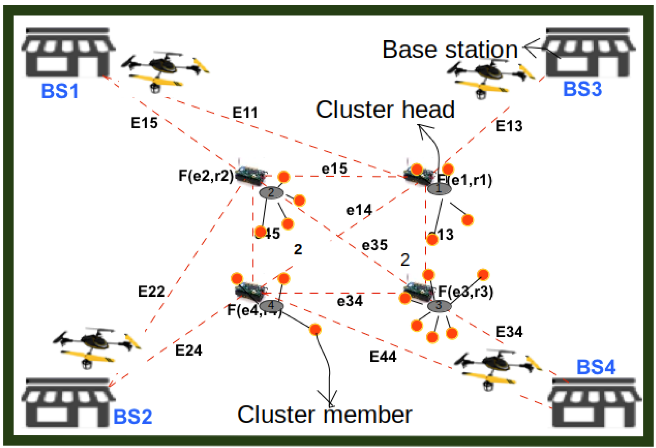
In this paper, we consider an “Internet of Things in Motion” model as shown in Figure 1. We assume that UAVs are assisted by special ground-based sensors, which locally collect data from other sensors. That is, sensors are grouped into separated clusters, each with its own sink node (the cluster head), where the information is to be collected from other sensor nodes (cluster members) and relayed to UAVs, which deliver the sensor readings to base stations. Note that only cluster heads can communicate with UAVs, and the optimal clustering scheme is not covered in this paper. Furthermore, the inner cluster communication technology is not covered here (it has been discussed in [26,27,28]).

The cooperative data muling model considered in this paper is illustrated by Figure 1. The figure reveals four base stations (B1, B2, B3 and B4) from where UAVs take off to collect data from sinks located in a region of interest and later comes back for data delivery. In this illustrative scenario, all possible collection paths that can be taken by each UAV from the base stations to access data collected by cluster heads (1, 2, 3, and 4) and deliver the collected data to the closest base stations, are represented in dotted and orange lines, whereas the continuous black lines show the communication links from sensors to their cluster heads. Here, we assume that UAVs are assisted by special nodes (cluster heads/sinks) to collect information to reduce the loss due to the UAVs capabilities (fuelling, timing, etc.). Furthermore, it is assumed that the UAV paths topology is known (this means that all possible communication paths between all sensors are known) and it is represented by small black lines in the figure. The total energy required for data collection at a node/sensor, say i, is a function $F(r_i,e_i)$ of its revisit deadline $r_i$ (the maximum amount of time required to (re)visit the node) and the energy $e_i$ required to transfer data from node i to an arriving UAV. The travel cost from a base station $B_j$ to a sink i is translated in an energy metric denoted by $E_{ij}$, and the transportation cost between two sinks i and k is also translated into an energy metric denoted by $e_{ik}$.

2.1. The Data Muling Problem

In this subsection, the problem is modelled as a constrained optimisation problem. We start by defining/denoting all cost-related terms and later we combine them to form a cost function.

2.1.1. UAVs Waiting Time on Sink Nodes

Let $t_i$ be the entire time spent by an UAV to arrive at the sink i since it took off from a base station and $r_i$ be the expected time for an UAV to arrive at the sink i. It is also referred to as revisit time at the collection point i. The sink visitation-based cost may be expressed in terms of penalties for both early and late visits on the sink nodes, the collection of information, and a risk associated with the autonomy of the UAVs. These costs are described as follows.

• Early visit penalty: an early visit penalty will be assigned to an UAV if $t_i<r_i$ to express the case where the visiting UAV arrive premature data collection. In this case, the UAV will wait for a period of time $w_i=r_i-t_i$ needed by the sink node to capture mature information from the field and transmit it to the waiting UAV;
• Late visit penalty: a late visit penalty will be applied to the UAV if $t_i>r_i$ to express the fact that the visiting UAV is late by a period of time $l_i=t_{iv}-r_i$ wasted by the UAV to arrive late to a collection point where data was ready for collection.This penalty can also be expressed using a piece-wise function;
• Data collection cost: a data collection cost will be applied to any UAV to consider the fact that the UAV has to use the energy $e_i$ to collect information from the visited node i. Note that while the costs $w_i$ and $l_i$ depend on how the terrestrial and airborne sink networks have been traffic engineered, the data collection cost $e_i$ may depend on different engineering parameters and functions, which may be bound to the communication interfaces of the equipment used by both the ground sink nodes and the UAVs and the protocol used for such communication.

For each UAV, the total cost $F(r,e_i)$ of visiting the sink i, without taking into account the travelling cost is expressed by the following equation.

$$F(r_i,e_i)=\alpha w_{i}u\left(w_i\right)+\beta l_{i}u\left(l_i\right)+\gamma e_i$$

(1)

where $u\left(w_i\right)$ and $u\left(l_i\right)$ are the values of a unit step function applied to $w_i$ and $wl$, respectively. The coefficients $\alpha$, $beta$, and $gamma$ are associated with the setting-based importance/weighting allocated to the early and late arrival penalties and the data transfer penalty, respectively.

2.1.2. The Assumed Network

We consider a hybrid sensor network (a network with multiple types of links) represented by a bi-directed graph $\mathcal{G}(\mathcal{S},\mathcal{N},\mathcal{L},\mathcal{B},\mathcal{P})$ where $\mathcal{S}$ is the set of all sensor nodes, $\mathcal{N}$ is the set of all sinks, $\mathcal{L}$ is the set of wireless communication links between the sensor nodes, $\mathcal{B}$ is the set of UAV base stations, while $\mathcal{P}$ is the set links showing the possible moves of the UAVs. Here, a move expresses one of the two following kinds of connections.

• Base station-sink: these are bidirectional UAV paths connecting sinks and base stations. The cost of moving from a base station b to a sink i is denoted $E_{bi}$ and its opposite is $E-ib$, with $E_{ib}=E_{bi}$;
• Sink-sink: these are the UAV paths connecting sinks amongst themselves and the cost to move from one sink i to j is denoted by $e_{ij}$, with $e_{ij}=e_{ji}$.

2.1.3. Initial Conditions

• Each UAV is assumed to start its journey from a base station;
• The waiting times at all sensor nodes. That is $l_i=w_j=0,\forall i,j\in N$.

Here, it is assumed that the maximum number of UAVs at each base station is equal to the degree/capacity of the base station.

2.1.4. The Data Muling Modelling

The data muling is performed in two steps

Data collection: During data collection, an UAV is to move from base station a to collect data from $k>0$ sinks labelled by a set of indices $p^{*}=[1,2,\dots ,k]$. In this case, we represent the path used for data collection by $p=[a,1,2,\dots ,k]$. The energy required for this step is expressed by the following equation.

$$C\left(p\right)=E_{a1}+\sum _{i\in p^{*}}F(r_i,e_i)+\sum _{\begin{array}{c}i,j\in P\\ j=i+1\end{array}}{e}_{ij}.$$

(2)

Data delivery: During data delivery, an  UAV may or may not pass by some already-visited sink to deliver information to the closest base station b. However, the end point of the collection path p is the starting point of the delivery path. In this case, the corresponding energy is expressed as a function $E\left(p\right)$ of the data collection path.

Therefore, the total energy $E_T\left(p\right)$ required for data collection and delivery is given by the equation

$$E_T\left(p\right)=C\left(p\right)+E\left(p\right).$$

(3)

The data muling problem consists of finding for each UAV an optimal path so that the total energy spent by all the UAVs to collect and deliver the sensor readings/data without colliding is minimized. Mathematically, we represent the set of UAVs by $U=\{1,2,3,\dots m\}$, where each UAV, u, departing from base station $a_u$ will follow path $p_u$ to collect data at locations of interest and another path (perhaps different from $pu$) to deliver the data to its closet base station. Let us consider $1_u$, the first sink to be visited by the UAV u. The data muling problem is formulated as follows.

$$MinZ=\sum _{u=1}^m\left(\sum E_{a_u{1}_u}+\sum _{i\in p_u^{*}}F(r_i,e_i)+\sum _{\begin{array}{c}i,j\in p_u^{*}\\ j=i+1\end{array}}{e}_{ij}+E\left(p_u\right)\right).$$

(4)

subject to

$$\forall v,w\in U,p_v^{*}\cap p_w^{*}=\varnothing =d\left(p_v^{*}\right)\cap d\left(p_w^{*}\right)$$

(4a)

$$\bigcup _{u\in U}{P}_u^{*}=S$$

(4b)

$$e_i,e_{ij},E\left(p\right),r,E_{a_u{1}_u}\ge 0,\forall i,j,p,a_u,1_u$$

(4c)

Here, the first constraint states that any two collection or delivery paths have no sink in common. This guarantees collision avoidance for the UAVs. On the other hand, the second constraint expresses the fact that all sinks are to be visited, and the last constraints expresses the positivity of all considered variables.

2.2. Real-Time Visitation

We consider Equation (1). In the scenarios where the variables have very strict conditions, instead of being part of the cost function, they need to be part of the problem constraints.

Table 1. Data collection scenarios.

Waiting Penalty (wi)	Late Penalty (li)	Explanation
0	0	None of the two variables is bounded
0	1	Only the late penalty is bounded
1	0	Only the waiting penalty is bounded
1	1	Both variables are bounded

shows all possible models. Here, “1” shows the case where a corresponding variable is restricted (part of the constraints) and “0” shows the other way.

The optimisation problem changes its constraints so as to become the following:

$$MinZ=\sum _{u=1}^m\left(\sum E_{a_u{1}_u}+\sum _{i\in p_u^{*}}F(r_i,e_i)+\sum _{\begin{array}{c}i,j\in p_u^{*}\\ j=i+1\end{array}}{e}_{ij}+E\left(p_u\right)\right).$$

(5)

subject to

$$\forall v,w\in U,p_v^{*}\cap p_w^{*}=\varnothing =d\left(p_v^{*}\right)\cap d\left(p_w^{*}\right)$$

(5a)

$$\bigcup _{u\in U}{P}_u^{*}=S$$

(5b)

$$0\le w_i\le W_i$$

(5c)

$$0\le l_i\le L_i$$

(5d)

$$e_i,e_{ij},E\left(p\right),r,E_{a_u{1}_u}\ge 0,foralli,j,p,a_u,1_u$$

(5e)

where $W_i$ and $L_i$ are the predetermined thresholds, which may take any non negative value.

2.3. Related Problems and Solutions

The data muling problem considered in this paper is closely related to the file recovery problem in [29] (NP-hard problem) solved by curving techniques, including those using the Parallel Unique Path (PUP) algorithm. This problem considers a case of many fragmented files, which need to be reassembled, starting from their headers, which are assumed to be known initially. The PUP algorithm is a variation of Dijkstra’s routing algorithm [30], where, starting from the headers, clusters are successively added based on their best matches.

This is done with the aim of building paths from headers having a cluster added to an existing path if and only if the link to it has the least weight. On the other hand the Vehicle Routing Problem (VRP) [31,32] consists of finding the optimal road from a depot, to be taken for delivering resources to customers and return to the depot. Exact and heuristic algorithms for its solution have been surveyed in [31]. In the survey, all stated algorithms assume a single distance matrix (the cost matrix) and hence could fail to be a good fit for our persistent visitation scenario since in our case the weighting of nodes matters and it is not a fixed value.

Furthermore, for the VRP, vehicles end their trips at the depots where they started from. This would limit the number of topologies where the data muling problem is solvable and could also impose a data muling scheme, which is not necessarily optimal. Note that in our case, we are interested in the case where the late and stale visitation are taken care of, and this depends on the dynamic position of UAVs (see the Equation (1)). Furthermore, UAVs deliver the collected information to optimal base stations (which are not necessarily their starting points).

2.4. The Data Muling Problem Intractability

To prove its intractability, we provide a polynomial reduction of one-depot VRP (which is known to be an NP-hard problem), into a special case of the data muling problem: the case where each sink’s weight is zero. The transformation consists of a two-step process, which transforms the graph $\mathcal{G}$ as follows.

• Group all base stations in in one cluster/group and consider this cluster/group as a special node for the graph, this gives the VRP’s topology ${\mathcal{G}}^{\prime }$$(\mathcal{S},\mathcal{N},\mathcal{L},$${\mathcal{B}}^{\prime }$,$\mathcal{P})$, where $\#{\mathcal{B}}^{\prime }$$=1$;
• For every link of ${\mathcal{G}}^{\prime }$, make the link weight in the new graph (found in a.) the inverse of the weight in graph ${\mathcal{G}}^{\prime }$.

This will reduce the VRP’s into the data muling problem’s solution. Clearly, the time complexity of the transformation process is polynomial, since Step a has complexity (#) and Step b has complexity (#R). The time complexity for the whole graph transformation/reduction process is therefore (#R) + (#), which is polynomial. This shows that the problem of interest in this paper is NP-hard and hence a heuristic solution is important.

2.5. The Data Muling Algorithm

In this work, we adapt Dijkstra’s algorithm in the same way it is done in [29] to solve the data muling problem. While many rounds are considered by our algorithm, we consider only the case where each node is visited only once per round. It is assumed that each UAV is capable of collecting and delivering data to a base station, where it can be recharged before going for another data collection round.

Algorithm 1 has two major steps: the first step consists of using Equation (2) to select the best node to visit for every UAV (Steps 6–7); the second step consists of adjusting the UAV’s paths by choosing the cheapest UAV for every best node (Steps 8–23). Once the visitation is done, the collection paths are captured in Cpaths and the two steps are repeated to select the nearest base station for every UAV data delivery following the delivery paths recorded by Dpaths.

Algorithm 1: Cooperative algorithm.

1 Assume a network G(N,L,B,P) as specified in Section 2.1.2;

2 $Choices\leftarrow$ all sink to be visited;

3 Initialise the path to the initial hosting base stations;

4 $done\leftarrow choices\cup B$;

5 while $choices\ne \varnothing$ do;

Proposition 1

(Polynomial termination). Algorithm 1 terminates in polynomial time when all sink nodes have been visited.

Proof. 

Note that each time a sink is included in a path of one of the UAVs, it gets excluded from the list choice (Lines 16 and 21). Since all UAV paths consist of a connected graph, whenever $choice=\varnothing$, there is at least one UAV that makes a new selection of a next sink to visit on Line 6. So, all sink are visited.

Once $choice=\varnothing$, the next destinations become the base stations and the set done = (Lines 25 and 26, consecutively). The next step is to make $\#done=\#U$ true by assigning to every UAV a base station. In this case, the statement at Line 24 is true and the set $choice=B$, which it had been updated to. This makes Algorithm 1 stop. On the other hand, the time complexity of the algorithm is clearly $\mathcal{O}({(\#U)}^2)$, which is a polynomial. Hence, the result follows. □

Remark 1.

Persistent visitation model. Since each UAV’s computed path is ended by a base station and the UAV paths form a static network, Algorithm 1 can be used repetitively to make a persistent visitation.

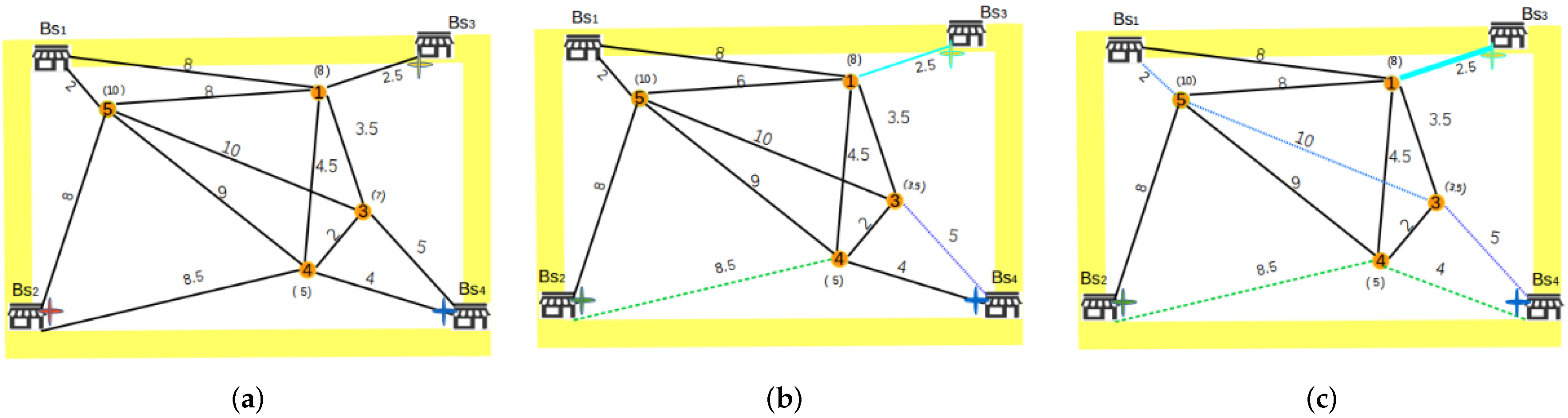
2.6. Illustration of the Algorithm

Algorithm 1 uses an example in Figure 2. We run one round of the algorithm step by step. In this example, we consider a case were each sensor node weighting is constantly zero. That is, $\alpha =\beta =0$ (see the constants in Equation (1)).

Figure 2a shows the initial conditions of the considered system. The system has four sensors, four base stations, and three UAVs positioned at all of them except for Base station Bs1. The links and sensors are weighted as discussed in Section 2. Let u2, u3, and u4 be the name of the UAVs staying at Base Stations Bs2, Bs3, and Bs4, respectively.

Figure 2b reveals how the UAVs make the choices for their first moves. The best choice is the one corresponding to the cheapest move, which is evaluated using the weight of the road to be used together with the delay at the sensor to be visited. This is why UAVs u2, u3, and u4 move to Sensors 4, 1, and 3, respectively. At this stage, only node 5 is the only node not yet visited.

Figure 2c shows the next moves up to the end of the algorithm. It shows that UAV u4 moves to Sensor 5, because it is the one corresponding to the cheapest move. On the other hand, all other UAVs do not have any other choice of sensor to visit. They then need to visit their closest base station. Once UAV u4 arrives at Node 5, it visits the closest base station, which is Bs1.

2.7. Limitation of the Proposed Model

UAVs are assumed to always have enough resources to execute the assigned tasks. It is assumed that, before departing, UAVs are fully charged (or have enough fuel) and can pass through any path which may be assigned to it. On the other hand, ground sensors are assumed to always work in perfect conditions. Furthermore, several communication models may be used to deliver data from nodes to sinks (see [26,33] for example). The task assignment model in this work has not included the communication (from nodes to sinks) cost and constrains. This has been achieved by assuming that data to be delivered at every sink would eventually be available.

3. Experimental Results

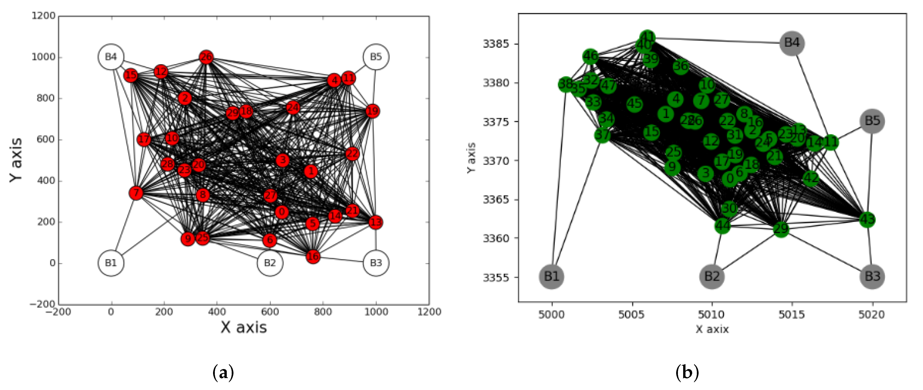
Python was used to run Algorithm 1 on two more complex networks (Figure 3a,b). The performance of the algorithm is studied and the behaviours of considered parameters are investigated. The first network (Figure 3a) consists of five base stations: B1, B2, B3, B4, and B5, as shown by bigger nodes in Figure 3a. In the figure, smaller nodes represent the sink to be visited and the links in the network show the possible paths the UAVs may take to visit the targets. 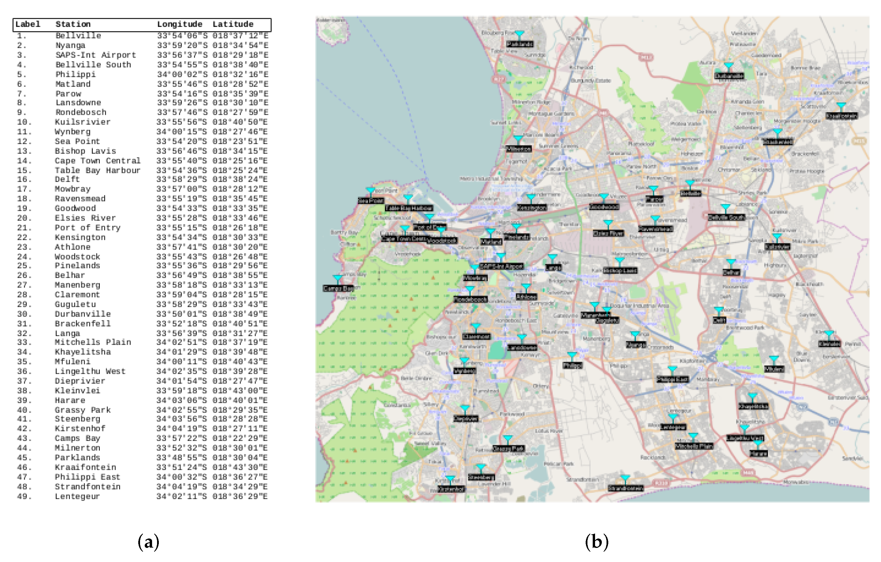Note here that the sink’s network (network without base stations) is a complete graph (each UAV is able to move from one sink to any other one in the network, but not to any base station) where nodes are randomly deployed on a 1 km${}^2$ area. On the other hand, we consider a real network (Figure 3b) consisting of the Cape Town complete network, whose nodes are police stations and their Cartesian coordinates have been extracted from GPS positions. The names corresponding to each node label are described in Appendix A (see Figure A1a,b). Note here that in these experiments the considered UAV are drones.

As shown in Figure 3a, the considered network consists of nodes randomly placed in an area of size 1 km${}^2$ and sinks are labelled in terms of the energy required to collect information from them. The coordinates of nodes in both networks are in metres and could be seen or approximated using Figure 3a,b. Positions (of sinks or base stations) consist of triples but for simplicity of plotting/viewing them, they have been projected on X-Y coordinates and hence, they are presented in the 2D Cartesian coordinate system.

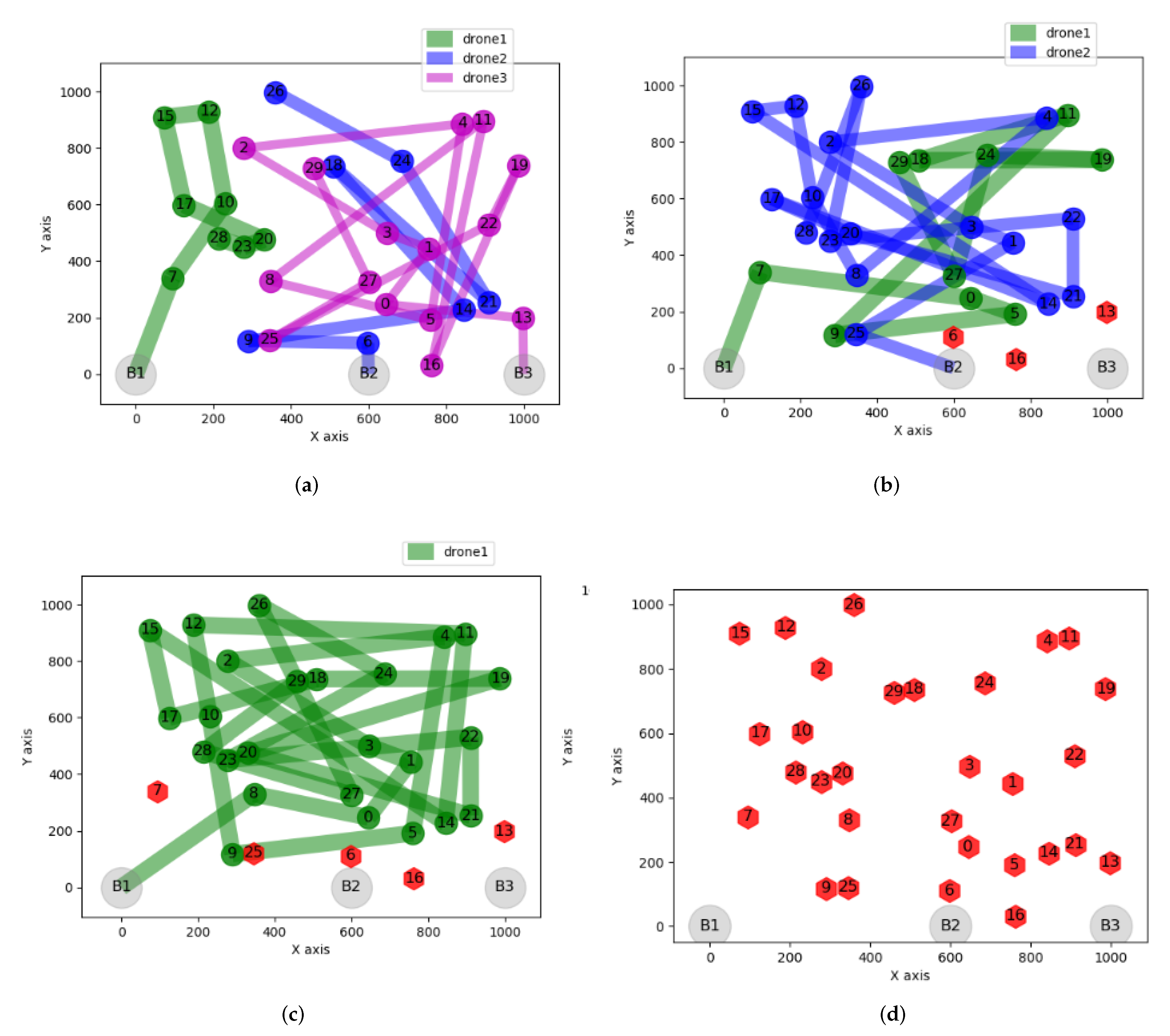
3.1. Impact of Speed Distribution on Path Planning

In two steps, we present the paths taken by UAVs using Algorithm 1.

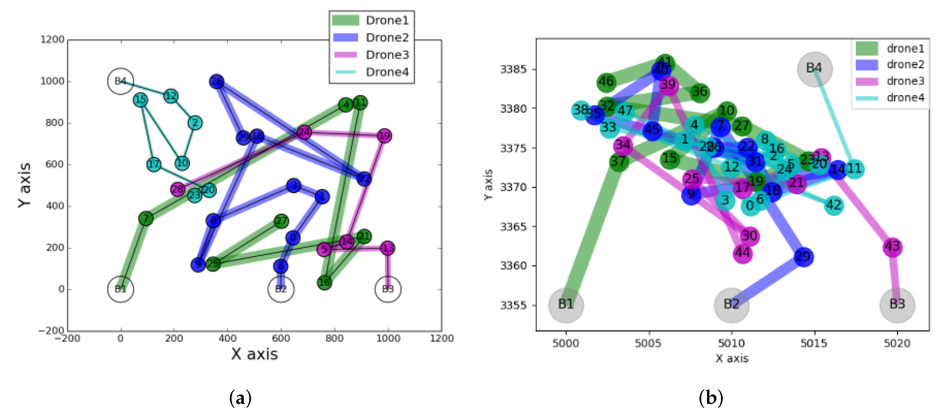
Step 1.

Data collection: it consists of visiting all sinks using the first three steps of Algorithm 1. The corresponding path for each UAV is shown in Figure 4a,b;

Step 2.

Data delivery: it consists of visiting base stations using the last step of the same algorithm. The results are shown in tables where the speed distribution of the UAVs is also presented.

The assumed cost function parameters are set to $\alpha =\beta =0.5$ and $\gamma =1$. Figure 4a,b reveals that UAVs do not visit the same number of sinks in the case of both considered networks. For example in Figure 4a, Drone1, Drone2, Drone3, and Drone4 visit sinks 7, 10, 6, and 7, respectively.

Table 2. Delivery when all speeds are the same.

(a) Delivery in the Random Network
UAV	Speed (m/min)	Source	Returning Path
Drone1	500	B1	[27, 6, B2]
Drone2	500	B2	[29, 12, B4]
Drone3	500	B3	[28, 7, B1]
Drone4	500	B4	[23, 8, B1]
(b) Delivery in the Real Network
UAV	Speed (m/min)	Source	Returning Path
Drone1	500	B1	[46, 41, B4]
Drone2	500	B2	[45, 11, B5]
Drone3	500	B3	[44, B2]
Drone4	500	B4	[47, 12, B4]

shows that when the speeds are the same for all UAVs, the delivery requires some UAVs to pass by some of the visited nodes to arrive at the base stations. This is because each sink does not need to be connected at a base station. Table 2a shows that in the case of random network, Drone3 and Drone4 deliver the collected data at the same base station (B1), and for the real network, Table 2b reveals that Drone1 and Drone4 deliver the data to B4.

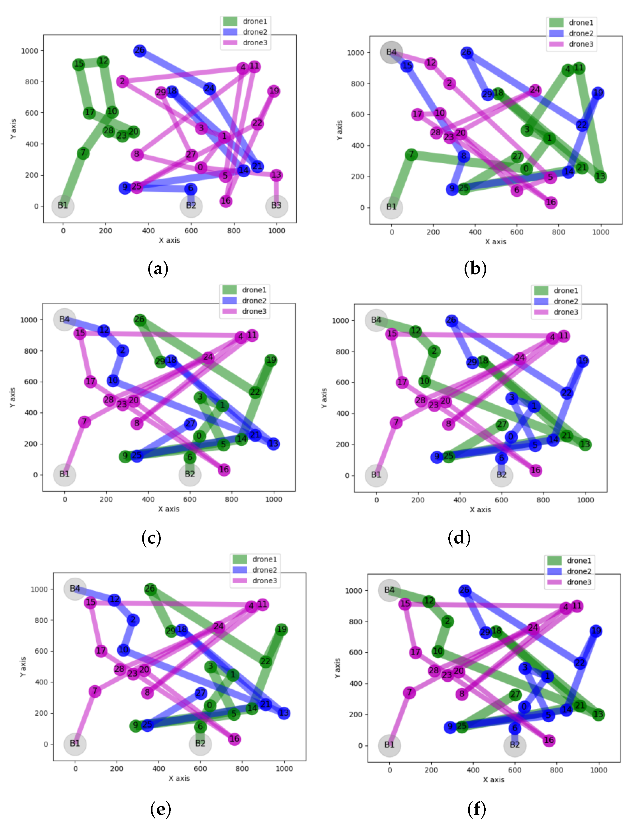
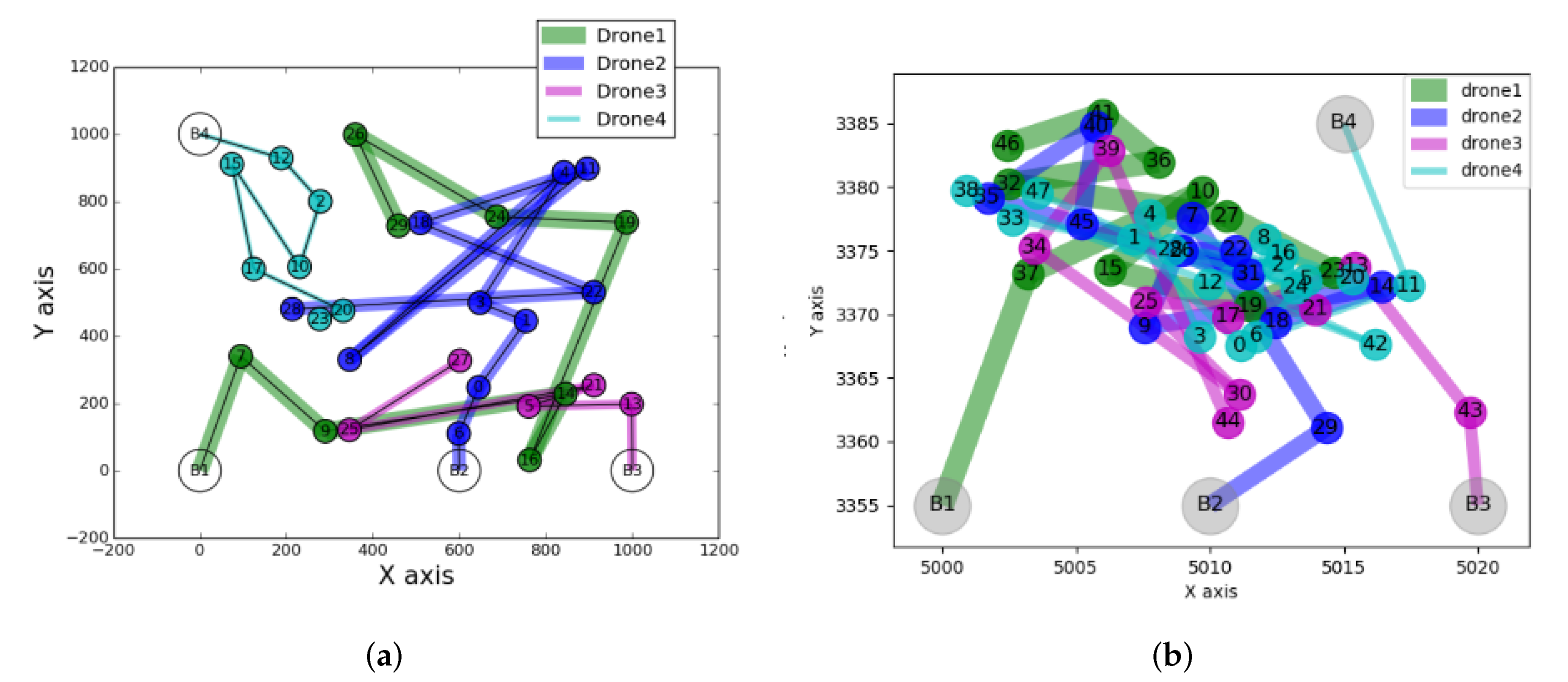
Figure 5 shows that when speeds are different, some UAVs may not change their paths but other UAVs will change their path. For example Drone4 does not change its path in both Figure 5a,b, whereas all other drones do. On the other hand, Figure 5b shows that for the real network, all drones keep their paths.

Table 3. Data delivery when all drones have a different speed.

(a) Delivery in the Random Network
UAV	Speed (m/min)	Source	Returning Path
Drone1	800	B1	[29, 12, B4]
Drone2	700	B2	[28, 7, B1]
Drone3	600	B3	[27, 6, B2]
Drone4	500	B4	[23, 8, B1]
(b) Delivery in the Real Network
UAV	Speed (m/min)	Source	Returning Path
Drone1	800	B1	[46, 41, B4]
Drone2	700	B2	[45, 11, B5]
Drone3	600	B3	[44, B2]
Drone4	500	B4	[47, 12, B4]

shows that when the speeds are different, the delivery also requires some UAVs to pass by some of the already visited nodes in order to arrive at the closest base stations. Table 3a shows that Drone2 and Drone4 deliver the collected data at the same base station (B1), and Table 3b shows that Drone1 and Drone4 deliver the collected data at the same base station (B4).

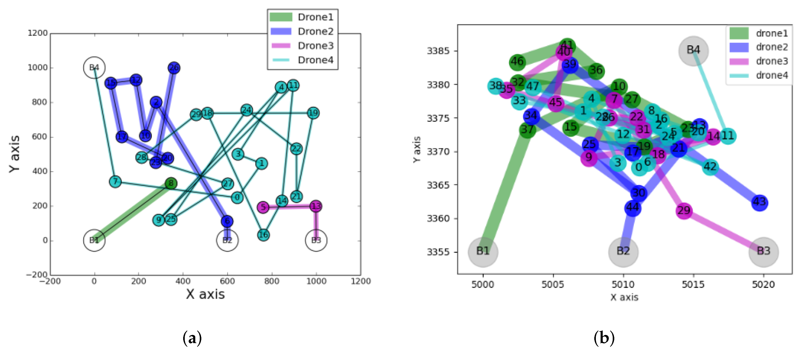
It is shown in Figure 6 that the distribution of the UAVs’ speeds have an impact on paths generation. For example Figure 6a shows that Drone1, Drone2,

Drone3, and Drone4 visit sinks 1, 9, 2, and 18, respectively. This shows a big difference due to the fact that the choice of target depends on the current and not the previous visitation costs, together with the change of speed distribution in the base stations.

Table 4. Data delivery when speed distribution changes.

(a) Delivery in the Random Network
UAV	Speed (m/min)	Source	Returning Path
Drone1	500	B1	[8, 6, B2]
Drone2	600	B2	[26, 12, B4]
Drone3	700	B3	[5, 16, B3]
Drone4	800	B4	[29, 15, B4]
(b) Delivery in the Real Network
UAV	Speed (m/min)	Source	Returning Path
Drone1	500	B1	[46, 41, B4]
Drone2	600	B2	[43, B3]
Drone3	700	B3	[45, 11, B5]
Drone4	800	B4	[47, 12, B4]

shows that when the speeds are differently distributed, the paths are changed and thus the delivery paths also change. Table 4a shows that for the random network, Drone2 and Drone4 deliver the collected data at the same base station (B4); and for the real network, Table 4b shows that Drone1 and Drone4 deliver the collected data at the same base station (B4). Since the path generation for both networks essentially behave the same, we consider (the artificial) random network for the next analysis.

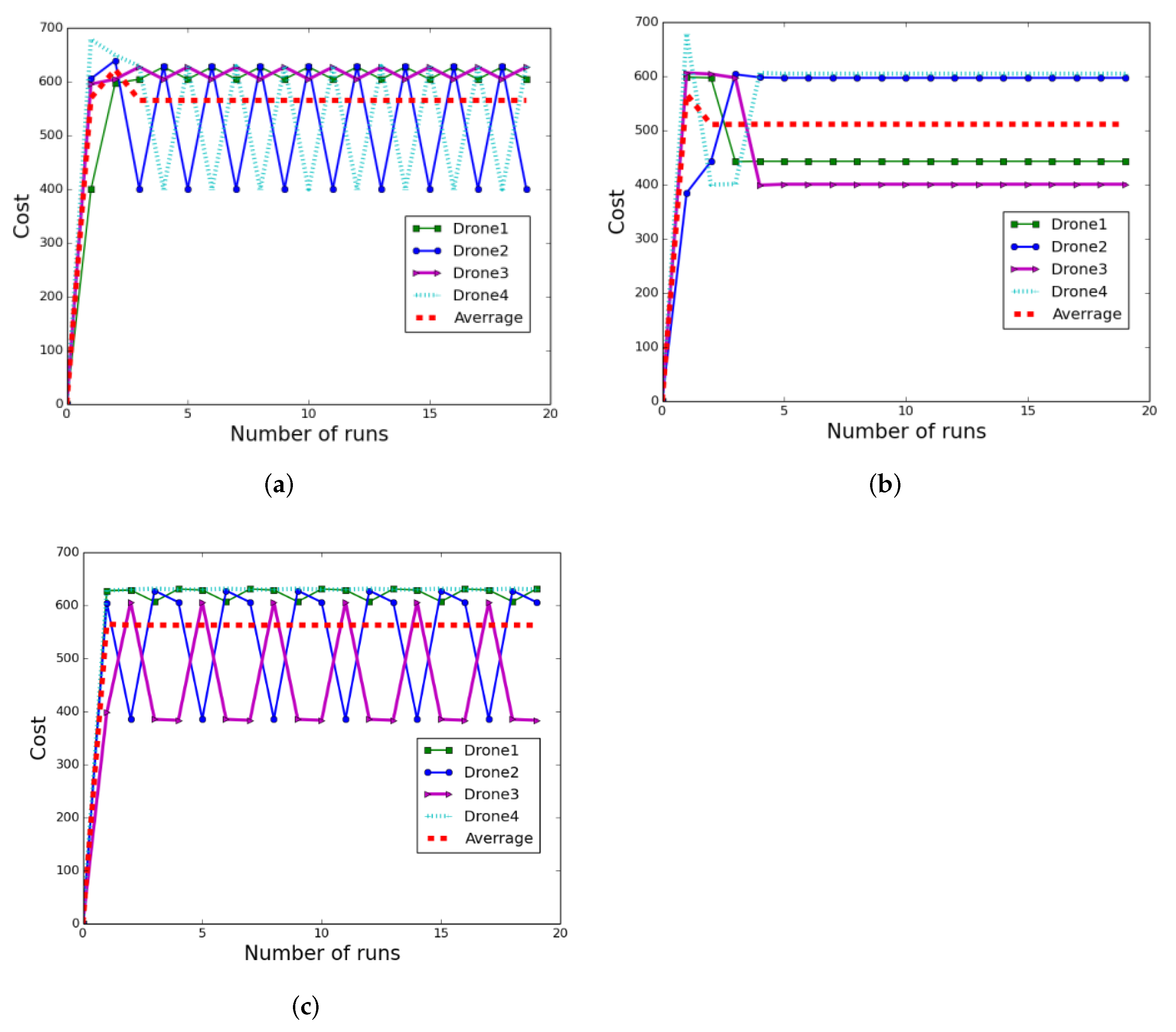
3.2. Impact of the Speed Distribution on the Cost (Total Energy)

We now study the impact of speed distribution on the cost, considering many runs of the algorithm. We perform 20 runs of Algorithm 1 in 3 cases of speed distribution, as shown by the second columns, in the tables. Figure 7a shows a case where each UAV’s speed equals 500 m/min, and on the other side Figure 7b corresponds to the case where UAVs have different speeds.

Figure 7a reveals that the cost for each drone lies in one of the few fixed values. Drone4 takes four values and all others take three and succeed each other to take the minimum and maximum values. The average cost is constantly close to 560.

Figure 7b shows that after the first four runs, all UAVs correspond to constant costs where the average cost is constantly close to 500.

Figure 7c shows that the change in speed distribution may change the average cost and also the trends of the cost function. In this case, the amended speed distribution corresponds to the one in Table 4, and shows that for each UAV, the cost changes periodically and can only take one of a few fixed values. This is why the average cost also takes one of the fixed values on a periodic basis.

3.3. Effect of Parameters Variation

In this subsection, we study the effect of four parameters on the cost variation as the number of runs varies. The four considered parameters are described as follows.

• Speed value.Keeping the speed the same for all UAVs, we aim to study the impact of its increase on the coverage cost;
• Overdue time ($\alpha$). We study the impact of overdue time on the cost. Great attention is placed on this time by incrementing the corresponding coefficient (penalty) by 0.05, for each new run;
• Delay ($\beta$). While all the other parameters are constant, we vary the parameter corresponding to the delay penalty and study how it changes the value of the coverage cost;
• Data collection rate ($\gamma$). Data collection rate is incremented by 0.05 for its value $\gamma$ = 1, of 20 runs of the algorithm.

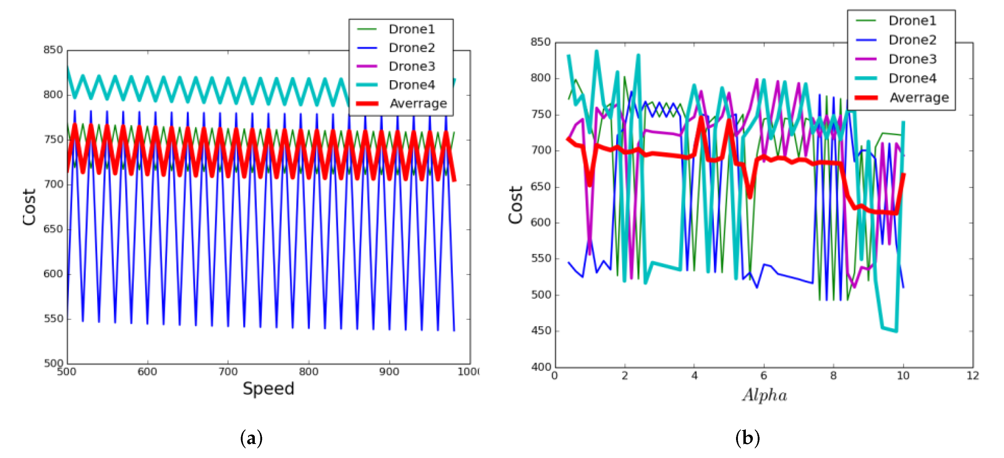
Figure 8a shows a case where the speed has been incremented 20 times for all UAVs. It shows that from the first run, each UAV periodically changes its cost between two cost values. Drone4 corresponds to the highest cost while notably Drone3 corresponds exactly to the average cost. Figure 8b shows a case where the overdue ($\alpha$) is incremented by 0.5, at each of 20 consecutive runs. The values of cost corresponding to each UAV is stochastic and the average is stochastically decreasing. We consider a case where the latency is the factor that changes in Figure 9a. The figure shows stochastic values as well but however the average cost is mostly increasing.

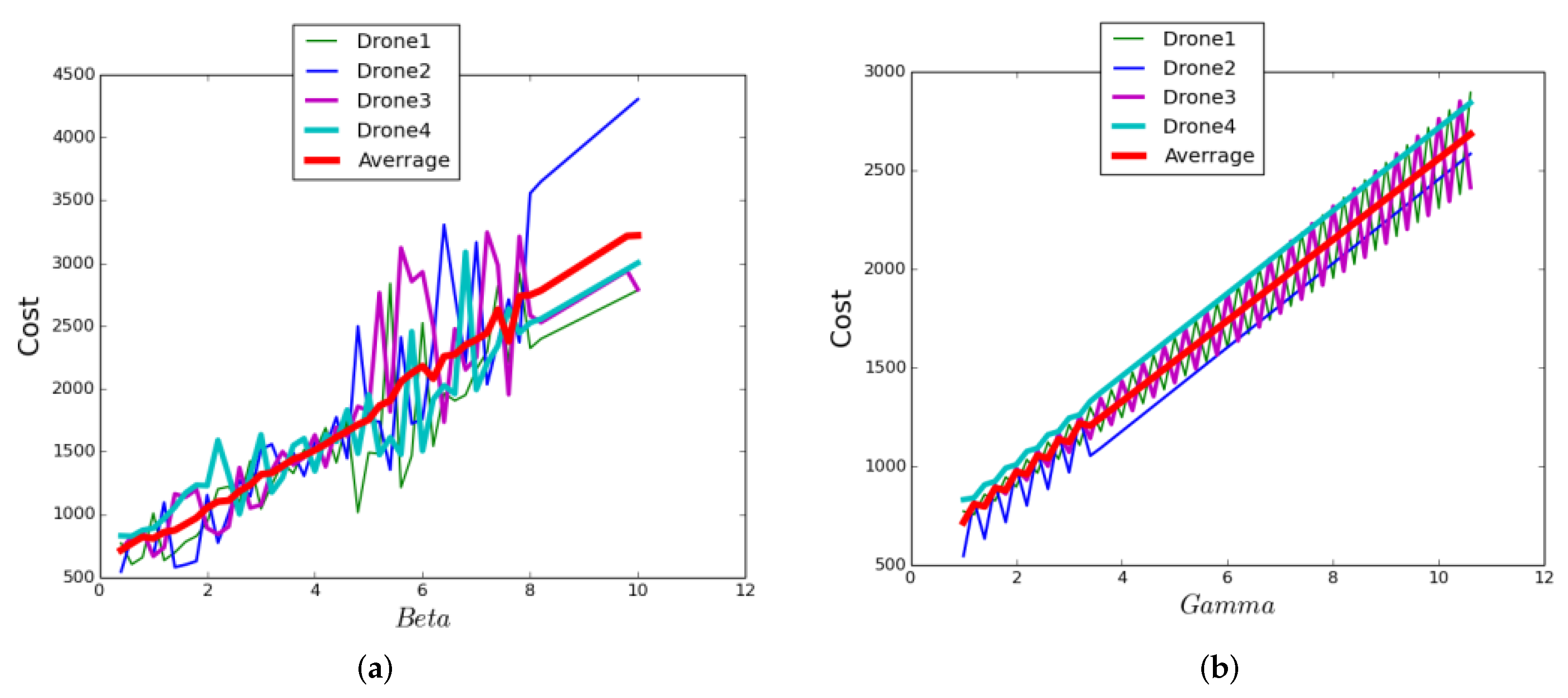
Figure 9b shows the impact of $\gamma$ on the variation of the cost over 20 runs. It shows that Drone4 mostly corresponds to the highest cost, and once $\gamma >3.8$, Drone4 and Drone2 are constantly increasing their corresponding costs, whereas the others are periodically increasing and decreasing.

3.4. Prioritisation Analysis

In this subsection, we discuss the effect of the delay and overdue time boundaries. We assume the same network as shown by Figure 3a, where the UAVs Drone1, Drone2, and Drone3 are initially positioned at Base Stations B1, B2, and B3, respectively; and all the UAVs are assumed to have the same speed v = 800 m/min.

3.4.1. Effect of Delay Constraints on Path Design

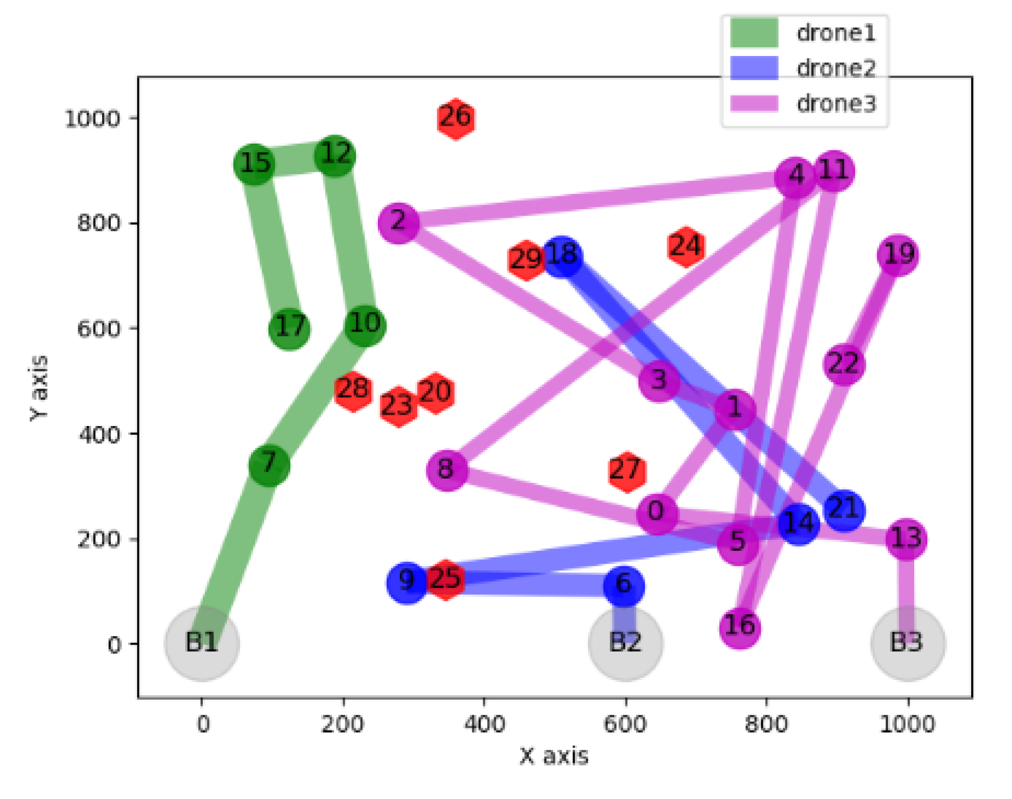
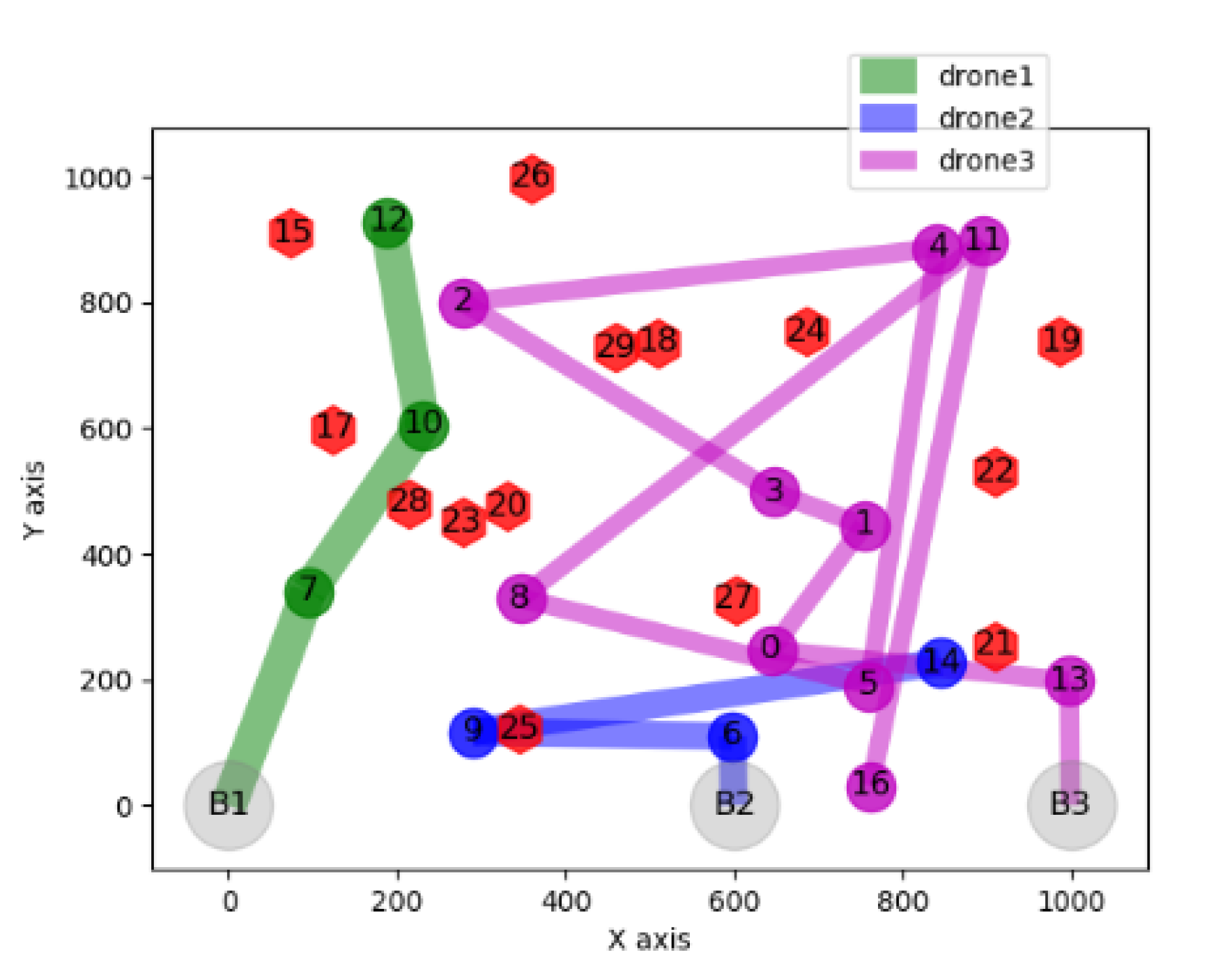
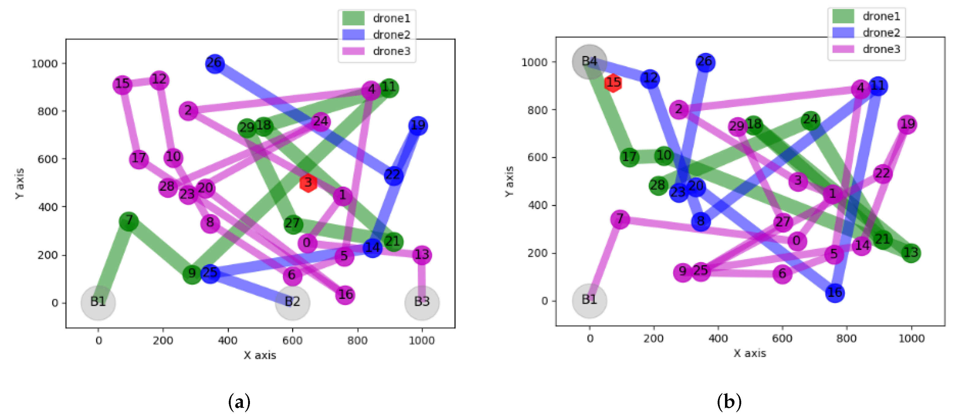
Figure 10 and

Table 5. Data delivery when UAVs may be late for no more than 30 min.

UAV	Speed (m/min)	Source	Returning Path
Drone1	800	B1	[12, B4]
Drone2	800	B2	[14, 13, B3]
Drone3	800	B3	[16, B3]

represent the case where each sensor node is visited if the arrival of a drone is late for no more than 30 min. Figure 10 shows that 14 sensor node could not be visited (see the red hexagon shaped nodes). The UAV Drone3 visited most of the nodes, whereas other UAVs could visit only three sensors each. Table 5 shows that Drone1 delivers to Base Station B4 via node 12, Drone2 to Base Station B3 via node 14 and then 13, and Drone3 to Base station B3 via node 16.

Table 6. Data delivery when UAVs may be late for no more than 60 min.

UAV	Speed (m/min)	Source	Returning Path
Drone1	800	B1	[17, B4]
Drone2	800	B2	[21, 13, B3]
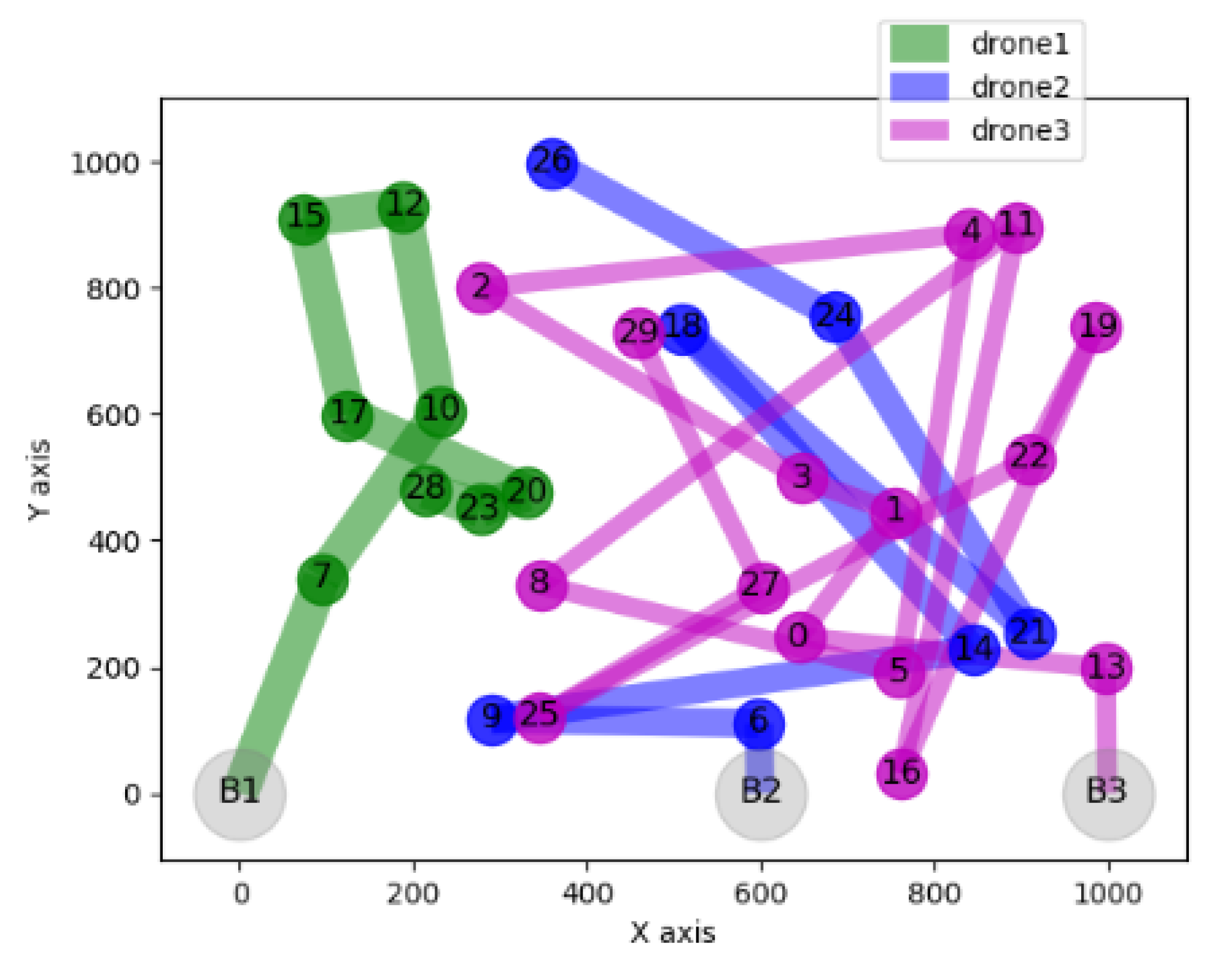
Drone3	800	B3	[22, 19, B5]

shows the data delivery paths when UAVs may be late by no more than 60 min, and Figure 11 shows the data collection path with this setting. When changing the late threshold to 60 min, Table 6 shows that the delivery paths changed, and the delivery is done as the last column of the table shows.

Compared to Figure 10, Figure 11 reveals that Drone3 does not change the path, but the other UAVs extend their path to two more sensor nodes each. This results in 10 sensor nodes to be missed, as shown by the figure.

Table 7. Data delivery when UAVs may be late for more than 60 min.

UAV	Speed (m/min)	Source	Returning Path
Drone1	800	B1	[28, 7, B1]
Drone2	800	B2	[26, 12, B4]
Drone3	800	B3	[29, 15, B4]

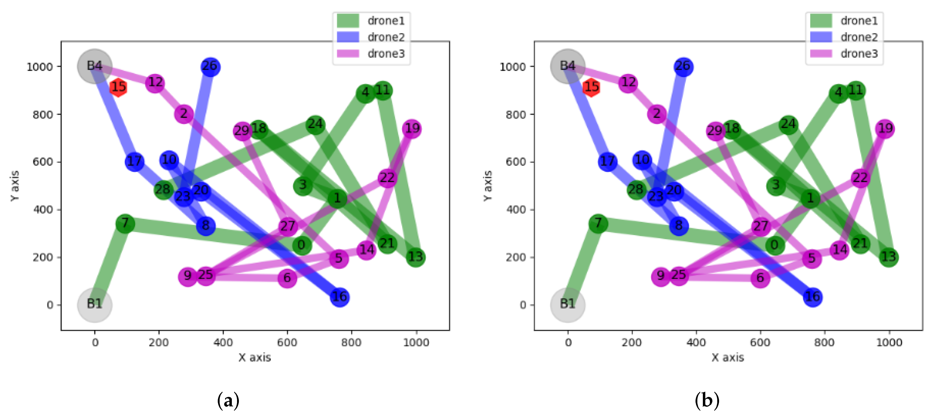
and Figure 12, respectively, show the data delivery and collection paths when UAVs may be late for a very long time.

Compared with the previous two cases, Table 7 shows that the delivery paths keep on changing. Figure 12 shows that all nodes have been visited and the path of each drone has been extended to cover more nodes.

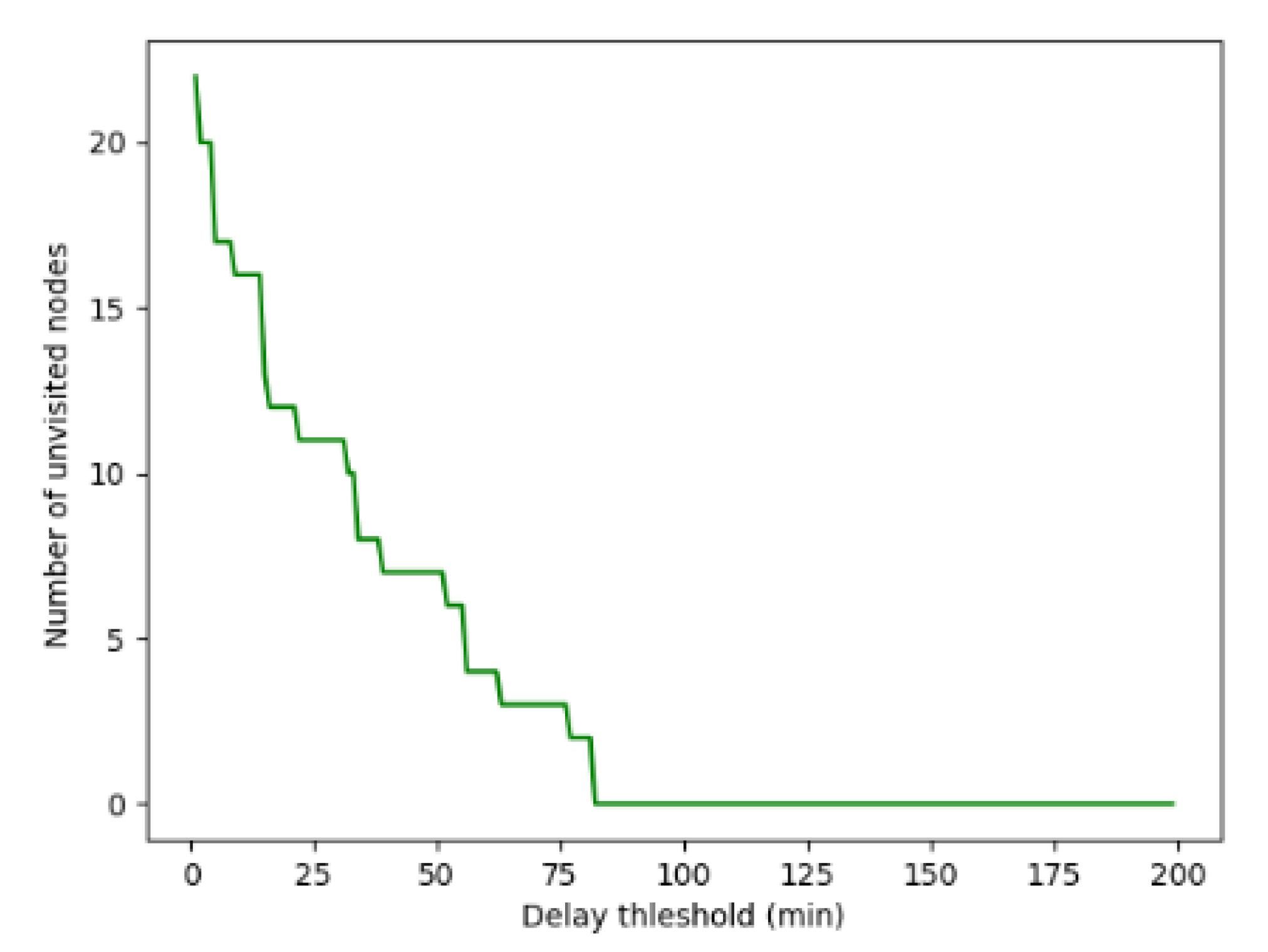
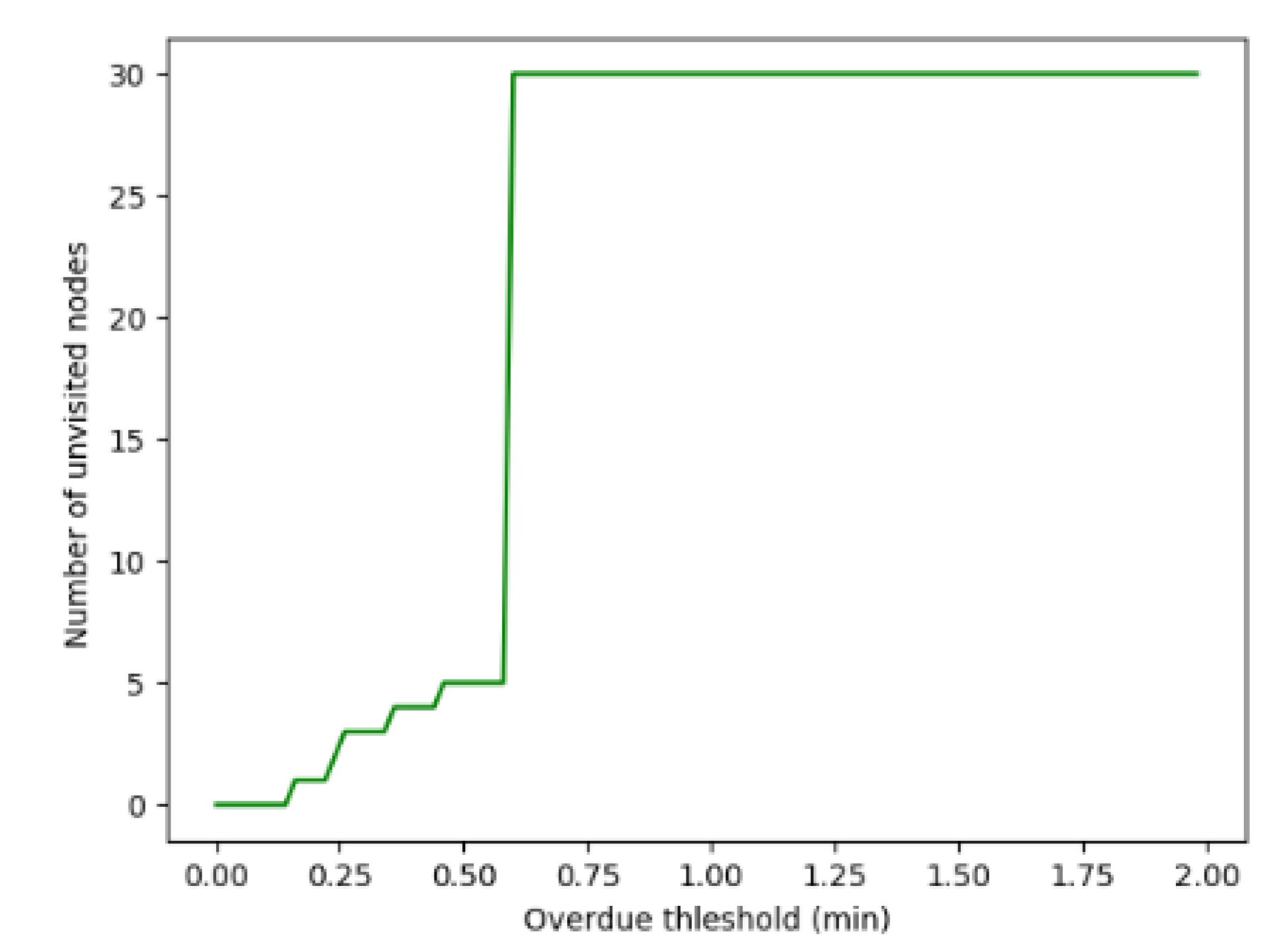
Figure 13 reveals the changes in the number of missed nodes while the late threshold evolves. The figure shows that when the delay threshold increases, the number of unvisited nodes remains constant or decreases (it never increases), until it converges to zero. This is justified by the fact that allowing a longer delay increases the chance for a node to be visited.

3.4.2. Effect of Overdue Constraints on Path Design

In this section, we study the effect of the waiting constraints. Here, sensors can only be visited after some fixed time, called the waiting threshold.

Figure 14 shows how paths corresponding to different thresholds are generated. Figure 14a considers a case where there is no waiting limitation (the waiting time is zero) and clearly all sensors are visited. When the waiting time is set to 0.3 min (18 s) in Figure 14b, three nodes are not visited and Drone 3 could not visit any sensor. Setting the waiting threshold to 0.5 min, only UAV Drone 1 could visit, and five sensors were missed (see Figure 14c). Figure 14d shows that when setting the waiting time to 0.7 min, no node could be visited. This is because there is a specific time for UAVs to arrive at each sensor, which depends on the distance and speed. If the distance is small and the UAV can arrive earlier than the waiting threshold, the visitation is impossible.

Table 8. Data delivery when the waiting threshold is small.

(a) Data Delivery When the Waiting Threshold Is 0 min
UAV	Speed (m/min)	Source	Returning Path
Drone1	800	B1	[28, 7, B1]
Drone2	800	B2	[26, 12, B4]
Drone3	800	B3	[29, 15, B4]
(b) Data Delivery When the Waiting Threshold Is 0.3 min
UAV	Speed (m/min)	Source	Returning Path
Drone1	800	B1	[29, 12, B4]
Drone2	800	B2	[28, 7, B1]
Drone3	800	B3	[B3]

and

Table 9. Data delivery when the waiting threshold is high.

(a) Data Delivery When the Waiting Threshold Is 0.5 min
UAV	Speed (m/min)	Source	Returning Path
Drone1	800	B1	[28, 7, B1]
Drone2	800	B2	[26, 12, B4]
Drone3	800	B3	[29, 15, B4]
(b) Data Delivery When the Waiting Threshold Is 0.7 min
UAV	Speed (m/min)	Source	Returning path
Drone1	800	B1	[29, 12, B4]
Drone2	800	B2	[28, 7, B1]
Drone3	800	B3	[B3]

, show deliveries corresponding to visitations shown in Figure 14. Note that if an UAV does not visit any sensor, it remains at its initial position. By changing the waiting threshold, Figure 15 shows the corresponding number of missed sensors.

Figure 15 reveals that the number of missed nodes increases as the waiting threshold increases and converges to the total number of sensors to be visited.

3.4.3. Persistent Visitation Analysis

In this subsection, we study the trend of paths when UAVs persistently visit sensors. Persistent visitation is done by resetting the initial base stations for the next visit, to the destination of the previous visitation.

Figure 16 and Figure 17 show four consecutive visitations and deliveries when the waiting threshold is set to 12 s. Figure 16a shows that only node 3 has not been visited. Figure 16b shows that a new node (node 15) has not been visited and all visitation paths change.

Figure 17a shows that paths keep on changing and non-visited nodes remain the same as the previous visitation. Note that Figure 17b is exactly the same as Figure 17a. This shows that all the following paths will be the same as Figure 17a and hence paths generation may converge to specific paths. This is a special case where the UAVs’ initial positions become the same as their optimal destination.

We now consider the constraint free visitations and study the pattern of generated paths.

Figure 18 shows the first six consecutive unconstrained visitations. The path changes, and from the third visitation the path generation becomes periodic: the third visitation is the same as the fifth, and the fourth visitation is the same as the sixth. This shows that after each visitation, the path generation remains the same. This is justified by the fact that from each base station, each UAV has a single optimal destination.

4. Conclusions and Future Work

In this paper, a model for data muling and targeting revisit costs minimization for a team of UAVs has been provided. A mathematical formulation of the model has been presented and the underlying problem has been polynomially reduced to another NP-hard problem, and hence proved to be an NP-hard problem. A heuristic solution to the problem has been provided and its performance was evaluated through simulation experiments. Simulation results have revealed different path distribution patterns under different experimental settings and the impact of these settings on path length fairness and related energy cost. Furthermore, simulations show that consecutive path generation becomes periodic after some number of visitations. Calibrating constraint parameters has shown to lead to issues of not using some UAVs, and it could reach a point where it becomes impossible to visit some or all of the nodes.

While this paper has presented the basis of a data muling model aiming at supplementing traditional traffic engineering techniques used in sink networks, several network and traffic aspects related to the proposed data muling model still need to be investigated. These include the design of efficient communication models that consider the outdoor characteristics of drone-to-sink communication, as suggested in [34]. Taking advantage of the emerging white space frequency bands as discussed in [35] to achieve drone-to-sink and drone-to-drone communication is another direction for further work. The management of ground sensors has been done in [36,37,38], but these models could be more efficient when UAVs are introduced. This will enhance many modern cyber security models such as the one proposed in [39].