Anomaly Detection and Classification in Predictive Maintenance Tasks with Zero Initial Training

Abstract

The Fourth Industrial Revolution has led to the adoption of novel technologies and methodologies in factories, making these more efficient and productive. Among the new services which are changing industry, there are those based on machine learning algorithms, which enable machines to learn from their past observations and hence possibly forecast future states. Specifically, predictive maintenance represents the opportunity to understand in advance possible machine outages due to broken parts and schedule the necessary maintenance operations. However, in real scenarios predictive maintenance struggles to be adopted due to a multitude of variables and the heavy customization it requires. In this work, we propose a novel framework for predictive maintenance, which is trained online to recognize new issues reported by the operators. Our framework, tested on different scenarios and with a varying number and several kinds of sensors, shows recall levels above 0.85, demonstrating its effectiveness and adaptability.

1. Introduction

Novel software applications and improved engineered technologies are paving the way for a radical transformation in many scenarios, including those related to the production of goods. In particular, in the industry domain this set of technologies is called Industry 4.0.

Industry 4.0 is driving an industrial revolution, encompassing a set of new technologies and novel software models which will completely transform industries. These include, for instance, Cyber Physical Systems (CPS), which provide the bridge between the software and manufacturing robots, enabling industrial machines to perform faster and better. Moreover, the adoption of machine learning models has led to a whole new set of services being offered by the industry, such as enhanced customer satisfaction management, human resources, and improved automatic control for CPS. Among the many areas that Industry 4.0 is changing, in this work we focus on predictive maintenance, which is the ability of a system to automatically predict whether some parts of a CPS are going to break before the event happens.

Maintenance costs represent between 15% and 40% of the total costs of goods production [1]. Moreover, unplanned corrective maintenance is estimated to be at least three times more expensive than a regularly scheduled one [2]. Predictive maintenance allows manufacturers to significantly reduce costs, minimizing downtimes caused by sudden breakdowns and increasing the maintenance activities that can be scheduled in advance, based on actual machine health. It also allows to substitute components just before their failure, thus making the most out of their useful lifetime.

Even though predictive maintenance has shown several benefits, particularly the increase in Overall Equipment Effectiveness (OEE) thanks to reduced stop times, its real deployment in industries is proceeding slowly, mainly due to the challenges of deploying real models in the field. One of the major obstacles to the rapid adoption of predictive maintenance models in production is the fact that the machine learning models overarching the predictive maintenance framework have to be effectively trained. This requires a dataset which collects all the sensors’ measurements, which would also contain their different readings depending on the issue that the machine is experiencing. As many variables change from machine to machine, such as standard vibrations and environmental parameters, it is challenging to have general datasets; hence, each dataset must be collected for a single machine. However, this would mean that one should know in advance all the possible issues that the machine may experience, but should also manually break it to collect the sensors’ patterns which will eventually enable the model to classify failures. In real deployments, this is clearly unfeasible, as stopping the machine to break it would increase costs of operation and slow down production, whilst it would also be difficult to foresee all the possible issues and issue levels in advance. Moreover, personnel need to be trained in advance before using novel systems such as those based on machine learning with interfaces that are different from those they are used to see. Hence, usability also takes a primary role in the adoption of Industry 4.0 technologies in industries.

To overcome these challenges, in this paper we present a novel framework which combines two different models: one is used for anomaly detection and the other for classification, which are used in cascade. Basically, the anomaly detection model is run first, collecting data about the machine in a stable state, while the classification model is run afterwards, should the anomaly detection model reports an anomaly compared to the standard state in which the machine should be. With this approach, the only data we need to bootstrap the model are those related to the machine being in the stable state, while all the other states concerning failures can be learned later by monitoring deviating states thanks to the anomaly detection model. In other words, the only input data which our model need are samples from the machine in working order. In the model we present in this paper, both the anomaly detection module and the classifier module are implemented as one-class Support Vector Machines (SVM). While in the former case the model is used to recognize anomalies—in the latter case there different one-class SVMs, each one tailored to recognize a specific issue. As soon as the anomaly detection module reports a possible new state, the raw data are fed to the classification model, which looks for patterns similar to those already seen in the past. If a match is found, then the corresponding class is output to the user, otherwise the user is asked for further details. Each time a new sample is found, the raw data are used to train a new model, with all the previous classes found, plus the new one, hence increasing the spectrum of possible issues found by the classification model. By doing this, the same model can be deployed to different industrial machines, with a different set of sensors, and the specific anomalies will be classified by the users while the model is working.

We tested our model under three different conditions to show its adaptability: first, we used a publicly available dataset; as a second scenario we built a custom prototype machine; as a third scenario we deployed our model on a real industrial machine. The results that we present in Section 5 show that our framework is able to adapt its behavior to different machines, with different numbers and types of sensors, with different machine issues and in a heterogeneous scenario.

The rest of this paper is structured as follows: Section 2 presents related work from the literature; Section 3 presents our model; Section 4 shows the datasets and scenarios we considered; Section 5 shows the different scenarios we evaluated, along with numerical results; Section 6 discusses the results obtained and the integration of this work in other scenarios; Section 7 summarizes the paper, and concludes it by also discussing future works on this topic.

2. Related Work

In recent years, industry has undergone several transformations, not only from an instrumentation point of view, but also with regard to software, human resource management, and customer relations.

Among the vast amount of work that has been carried on in the Industry 4.0 area, we focus here on contributions which focus on Condition Based Maintenance (CBM). Mainly CBM aims to reduce the costs of maintenance by performing it only when necessary, instead of doing unplanned maintenance when not needed.

Generally, each CBM operation is composed of three different phases, summarized in [3]. These steps are the Data Collection, to gather meaningful data helpful to understand the industrial machine state, the Data Management aiming at extracting useful information from the data, and finally the Decision, which defines a policy to take action related to the possible maintenance operation.

Typical CBM systems address diagnostic decisions, or prognostic decisions. While the former aims to identify a failure when it happens, the latter forecasts it, by also giving a possible time frame in which such a failure may happen. Prognostic systems are typically more complex, though they offer more valuable insights. However, they could also be combined together [4], to provide diagnostics solutions when prognostic fails. Moreover, data from the diagnostic process can be fed to the prognostic system, to strengthen its decision.

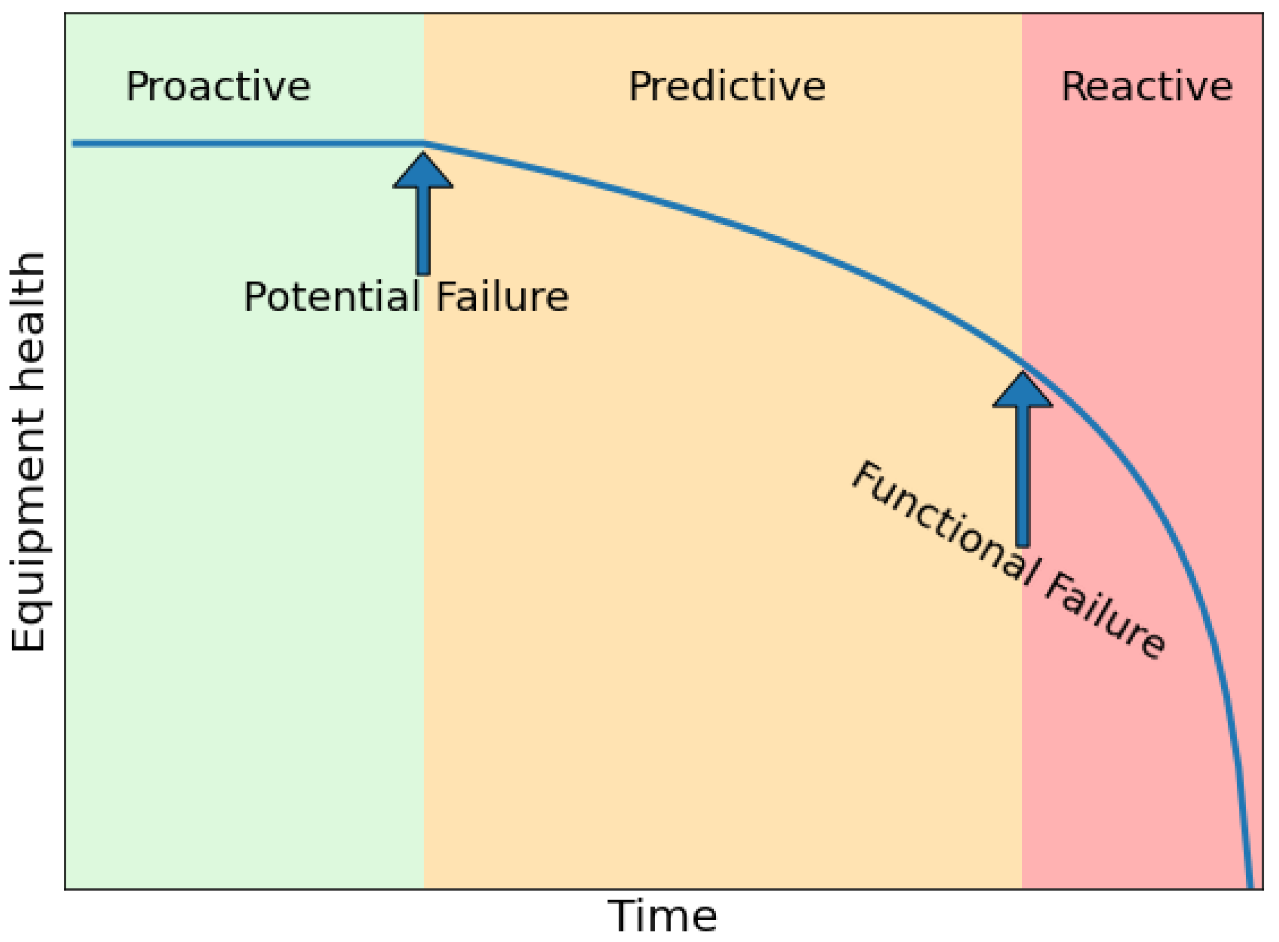
In general what any system should do is to react to potential failures in advance, before they become a functional failure for the industrial machine, typically represented by the P-F curve shown in Figure 1. Any predictive system should be able to react as soon as a potential failure is experienced, which may arise from friction, heating and other anomalies. Before such point, the maintenance would be proactive, meaning that any equipment is replaced or fixed before it actually starts to malfunction. Here, cost raises as fully functional equipment may be replaced without the need to do so. After a potential failure there is a certain time, dependent on a number of factors, in which the equipment works but the potential failure becomes more evident, until a point in which the failure becomes functional, meaning that the equipment does not work anymore, or it may break. In this scenario, predictive maintenance has not reacted fast enough, hence reactive maintenance has to take place. The time between each point and the overall lifespan of any equipment varies greatly, so in general predictive maintenance frameworks should react as fast as possible after the potential failure begins to be observed.

2.1. Data

Popular architectures for such system leverage on the cloud [5], due to the possibility of sharing data among different plants, which also helps in gathering the needed data to train appropriate models for CBM.

Data for CBM can be divided broadly in three different types. We have static data, which are those related to the kind of order the industrial machine is producing, materials in use and data about the operator following the industrial process. Then there are log data, which report the history of the machine related to maintenance operations and possible components switch. Finally there are sensor data, which are all the information coming from sensors installed in the industrial machine or in its vicinity. These can include temperature, voltage, humidity and so on, and are highly dependent on the environment and on the kind of industrial machine they are installed on.

An example of these data are provided in [6], where the authors present PRONOSTIA, a platform which aim to deliver real data for testing purposes, testifying the difficulty to gather real data for these complex scenarios.

Of course, these data are not always easy to get, hence there are different dataset which exist in the literature. For instance, NASA released datasets for two different jet2 engines, in which they simulate an engine until it reaches a state of failure [7]. They provide in total 24 variables which represent the operational characteristics of the engine, without detailing which kind of data refer to what sensor. Data are reported every 10 minutes, sampling the accelerometer values at 20 KHz for 1 second, until the industrial machine reports a failure.

Ref. [8] shows a study in which two different datasets have been used, one from a mining company and a second one from a pulp and paper company. They performed a study leveraging Principal Component Analysis, showing similarities and differences among the two datasets.

Finally there is [9], which publishes data for 100 industrial machines which span over a year. They provide telemetry data, error data, maintenance data, failure data and static data about the industrial machines.

2.2. Models

Physics based models develop systems which describe the physics characteristics of the component in terms of temperature, mechanical and chemical properties. After developing the model, which however is not an easy task, sensors reports real time values which are fed into the system. The main advantage is that this is a descriptive approach, meaning that it can be certified and explained [3]; however, it is highly challenging and it relies on the accuracy of the model.

Other models are based on the knowledge of the system, which is derived from the experience of the systems experts. Basically it transfers human knowledge to a computer understandable knowledge, such as with fuzzy logic or Bayesian networks [10]. Fuzzy logic is also the technique leveraged by [11], where the author focus specifically on gas turbine propulsion.

Finally, there are models based on big data, which use data science and machine learning applied from data collected by the industrial machines. Nowadays, it is one of the most investigated subjects in research [4], mainly because data are nowadays easier to be obtained, and they do not require deep knowledge of the system to be effective. They mainly differ on the output that the user requires from the system. There are binary classification systems, in which typically the user only wants to understand whether an issue has been identified or not [12]. Clearly multiclass systems provide more knowledge about the state of the system, but are also more complex. Regression models instead are devoted to learn the behavior of the system, in order to possibly predict its future states [13].

A further possibility which is also the one we will use in the remainder of the paper is anomaly detection. Basically the model only determines whether the system is in a standard state or not, and leaves further analysis to more specific models. The main difference among this approach and the binary classification model is that anomaly detection is semi-supervised, since it only needs to learn samples from the standard case, and it learns the non-standard ones by itself.

Some other proposals use SVMs, such as [14], where the authors build a diagnostic system for induction engines with real data gathered from engines in a standard state and during failures. A similar approach is envisioned in [15] but in a chemical scenario, and in a multiclass problem. The idea is to split the problem into several subproblems, in which they train multiple classifiers able to recognize between a class and another one. This is a solution similar to that proposed in [16] where two SVMs are combined in cascade, achieving a 94.4% of accuracy. Ref. [17] also uses an SVM but in a regression problem to estimate the Remaining Useful Life (RUL) of components.

Neural networks have been recently applied to solve CBM problems, such as in [18] and [19], where authors tackle multiclass classification problems mainly with vibration patterns, achieving over 95% of accuracy. This is also the case of [20], where the authors leveraged recurrent neural networks to develop an intelligent predictive decision support system.

Other popular algorithms used are for instance Decision Trees [21,22]. While the accuracy is over 90%, hence comparable with other techniques, author prefer Decision Trees since they can be explained and can give insights on why the failure had happened. Ref. [23] leverages instead Hidden Markov Models using the NASA dataset which we presented earlier. Each hidden state represents a different health status of the model and enables the possibility to compute the probability leading to a state of failure. The NASA dataset is also used by [24], where the authors propose a specific framework to perform prognostic condition based maintenance. Ref. [25] uses instead an Hidden semi-Markov model to generate a sequence of observations from a single state, achieving roughly 91% of accuracy in diagnostic tasks and 8.3% in prognostic tasks for the RUL of a component.

Another model often used in the literature is the Auto Regressive Integrated Moving Average (ARIMA), which is typically used to model time series behavior to forecast future trends. This is the case for the instance of [26], where the ARIMA model is used to estimate the remaining useful life of aircraft engines. Their model also employs SVM to strengthen the prediction and presents good results in this specific scenario.

2.3. Challenges

Data collection and analysis in Industry 4.0 is a complex task which encompasses a series of challenges. At first, noise can alter significantly the raw signal from the sensors, also due to environmental variables such as temperature and humidity. Thus, algorithms which analyze such data need to be robust with respect to noise, distinguishing between oscillations due to external factors and those related to possible failures. This also relates to the fact that in certain environments, it is possible that external factors alter the sensor behavior such as temperature, humidity or external vibrations.

Moreover specifically for prognostic tasks, the same failure might happen depending on various factors, making its recognition more challenging [27], as a direct causal effect may not be always evident.

However, one of the major challenges is due to the data availability itself, as data in this scenario are not easy to gather, since that would mean to physically break the industrial machine in all the possible ways in which it could lead to a failure, which is clearly unfeasible due to raised operational costs and also to the fact that operators should know in advance all the possible issues which the industrial machine may experience. Hence algorithms should work with few data available, and learn issues online rather than being trained once at deployment time. This allows for rapid deployment of the predictive maintenance algorithms which learn as the available dataset grows. Moreover it is also challenging to design systems which can adapt to a number of different scenarios, with heterogeneous sensors and with a varying set of issues to be recognized. The system we propose in this paper addresses these challenges in the following way:

• Data Collection: our system does not need any input data when installed in a new industrial machine, and it is able to learn as the machine operates. The only mandatory operation is that when installed, the machine should be in correct working order, i.e., it should not have any issue. This can be easily done for instance when ordinary and extraordinary maintenance operations are planned: upon completing the maintenance, the system may be run and learns what is the behavior of the machine in a correct working operation.
• Causality: our system does not recognize specific causality but leaves to the operator the possibility to describe the anomaly which the system experienced. In other words, we do not look to understand what specific component is responsible for the issue, but the system presents to the operator the possibility to do so. When the same anomaly is experienced later, the system is then able to present the description that the operator provided, so the specific reason for the issue can be identified.
• Scenario heterogeneity: our system is built with no specific scenario in mind, meaning that it can adapt to any set of sensor, kind of industrial machine and precision of the data. By doing so it can be installed virtually in any scenario, and it will automatically learn how to recognize anomalies with the available data.

More details about the novelties and the specific contributions will be given in Section 3 where we describe how we designed and developed our system. We will also present three different case studies which show how the system can adapt to different scenarios in Section 4, and we will evaluate them in Section 5.

3. System Model

In this section, we present the model we have developed by detailing the two main components of it, which are the anomaly detection, run first, and the classification of issues, run upon an anomaly being found by the anomaly detector.

3.1. Overview

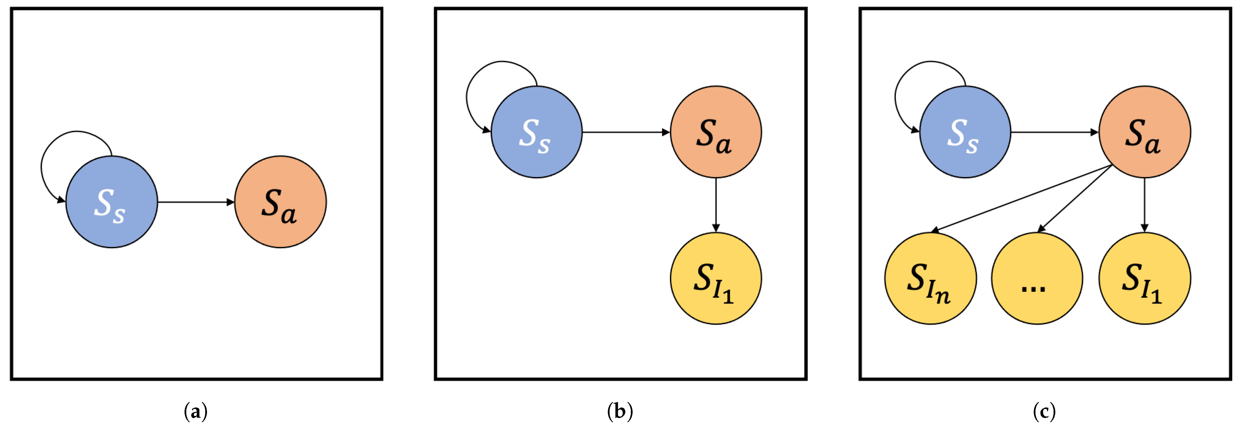
Figure 2 presents the overview of our model. We define a steady state $S_s$, in which the machine does not present any issue. This can happen for instance after a planned maintenance, in which all the critical components are checked and worn parts replaced. $S_s$ represents the state in which our model should recognize that the machine is in working order, does not present any issue, therefore it should not give any warning to the operator. Upon running, the machine may experience unseen states, in which the behavior of one or more sensors installed on the machine deviates from $S_s$. This is called an anomaly and it is represented by $S_a$. Note that at this stage the precise issue may not be known, hence our model will simply output that there is an anomaly, without necessarily specifying which one. This scenario is depicted in Figure 2a. Whenever an anomaly is detected, the system warns the operator for a possible issue on the industrial machine, giving the possibility to describe it, by detailing the specific issue experienced. This makes the model able to learn that the unknown anomaly which has just been experienced is now described in terms of kind, issue type and any other detail that the operator wants to use. In our model this translates into learning a novel state, called $S_{I_1}$, which represents a specific issue which may happen on the industrial machine. Note that $S_{I_1}$ is not defined a priori, but it is declared after the operator describes the first issue which is found on the industrial machine. At this stage, depicted in Figure 2b, the system is aware of the steady state $S_s$, which can lead to an anomaly $S_a$, and since it is now known also $S_{I_1}$, in case the same anomaly is found the system may recognize it. This happens since after having at least one described anomaly, the system upon the case an anomaly is found also tries to classify it against all the known issues, in this case only $S_{I_1}$. If the classifier matches the current anomaly with $S_{I_1}$, then it outputs the specific issue, hence not just an unknown anomaly. In case the current anomaly is not recognized among any of the previous ones, it again offers the operator the possibility to describe it as a novel one. This can lead to several anomalies described as specific issues by the operator, which can lead to the scenario we show in Figure 2c, where different issues are known to the system and analyzed in case any anomaly is found. Clearly, the number of issues and the data used to describe them is left to the specific scenarios, and operators need to be trained about this aspect.

3.2. Implementation

In this section, we detail the implementation of our model. Let $\mathcal{M}$ be the industrial machine on which we perform the predictive maintenance task, and ${\mathcal{S}}_{\mathcal{M}}=\{s_1,s_2,\cdots ,s_N\}$ be the set of N sensors through which we sense the machine dynamics.

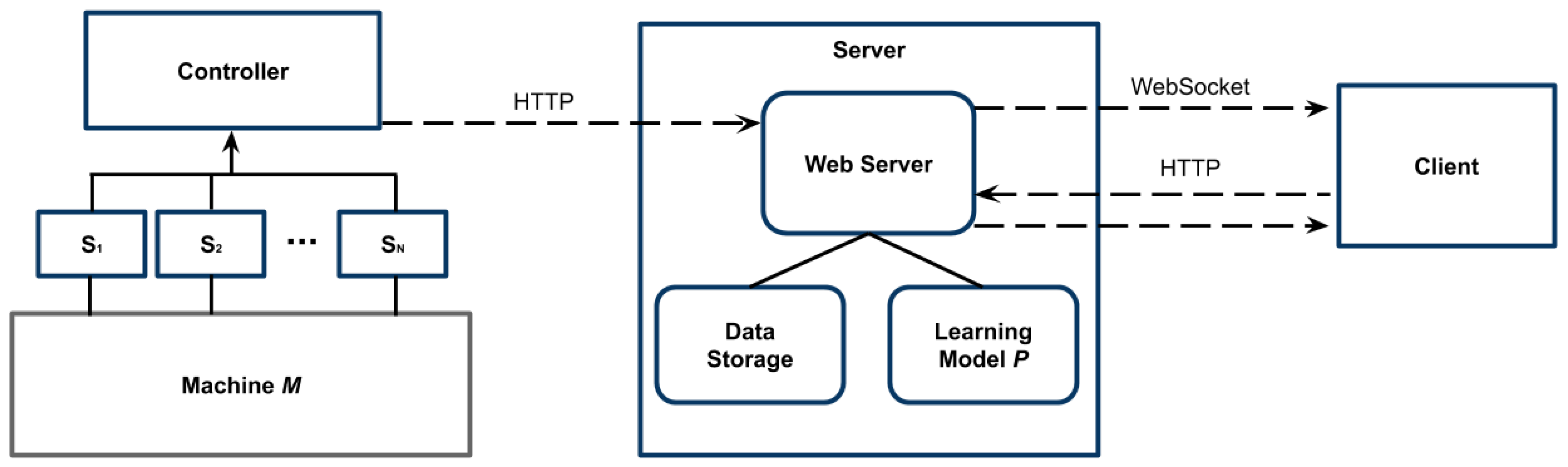
Figure 3 shows the architecture of the proposed system. The set of sensors ${\mathcal{S}}_{\mathcal{M}}$ can be directly connected to a collector, which can serve data through a local controller. As we already stated, $s_i$ can be anything, such as accelerometers, sound sensors, voltage sensors and so on and so forth. In particular accelerometers can be used to sense unusual vibrations, which may relate to parts not tightened together or excessive loads. Sound sensors may instead be used to assess whether sounds which were not present during normal operation of $\mathcal{M}$ are instead heard, thus potentially indicating malfunctions. Clearly many other sensors can be used, and their final choice depends on the kind of industrial machine on which it has to be performed the predictive maintenance task, and to the possible points of failure of it. However our framework is sensor-agnostic, meaning that it can adapt itself to different kind and number of sensors, and continuously learn new behaviors of $\mathcal{M}$. As a final note it also enables the system to scale, starting with a low number of sensors, and gradually adding new ones which add information to the model, thus specializing more on specific failures.

Communication is performed between the Controller or directly from the sensor $s_i$ with HTTP, through which each sensors $s_i$ reports the date it senses to a local server, running a web server which stores the data locally, and on which we deploy the learning model $\mathcal{P}$ described in the next section. We note that this architecture allows for different configurations in terms of network protocols used and sensors types. For instance, there may be more energy efficient communications if sensors communicate to the local controller through specialized M2M protocols, however this is out of the scope of this work and has to be determined depending on the specific scenario.

The web server is connected to a client, both with a WebSocket and with HTTP messages. The client is needed by the operator to interact with $\mathcal{P}$, and to be notified about possible issues which needs to be investigated further. In our experiments we have implemented the client on a tablet which we place aside of the industrial machine, but it may also be implemented on a mobile application or as a web application. Again this depends on the specific scenario and on the requirements of the application.

3.3. Learning Model $\mathcal{P}$

In this section, we describe the learning model $\mathcal{P}$, which is the main component which learns from the data obtained from the sensors, recognizes possible anomalies, and classifies such anomalies when operators describe the issues.

The learning model $\mathcal{P}=\{A,\mathcal{C}\}$ is built with two different components, the anomaly detector A and the classifier $\mathcal{C}$. The anomaly detector is run every T seconds, where T is the size of the sensing window. The specific features computed over the sensing window will be detailed in Section 3.4.

The anomaly detection model A is trained with a one-class SVM. This kind of model is able to train a base state and recognize novelties in the features. Thus, it is well suited for our case, as we can train it when the industrial machine is functioning properly, and let it recognize whenever any novelty in the data, which is an anomaly, is observed.

Whenever an anomaly is detected by A, we enter the $S_a$ state as depicted in Figure 2. The classifier $\mathcal{C}=\{C_1,\cdots ,C_N\}$ is a set of classifiers, each one trained on a specific anomaly. All the $C_i$ are defined as one-class SVMs, and each one of them is trained on a specific anomaly. Although one-class SVM models can be heavily parametrized, for our work we found that several configurations suited our scenario, mainly because the signals of the issues can be clearly distinguished with respect to the steady case. A deeper study on the SVM parametrization is left as a future work. Upon entering the state $S_a$, in case no specific anomaly has been previously found (i.e., $\mathcal{C}=\varnothing )$, the operator needs to describe the anomaly. Let i be the specific anomaly found, then the K previous windows on which A found the anomaly are used to train $C_i$, which is then appended to $\mathcal{C}$. The value of K depends on the time which passes between the start of the anomaly experienced by our system and its description by the operator. Therefore K can vary depending on how fast the operator is: in case the anomaly is described shortly after experiencing it K will be small, in case the operator takes more time K will be large. For sake of clarity, in our scenario the time needed was in the [30:90] seconds range, therefore it can lead to different K values depending on the size of the time window.

$\mathcal{P}$ now has the ability not only to detect anomalies, but also to recognize a specific one if the corresponding $C_i$ has been trained before. When the system is in the state $S_s$ and finds an anomaly, it then moves to state $S_a$. At this stage if $\mathcal{C}\ne \varnothing$, the sensed window which raised the anomaly is also tested against each $C_i\in \mathcal{C}$. Since the one-class SVM is able to detect the novelty of features with respect to those it has been trained with, in case $C_i$ considers the sensed window similar to the ones used to train it, then it also raises the specific anomaly i. In case no $C_i$ is able to correctly characterize the anomaly, we consider it as unseen before, therefore the operator has to label it so that a novel $C_i$ is trained and added to $\mathcal{C}$. In other words, A uses one-class SVM to identify deviations from the data and to identify anomalies, while each $C_i$ uses a one-class SVM to check whether there is no anomaly, meaning no substantial difference from the data on which $C_i$ has been trained on, hence classifying the issue.

We provide the pseudo-code of the algorithm we developed in Algorithm 1.

Algorithm 1: Anomaly detection and classification

At line 1 we read the data from the sensors, and compute the corresponding features into W, which is then tested for the anomaly at line 2. In case no anomaly is found the algorithm ends, waiting for the next data to analyze. In case an anomaly is found, we test W against all classifiers at line 7. In case at least one of them reports a known issue we output it at line 11. Conversely if no known issue is found, the output tells that no known anomaly is found. In the latter case, the operator may also describe the found issue so that the next time it is observed it is possible to directly identify it.

3.4. Feature Engineering

In this section, we describe the different features we collect from the raw data gathered from the sensors. More formally given a sensor i reading a signal ${\mathsf{\Theta }}_i$, we create windows of size T seconds, namely $W_i^T\left[j\right]$ which refers to the j-th window of the i-th sensor built with the sensing window of size T. We then compute 12 features to extract the signal dynamics. We compute basic statistical metrics such as the mean $\mu$:

$${\mu }_j^i=\frac{\sum W_i^T\left[j\right]}{|W_i^T\left[j\right]|},$$

(1)

the maximum of the window simply defined as:

$$ma{x}_j^i=max\left(W_i^T\left[j\right]\right),$$

(2)

and consequently the minimum:

$$mi{n}_j^i=min\left(W_i^T\left[j\right]\right),$$

(3)

and eventually the standard deviation:

$$\sigma =\sqrt{\frac{\sum {(x_k-{\mu }_j^i)}^2}{|W_i^T\left[j\right]|}},$$

(4)

where $x_k$ is a single measurement of window $W_i^T\left[j\right]$. These statistical metrics help to understand the shape of the signal, with respect to its variance over the time window and to spot possible peaks of it. For instance, for vibration sensor we may expect a rather low variance, while for a sound sensor it may be higher in presence of specific events.

We also compute the Fast Fourier Transform (FFT) of the signal as $FF{T}_j^i$, and the Power Spectral Density (PSD) of it, namely the $PS{D}_j^i$.

We also leverage the Peak defined as

$$Pea{k}_j^i=\frac{ma{x}_j^i-mi{n}_j^i}{2},$$

(5)

which models the difference between the maximum and the minimum value, hence it helps to understand how wide is the value span of the i-th sensor.

We also leverage the Root Mean Square (RMS), which is defined as:

$$RM{S}_j^i=\sqrt{\frac{1}{|W_i^T\left[j\right]|}\sum _{i=0}^{|W_i^T\left[j\right]|-1}{\left(x_k^i\right)}^2}.$$

(6)

The RMS is similar to the mean, but it better characterizes it when dealing with positive and negative numbers.

Having defined $Pea{k}_j^i$ and $RM{S}_j^i$ we can now compute the Crest Factor (CF) which is defined as:

$$C{F}_j^i=\frac{Pea{k}_j^i}{RM{S}_j^i},$$

(7)

and correspondingly the Kurtosis coefficient, which gives insights on how flat the distribution of values is, defined as

$$K_j^i=\frac{1}{W_i^T\left[j\right]}\sum _{i=0}^{|W_i^T\left[j\right]|-1}\frac{{(x_k^i-{\mu }_j^i)}^4}{{\left({\sigma }_j^i\right)}^4}.$$

(8)

In contrast to $K_j^i$, the $C{F}_j^i$ value enhances higher values. Hence, the two metrics complement each other, and used in conjunction help in better describing the signal.

We then compute the Skeweness (SK) of the signal, defined as:

$$S{K}_j^i=\frac{1}{|W_i^T\left[j\right]|}\sum _{i=0}^{|W_i^T\left[j\right]|-1}\frac{{(x_k^i-{\mu }_j^i)}^3}{{\left({\sigma }_j^i\right)}^3},$$

(9)

which describes whether the right and the left tail of the distribution of values are similar, or if the distribution is more skewed towards one of them.

Finally we compute the Entropy (E), used mainly to determine how diverse the signal is, defined as

$$E_j^i=\sum _{i=0}^{|W_i^T\left[j\right]|-1}P\left(x_k^i\right)lo{g}_{2}P\left(x_k^i\right)$$

(10)

These features are not computationally intensive to be computed, hence do not require extensive computational capabilities, making it possible to run the framework in real time and also on edge devices with limited capabilities. We provide evidence of this in Section 5.

4. Case Study

To assess the benefits of the proposed framework we tested it under three different data sources. This highlights how generalizable the model is, and its ability to adapt to different data sources and different data collection architectures. Moreover it also shows the possibility to run the model with a different number and type of sensors, crucial in this kind of scenarios, as every industrial machine present specific characteristics which have to be assessed with the appropriate sensors.

More specifically the three scenarios on which we performed our tests are the NASA dataset [7], a custom built prototype machine and a real industrial machine. Throughout these different scenarios we do not modify in any way the general framework. Clearly different kind of failures are experienced and different sensor readings have to be accounted for, hence the model adapts itself to these issues as the operators describes them.

4.1. NASA Dataset

The NASA dataset [7] is related to the monitoring of the different bearings of an engine. The bearings are monitored through accelerometers and the data is collected through a central entity. The dataset reports the total time of monitoring and the breaking point of the component. Due to the nature of the dataset, we will not perform classification of the different issues on this dataset. Instead we will leverage it to understand the speed of anomaly recognition of our proposal, starting from the point in which it is noticeable the potential issue.

4.2. Prototype Machine

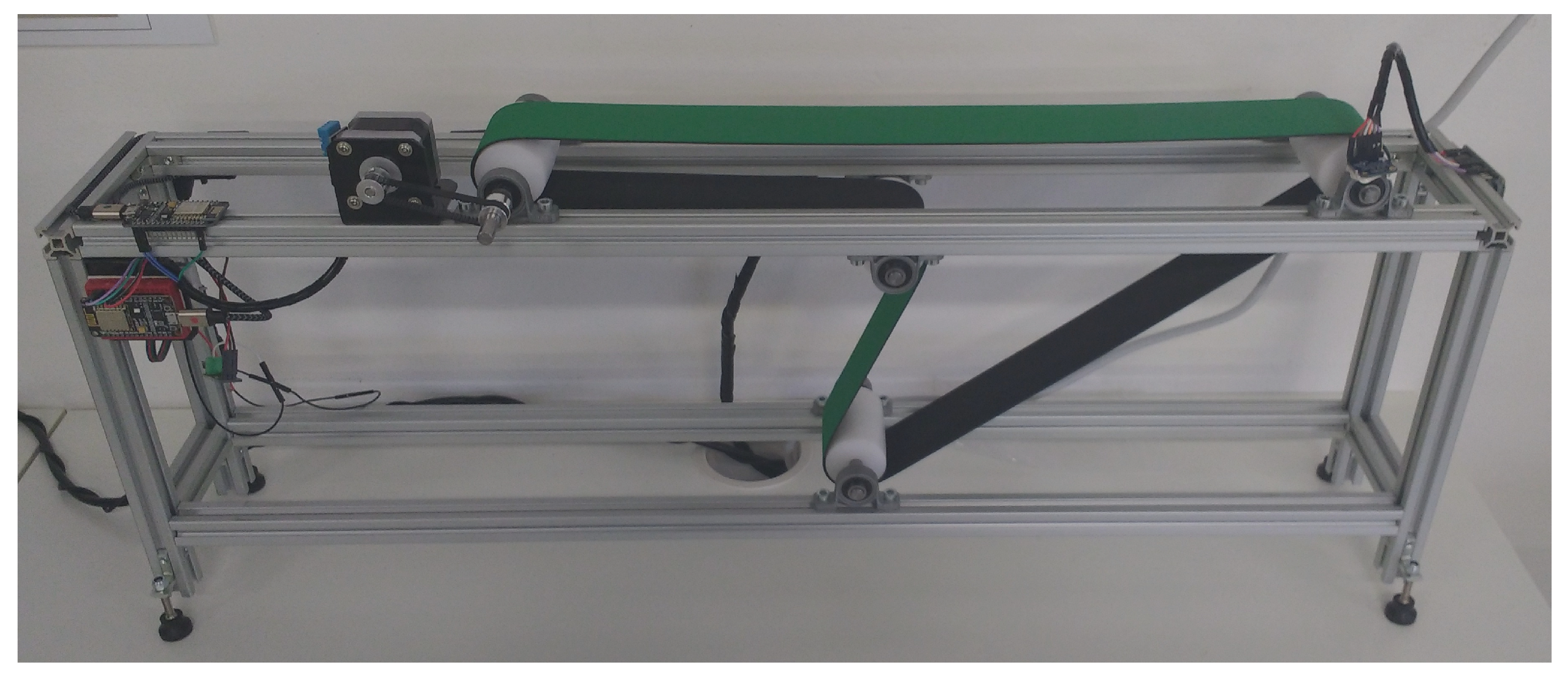
Figure 4 shows the general architecture of our prototype, and also highlights the sensors we used in our experiments. More precisely, for the purpose of this study we collected vibration patterns with an accelerometer, the temperature of the engine and the current drained. Clearly the set of sensor is suitable only related to the specific industrial machine which has to be monitored. This has to be designed a priori by specialized individuals, so that appropriate sensors can be installed and configured to check the key components of the industrial machine.

The prototype machine is built so that the belt spins moved by an engine installed on top of it. The machine is leveled with the help of four feet, which can be raised or lowered according to the surface on which the industrial machine stands. This simulates a typical industrial environment, in which there is a belt carrying pieces to the next step of the manufacturing process.

We tested three possible issues on this machine which are:

• Untightened screws: this may happen as the industrial machine vibrates, hence it may make the screws to become loose.
• Increased friction on the belt: this may happen when there is not enough lubricant or the belt rotor becomes dirty.
• Loose foot: as the industrial machine has to be stabilized, the feet are adapted to level the industrial machine. If any of these become loose, then the machine is not leveled anymore, hence vibrations and rotations will behave differently.

4.3. Production Machine

The last dataset we use is collected from a real industrial machine, pictured in Figure 5, whose task is to fold plain paper into boxes. These boxes are then placed on a conveyor belt and eventually moved to the next stage of the process. The machine itself, according to the owner, presents one critical component, which takes care of the alignment of the conveyor belt. In case it is not perfectly aligned boxes may come out with various defects such as open sides, bumps and scratches. Therefore we decided to monitor such component, which is attached to the machine through two screws, one on the left and one on the right. If these screws become untightened, then the vibrations start to increase on one side or the other, requiring manual maintenance. We then installed two accelerometers, each one attached to any screw, to monitor left and right vibrations. This issue is experienced from time to time, as the vibrations of the machine naturally make the screw loose, therefore resulting in possible misalignment of the conveyor belt. After installing our system, which was also enriched with a graphical user interface which can be seen on the left of Figure 5, we explained how the system works and what are the responsibilities for the personnel. We then double checked that the screws were correctly tightened, and we started to run the system which learnt the steady state. Upon anomalies, the operators had the opportunity to verify the issue, and instruct the system on the specific problem found. For this test, operators identified two levels for the same issue, related to how much the screw is loose.

5. Numerical Results

In this section, we present numerical results on the evaluation of our framework using the datasets described in Section 4.

5.1. Reaction Time

This analysis covers the ability of the model to react fast enough to the anomaly. To model it we used the P-F curve, which describes the state of health of the equipment over time, and highlights the time in which a potential failure started to be noticed, and the time in which such issue becomes a functional failure as shown in Figure 1.

For this test we used the NASA Bearing dataset, as it contains test to failure experiments, which enable us to understand how fast our proposal would react in presence of a failure.

There are three different tests in the dataset: for test 1, bearings 3 and 4 are the ones which present issues, test 2 only has bearing 1 with defects, and finally test 3 presents an issue in bearing 3.

As it can be seen from

Table 1. Reaction times.

Test ID	Bearing ID	Warning Time (Since p.f.)	Failure Time (Since p.f.)
1	3	227 min	5800 min
1	4	145 min	5800 min
2	1	44 min	4330 min
3	3	21 min	53,430 min

, the model reacts fast upon the potential failure, well ahead of the failure time. Due to the nature of the dataset, in this case our proposed model identifies an anomaly without classifying it hence only A is tested. It learns from the initial data fed to it, and whenever the potential failure starts to be noticeable, it detects the anomaly in the data. This happens regardless of the test ID, and regardless of the specific bearing presenting the issue, demonstrating the adaptability of our model. This test shows the ability of the model to react quickly to the experienced issue, allowing operators to perform maintenance on the industrial machine.

5.2. Varying Dataset Size

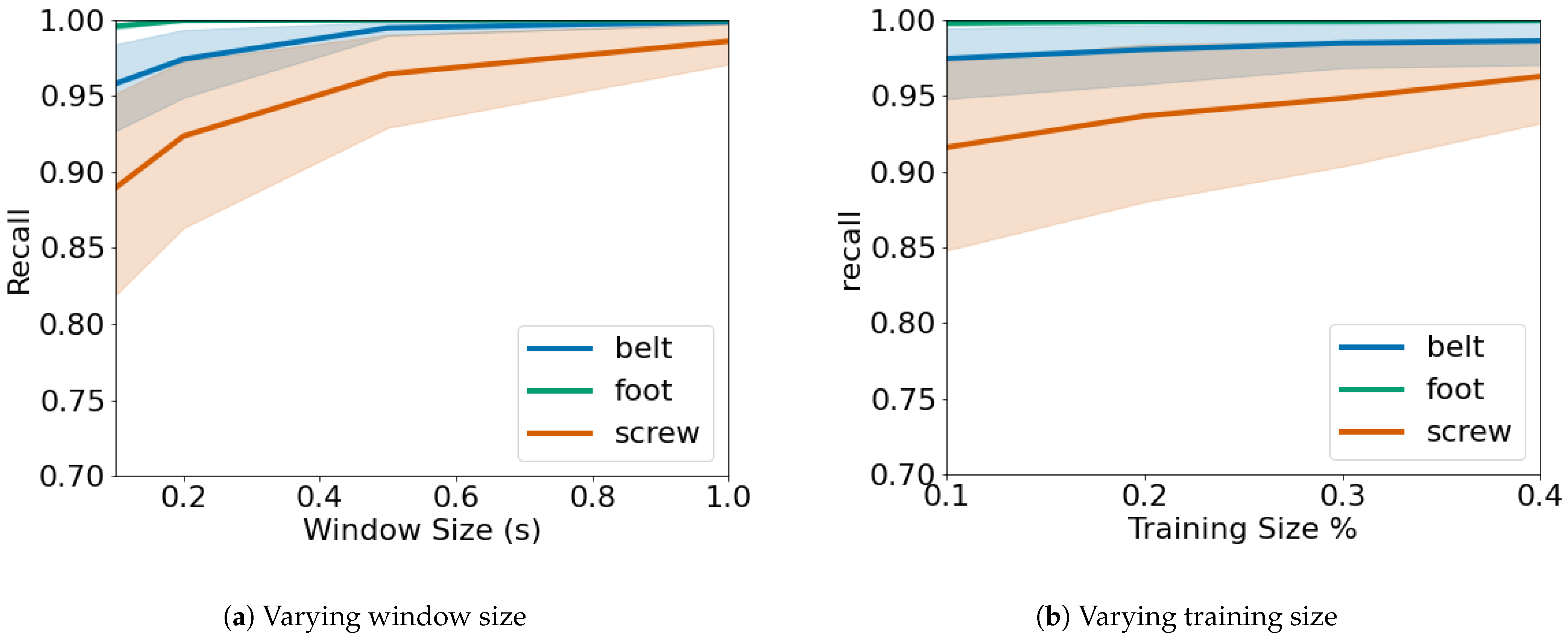
Figure 6 shows the recall of the classifier algorithm in classifying different issues, versus the window size in Figure 6a and versus the training size in Figure 6b.

If we look at Figure 6a, we can see that the greater the window size, the better the recall results. With a window size of 1 s the recall is almost 1 regardless of the issue type. This happens as longer window sizes present more signal characteristics, which makes it easier to assess how the signal is, hence making it easier to correctly detect any anomaly. We can also observe that some issues, such as a loosen machine foot, are easier to be recognized compared to others such as an untightened screw. This may indicate better sensor placement, a more suitable sensor type, or in general that some issues are easier to be recognized than others. However even with the smallest window size that we tested, equal to 0.1 s, all three issues achieve a recall greater than 0.85, which confirm the benefits and the good performance of our proposal.

Figure 6b presents a similar behavior, in which a larger training size results in a higher recall by the classifier. This result also confirms that issues are different regarding the easiness of being classified, as again the loose machine foot achieves top results even with the smallest training size. It is also worth noting that in this scenario even the highest values are able to provide a satisfiable results in a short time frame, with a relatively small percentage of the dataset used for the training of the classifier.

5.3. Varying Issue Level

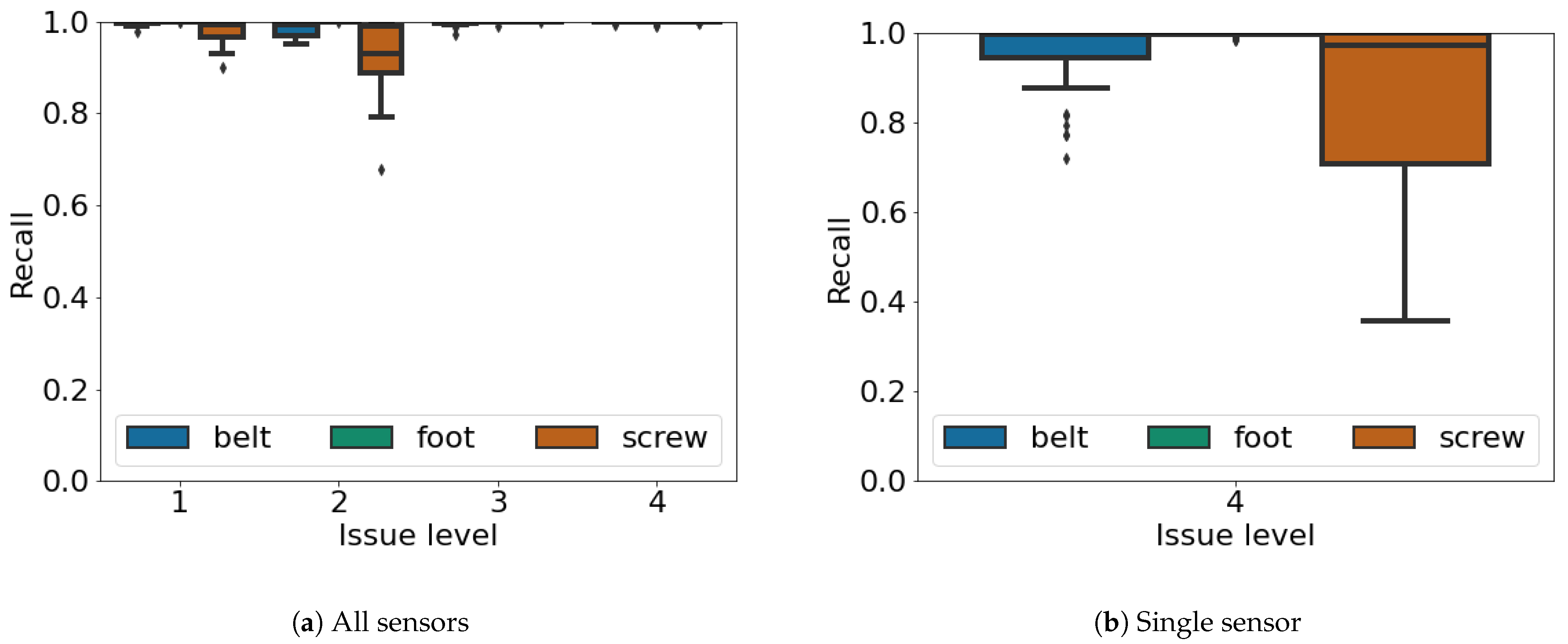
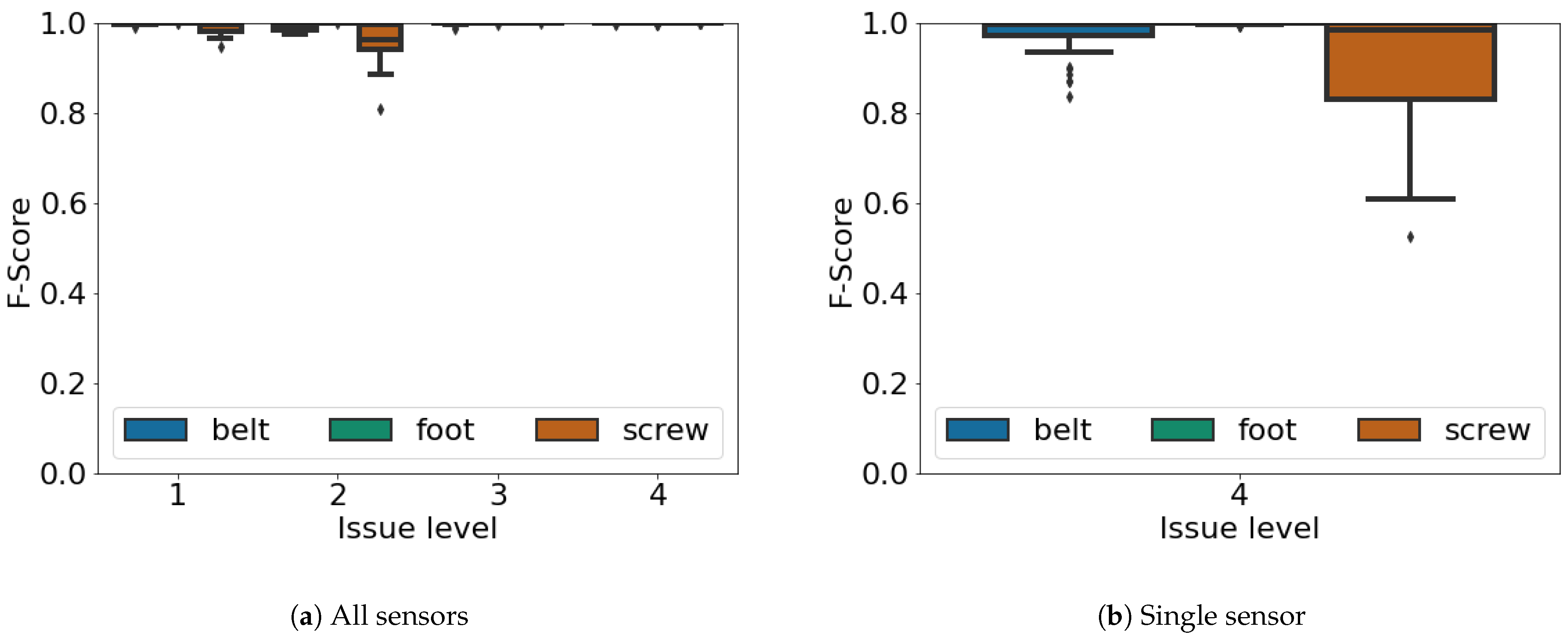
Figure 7 and Figure 8 present the recall results and f-score measures for different issue levels when using all the sensors available (Figure 7a and Figure 8a) and when using only the accelerometer (Figure 7b and Figure 8b). When using all the sensors each issue occurs with a different level, going from the lowest (i.e., 1) which is the one in which the issue is less severe, going up to the highest (i.e., 4) in which the specific issue is at the most severe level, right before a functional failure. For instance, considering the screw, a level of 1 means that the screw is slightly untightened while a level of 4 means that the screw is almost falling off. We can again see that the loose foot is the easiest issue to be classified, achieving top results regardless of the issue level and whether we are using all the available sensors or just a single one. This is related to the fact that a loosen foot unbalances the whole industrial machine, hence making quite peculiar sensor readings. Furthermore, the misaligned belt provides good results, as the vibrations are quite easily recognizable. Eventually the screw, as also observed in Figure 6, is the most challenging issue to be classified, as it is also the smallest part of the industrial machine. The results are however similar between the recall and the f-score, showing a good performance regardless of the configuration and of the specific issue. We also note that for any issue, a level of 1 refers to the beginning of a potential failure according to the P-F curve of Figure 1. Hence the ability to correctly identify a level one issue confirms again the fast reaction of our proposal in the presence of failures. However both Figure 7 and Figure 8 consider a matched class only when the specific issue is recognized, at the level in which it is experienced. In other words for our experiments if the classification reported the correct issue, but a wrong issue level, we considered it as wrong. We posed ourselves in this challenging scenario to show the real performance of our system, also considering that in some specific scenarios knowing the exact issue level may be compulsory for planned ordinary maintenance, as low level issues may be better tolerated by the industrial machine.

5.4. Correctness of Classification

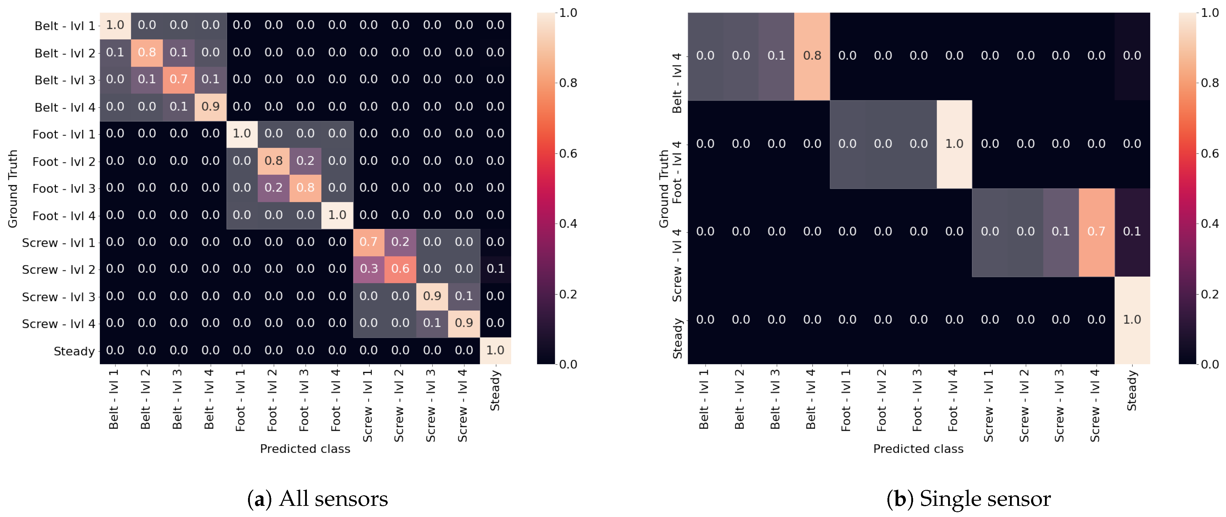
As we noted recognizing the precise issue level is more challenging than just recognizing the piece of equipment which needs maintenance. For this reason we now show the confusion matrices, which are depicted in Figure 9a for the case in which all sensors are used, and in Figure 9b for the case in which only one sensor is used. We have highlighted the parts of the matrices in which all the classifications refer to the same issue with white, regardless of the level of it. As it is possible to see the highlighted parts of the matrices are the only ones in which there are values greater than 0, meaning that even if the precise issue level is not found, still the classifier is able to recognize the issue type. We can also observe that in general the highest miss-classification is between adjacent levels, as they may present similar signal behaviors. This is true for instance for the belt, in which level 2 and 3 are sometimes classified as the other one, the same goes for the foot, while the screw considers level 1 and 2 similar, and the same goes also for levels 3 and 4. This confirms the almost perfect classification with respect to the issue itself, while determining the exact issue level is a more challenging task, although we have shown in the earlier results that the performance still remains high.

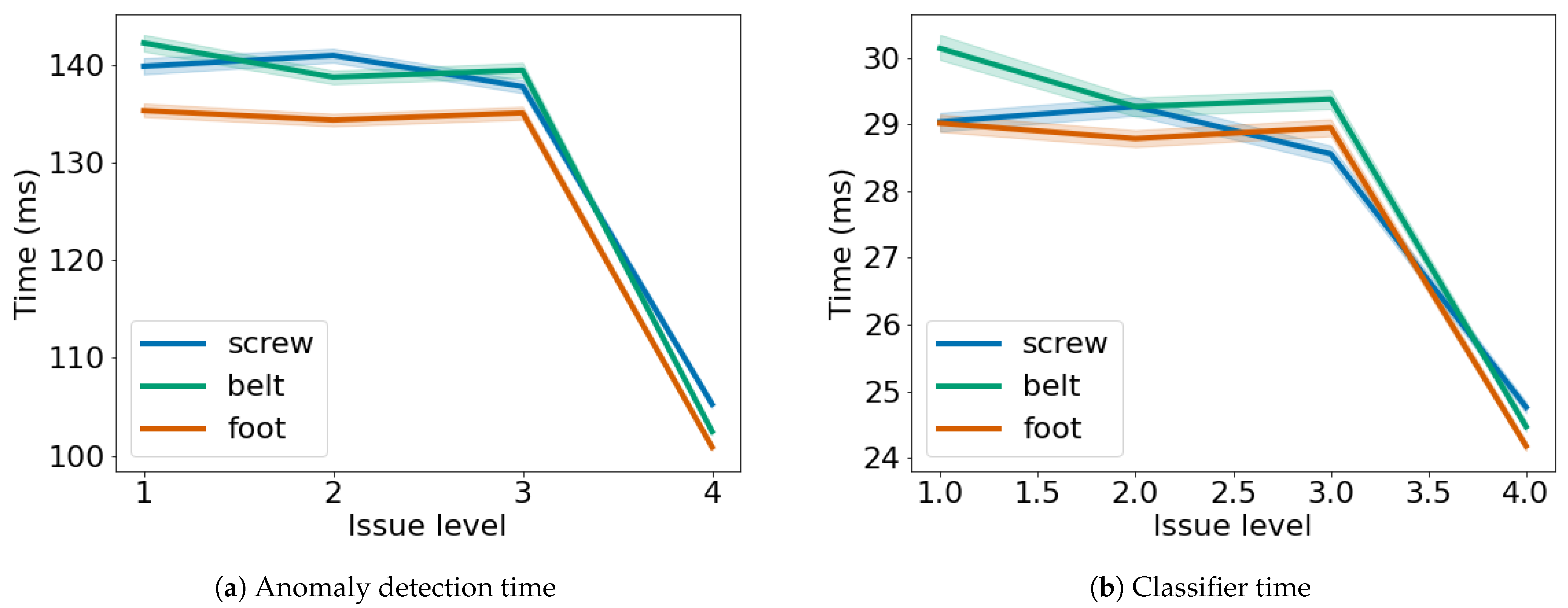
5.5. Computation Time

In Figure 10a, we also show the time needed to perform the anomaly detection and the time needed for the classifier to classify the sample is shown in Figure 10b. It is worth noting that the classifier will not run in case the anomaly detector will not detect any anomaly in the data. As it can be seen, the time needed to compute either the anomaly detection or perform the classification is quite small. In both cases when observing a maximum level issue, both the anomaly detection and the classification take less time. This happens as the sample present more peculiar characteristics, therefore the windows are easier to be classified hence the reduced time.

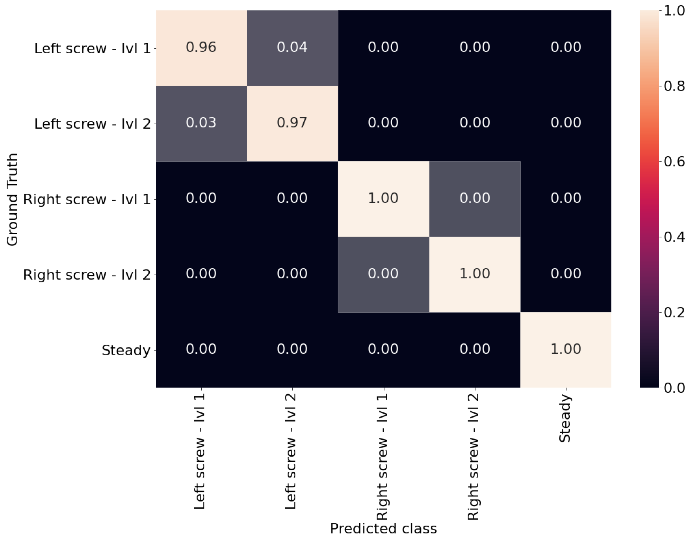
5.6. Real World Experiment

Figure 11 shows the experiment we performed on the real production machine to test our system in real working conditions. After running extensive tests we evaluated the performance of the system, which is presented in Figure 11. As we already saw in Figure 9a the accuracy of the system is satisfactory, with the only errors which are experienced for the same issue at different levels. It is also possible to see that the right screw achieves better results compared to the left screw: we investigated this, and we found that the left screw is closer to the conveyor belt engine, which also vibrates during operations. This may confuse the algorithm in recognizing the precise level of the issue, as the vibrations from the engine may alter those experienced by the screw. However, we can also see that the steady state is recognized perfectly, meaning that no unnecessary maintenance is requested to the operators.

6. Discussion

In this section, we discuss some of the possible integration of our architecture in different popular IoT scenarios, such as the Social Internet of Things (SIoT) [28] and in Multi-IoT scenarios (MIoT) [29,30] and in Smart Homes (SH) [31].

In the SIoT devices, actuators and sensors mimic a social network, by creating connections and improving the overall status of the system. The overarching idea of the system is to bring social networking to devices, by connecting them and making them able to provide novel collaborative services. At first in SIoT there is a challenge related to the relationship of different devices [32]. As sensors are deployed over an industrial machine, there is the need to understand groups and connections among them. In other words, in our scenario sensors closer to each other are more likely to form a group, meaning that they can provide data about a similar phenomenon, hence to understand a possible issue in the industrial machine. The SIoT can also manage the different relations among devices: for instance in our scenario it is possible that a causal relation between different issues exists. In other words an issue which is not handled may unleash another issue, hence it is possible to understand relations between issues and sensors. Practically this means that the central system, upon experiencing an anomaly, may advise the user to check also for other potential issues which are not still observed, but may probably be experienced in the future as a consequence. An interesting case is also reported in [33], where the authors use social relations between devices to provide a predictive maintenance service through a digital twin with distributed ledger. The SIoT is also leveraged for predictive maintenance tasks in [34], where the authors estimate the Remaining Useful Life (RUL) of the components by providing an ontological representations of them. In general in SIoT it is possible to integrate the system we just presented and leverage on some of the peculiar aspects of SIoT, like the relationship between devices, and the possibility to understand causal effects.

Another scenario is the Multi-IoT (MIoT) [29,35], which is a specific case in which the focus is on a high level of several IoT devices. MIoT scenarios are data driven and independent from the specific technology used, as the focal point is on the content exchanged by devices. MIoT is particularly useful when considering networks of networks, which may share data in order to achieve a customized service. Closer to the work in this paper is [36], where the authors specifically tackle the problem of anomaly detection in MIoT scenarios. Specifically in such article there is an interesting discussion on two separate aspects, which are the “forward problem” and the “inverse problem”. While the former is the classical anomaly detection, in which from a set of data the goal is to find whether such data presents an anomaly or not, the latter case is more difficult as it tries to understand what has caused such anomaly. In the context of Industry 4.0, this would open up the possibility to understand which component is faulty hence to speed up maintenance operations.

For Smart Home (SH) appliances, anomaly detection and predictive maintenance tasks can be customized to a number of different scenarios and to cover a plethora of purposes [37,38].

The works in [39,40] addressed the problem of Assisted Living (AL), where people with disabilities live in their SH and an intelligent system monitors their behavior for possible discrepancies. This requires the system to understand, as in our case, a set of variables and parameters for which the system is considered to be in a steady state, which for the AL scenario can be considered a safe state, meaning that the assisted person is not in danger. By constantly monitoring the changes in data and human behavior it is then possible to spot anomalies. This is done in [40] by monitoring temporal relations between actions, with associated probabilities of transitioning from one activity to another, and therefore identifying probabilistically those transitions which were seldom experienced in the past. This may raise a notification to the caregiver, which can act promptly to help the assisted human reacting to the anomaly identified. Similar to what we do, the caregiver may also inform the system about the specific issue, so that in the future it will be recognized not as an anomaly but rather as a specific problem, hence possibly unleashing a more tailored intervention. A similar approach is also studied in [41] where the authors use a clustering technique to understand anomalies such as inactivity or too long activities in SH thanks to unobtrusive sensors. Another wide branch of research is devoted to security models, to assess whether network operations and accesses can be considered as normal or are instead to be considered as an anomaly [42,43,44]. In [44], the authors consider an Hidden Markov Model which models the normal behavior of an SH, and are able to recognize attacks with a high accuracy. In the specific domain of AL [42] analyzes potential attacks on IoT devices used by elderly people by monitoring unusual behaviors. Closer to this work is [43], where the authors provide different levels of anomaly detection, from an unknown unusual behavior to a properly classified issue. In this case the system presents at first anomalies when experiencing unusual behavior, and as it learns novel issues it presents a more precise classification of them.

In any of these scenarios there is the possibility to assess an anomaly at first, and when experiencing it humans can describe the specific anomaly, so that the system can learn and in the future may better inform the user about the issue. IoT networks have been adopted in many different scenarios, and whenever it is challenging to obtain data to train a classifier model in advance, and the system can allow a two step recognition (i.e., an anomaly at first, which is eventually described), the system we have just present can fit.

7. Conclusions and Future Challenges

In this paper, we have shown a predictive maintenance model which does not require an initial dataset to be trained on. Instead it learns by observing an initial steady state, and then it detects anomalies in the data, while also classifying issues already seen. The model is also not bound to any specific set of sensors, thus making it adaptable to a plethora of different use cases.

We have shown that our model solves two important challenges in this domain: (i) it does not require an initial dataset, which is unfeasible to obtain in a real scenario; (ii) it does not need to know in advance the number nor the description of the issues to be recognized.

We have tested our proposal on three different datasets, to show its adaptability to different scenarios, sensors and sampling frequency. In all three datasets the model performed well, achieving an almost perfect classification on the real industrial machine also due to the reduced number of classes. Clearly, increasing the number of classes would also change the performance figures of it. However, we also argue that these models may be better leveraged when they have to monitor a specific component rather that the whole machine, hence also reducing the set of possible issues. This is also a planned future work on this topic, in scenarios where there are several sensors which monitor different components. There, we want to investigate whether having separate smaller models, which only focus on a specific part of the industrial machine would be better compared to having a unique model which monitors everything. In such a scenario, we have to extend our model by enabling the possibility for it to split and only focus on the given components, and we will also leverage multi class classifiers.