Abstract
There are many studies in the scientific literature that present predictions from parametric statistical models based on maximum likelihood estimates of the unknown parameters. However, generating predictions from maximum likelihood parameter estimates ignores the uncertainty around the parameter estimates. As a result, predictive probability distributions based on maximum likelihood are typically too narrow, and simulation testing has shown that tail probabilities are underestimated compared to the relative frequencies of out-of-sample events. We refer to this underestimation as a reliability bias. Previous authors have shown that objective Bayesian methods can eliminate or reduce this bias if the prior is chosen appropriately. Such methods have been given the name calibrating prior prediction. We investigate maximum likelihood reliability bias in more detail. We then present reference charts that quantify the reliability bias for 18 commonly used statistical models, for both maximum likelihood prediction and calibrating prior prediction. The charts give results for a large number of combinations of sample size and nominal probability and contain orders of magnitude more information about the reliability biases in predictions from these methods than has previously been published. These charts serve two purposes. First, they can be used to evaluate the extent to which maximum likelihood predictions given in the scientific literature are affected by reliability bias. If the reliability bias is large, the predictions may need to be revised. Second, the charts can be used in the design of future studies to assess whether it is appropriate to use maximum likelihood prediction, whether it would be more appropriate to reduce the reliability bias by using calibrating prior prediction, or whether neither maximum likelihood prediction nor calibrating prior prediction gives an adequately low reliability bias.
1. Introduction
We consider the use of univariate parametric statistical models for generating predictive probability distributions for out-of-sample data. We restrict our discussion to continuous models, and we assume that the training data are independent. One way to create predictive probabilities in this context is to calculate point estimates of the parameters of the statistical model. Predictions can then be generated by substituting the point estimates of the parameters into the model in place of the real but unknown parameter values. We call this approach point estimate prediction. The prediction may consist of densities, probabilities, quantiles, random deviates, or other quantities related to the distribution. Methods for making point estimates of the parameters include maximum likelihood, method of moments, L-moments and probability weighted moments (PWM), among others, although maximum likelihood appears to be the most commonly used. Point estimate prediction has been used in many hundreds of papers in the scientific literature and continues to be widely used. In climate science, in particular, assessments of the probabilities of extreme events, and of the impact of climate change on extreme events, are often made using point estimate predictions. Recent examples include assessments of probabilities of extreme wind speeds in Europe [1], the possible impact of climate change on Canadian wildfires [2], the changing probabilities of dam overtopping [3] and the changing probabilities of heatwaves [4]. We cite a dozen further examples in Appendix B.
1.1. Parameter Uncertainty
However, a disadvantage of point estimate prediction is that it does not account for uncertainty around the estimated parameter values and does not propagate that uncertainty into the prediction. It has been noted by various authors that this leads to predictions that are too narrow and tail probabilities that are underestimated. For example, to quote Bernardo and Smith [5] (page 483): “We should emphasize...that the all too often adopted naive solution of prediction based on the ‘plug-in estimate’...usually using the maximum likelihood estimate, is bound to give misleadingly overprecise inference statements about y, since it effectively ignores the uncertainty about theta.” To quote Geisser [6] (page 17): “…introducing maximum likelihood estimates for the mean and variance…results in estimated prediction intervals that are too tight in the frequency sense.”
Quantitative assessments of whether prediction methods are able to generate reliable probabilities can be made using a method we refer to as reliability testing. In reliability testing, simulations over multiple training datasets are used to assess whether predictions of the exceedance quantile are really exceeded 10% of the time, and similarly for other quantiles. In this testing, we refer to the intended exceedance probability ( in the previous sentence) as the nominal probability (NP: a table of all abbreviations used is given in Appendix A). Other authors have variously referred to this as the required probability, the specified probability or the model probability. We refer to the relative frequency with which out-of-sample testing data exceeds the predicted quantile as the predictive coverage probability (PCP) or just the coverage probability (CP). Other authors have referred to this as the coverage probability or the true probability. We then refer to a prediction method for which the PCP matches the NP, as one may hope it would, as being reliable or well-calibrated. This definition of reliability and calibration is widely used for the evaluation of weather forecasts [7] and, in machine learning, for the evaluation of various types of prediction [8].
1.2. Background on Maximum Likelihood Reliability Bias
A number of previous authors have quantified the reliability of point estimate predictions using reliability testing. Gerrard and Tsanakas [9], in Table 1, give results for the reliability of maximum likelihood predictions for the exponential, Pareto, normal and log-normal distributions. They consider four sample sizes, from to , and NPs of , and . Blanco and Weng [10], in Table 1, give results for the reliability of both maximum likelihood and method of moments predictions for the Gamma (for four different parameter settings), normal and log-normal distributions, and for maximum likelihood predictions for the exponential and Pareto distributions. They consider a sample size of , and NPs of , and . More recently, Jewson et al. [11] give results for the reliability of maximum likelihood predictions for the exponential, Pareto, normal, log-normal, logistic, Cauchy, Gumbel, Fréchet, Weibull, generalized extreme value (GEV, GEVD) and generalized Pareto (GP, GPD) distributions, for method of moments predictions for the normal and for PWM predictions for the GEVD. They consider a sample size of , and a range of NPs from to . They also explore the impact of different sample sizes and parameter settings on the reliability of GEVD and GPD predictions and evaluate reliability for a number of models that include one or more predictors.
The results from these studies show that: (a) predictions generated using maximum likelihood, method of moments and PWM all underestimate tail probabilities; (b) the tail underestimation is larger for smaller sample sizes; (c) the tail underestimation is larger, in a relative sense, further into the tail and (d) the tail underestimation is larger when predictors are included.
1.3. Background on Objective Bayesian Prediction
Various studies have assessed whether objective Bayesian methods can be used to generate predictions with lower reliability bias than point estimate predictions. Severini et al. [12] show that, for a class of statistical models that we will refer to as the homogeneous models (defined in Section 2 below), using a prior known as the right Haar prior (RHP) gives predictions with exactly zero reliability bias. The Severini et al. [12] result is discussed in Gerrard and Tsanakas [9] and Jewson et al. [11]. Jewson et al. [11] then also consider a number of inhomogeneous models and show that for the models they consider, the reliability bias can be reduced relative to maximum likelihood prediction, but not eliminated, using carefully chosen priors. They give the name ’calibrating prior prediction’ to any objective Bayesian method in which the prior is chosen to improve the predictive reliability.
1.4. Study Objectives
The Gerrard and Tsanakas, Blanco and Weng, and Jewson et al. papers cited above include tables and graphs that show the size of reliability bias for various models and prediction methods. They are useful for understanding the characteristics of these prediction methods. However, they are not particularly useful as reference material, since they only consider a few specific cases and a few specific combinations of sample size and probability. In this paper, we extend these previous results to a much larger number of cases. In particular, we cover all combinations of sample sizes from to and NPs from to , for 18 different statistical models. We present our results as charts that can be used as a reference for estimating maximum likelihood, method of moments, PWM and calibrating prior prediction reliability bias as a function of sample size and NP.
These charts have two specific uses. First, they can be used to interpret results from studies in the scientific literature that have used point estimate prediction. If the reliability bias is small, that may lead to more confidence in those results. Conversely, if the reliability bias is large, that may lead to a reassessment of the implications of the results, and may suggest that some results would benefit from recalculation. The reliability bias from the charts can, in some cases, also be used to generate corrections to previous results, as we discuss below. Second, the charts can be used to help design future studies, in that they can be used to assess whether point estimate prediction is likely to be appropriate. If it is concluded that the reliability bias due to the use of point estimate prediction would be too large, then calibrating prior prediction can be considered instead.
In Section 2, we describe the simulation method that we use for generating our reliability results and give details of the calibrating prior prediction method. In Section 3, we illustrate point estimate prediction reliability bias for some simple cases and explore the impact of various factors on the size of the reliability bias. We then present reliability bias reference charts for point estimate and calibrating prior predictions, which are the main output of this project. In Section 4, we discuss our results, and in Section 5, we draw conclusions.
1.5. Study Limitations
There are a number of limitations to our study. We only cover 18 statistical models out of the infinite universe of possible statistical models. We also only cover independent univariate training data. For dependent univariate training data, more complex models that consider the dependency structure would need to be considered. The basic ideas would, however, remain the same. For multivariate data, Severini et al. [12] discuss some examples. However, reliability testing for multivariate models is complex and requires somewhat different methodologies to those that we present here.
2. Methods
We now discuss the reliability testing simulation method we use for our analysis, whether the results depend on the true parameter values, why we consider reliability bias rather than the sampling bias of probabilities and quantiles, and the calibrating prior prediction method.
2.1. Reliability Testing Simulations
We define the PCP for a given model as:
where is a vector of parameters for the model, is the NP, means probability, Y is the out-of-sample random variable that we are trying to predict, X is the training data random variable of sample size n, and is a predictive exceedance quantile, at the NP.
Following Gerrard and Tsanakas [9], one can evaluate the reliability bias straightforwardly using simulations as follows:
- Assign a model, a sample size n, and values for the model parameters , which we refer to as the true parameters.
- Given the true parameters, generate 100,000 sets of training data, each of the given sample size, using a random number generator for the model.
- From each of the training data sets, generate predictive quantiles at a number of NPs.
- Generate 100,000 testing values, using the same random number generator.
- Count the number of testing values that exceed each quantile prediction.
- Calculate the relative frequency of the number of values that exceeded each quantile prediction as a Monte Carlo estimate of the PCP and compare that estimate with the NP for that prediction.
This algorithm can be illustrated using simple computer code. The following R code applies the algorithm to the exponential distribution, for a true rate parameter of 3, a sample size of , and an NP of (corresponding to a non-exceedance probability of ). The predictive quantile is generated from a maximum likelihood estimate of the rate parameter. One might expect the testing data to exceed the quantile prediction 1% of the time, while this program shows that it actually exceeds the quantile prediction roughly 2.3% of the time, hence showing that the maximum likelihood predictive quantiles are not reliable and are too low.
---------------------------------------------------------------------------
ntrials=100000
count=0
theta=3
for (i in 1:ntrials){
x=rexp(n=10, rate=theta) # make the random training data
y=rexp(n=1, rate=theta) # make the random testing data
q=qexp(p=0.99,rate=1/mean(x)) # make an ML prediction of the 0.01 quantile
if(y>q)count=count+1 # compare testing data and prediction
}
cat("proportion=",100*count/ntrials,"\n") # look at the PCP (which is ~2.3%)
---------------------------------------------------------------------------
This algorithm for testing reliability has the benefit of being conceptually simple to understand. It is clear how it tests the ability of the prediction method to generate quantiles that relate directly to the relative frequencies of future values. However, we can make this algorithm more efficient as follows. We note that
In the algorithm, we can then replace steps 4, 5, and 6, with the alternative steps given below, as described in Jewson et al. [11].
- 4.
- Substitute each quantile prediction into the known distribution function based on the true parameters to calculate how often it will be exceeded. This gives the PCP for that quantile, for that single set of training data.
- 5.
- Average together the PCPs for all sets of training data to give an estimate of the overall PCP for each quantile.
- 6.
- Compare the estimated overall PCP with the NP.
The use of the distribution function instead of random samples for Y in this way converges to the same result but more quickly. The R code for this alternative version of the algorithm is as follows:
---------------------------------------------------------------------------
ntrials=100000
sump=0
theta=3
for (i in 1:ntrials){
x=rexp(n=10, rate=theta) # make the random training data
q=qexp(p=0.99,rate=1/mean(x)) # make an ML prediction of the 0.01 quantile
sump=sump+1-pexp(q,rate=theta) # evaluate the prediction using the true EDF
}
cat("PCP at %=",100*sump/ntrials,"\n") # PCP (which is ~2.3%)
---------------------------------------------------------------------------
The two algorithms described above test reliability using quantile predictions. We note that it is also possible to construct an algorithm that tests reliability using probability predictions, which is roughly as efficient as the first of the two quantile-based algorithms.
2.2. Dependence on Parameter Values
We now discuss to what extent the results from this testing depend on the true parameter values chosen, which depends on the model.
2.2.1. Homogeneous Models
First, we consider statistical models that have sharply transitive transformation groups, which we call the homogeneous models. For example, the set of transformations , for , form a sharply transitive transformation group over the normal distributions, and so the normal distribution is a homogeneous model. This type of model has been discussed by Fraser [13], Hora and Buehler [14], Severini et al. [12], Gerrard and Tsanakas [9] and Jewson et al. [11], among others. Alternative names for the homogeneous models might include the sharply transitive transformation models, the simply transitive transformation models or the exactly transitive transformation models.
The set of homogeneous models consists of location models, scale models, shape models, location-scale models, scale-shape models, and all these types of models with predictors on the parameters. It also includes simple transformations of these models, such as log-location models and log-location-scale models. Homogeneous models therefore include the exponential, some versions of the Pareto, the normal, the log-normal, the Gumbel, some versions of the Fréchet, the Weibull, the GEVD with fixed shape parameter, various other distributions, and all these distributions with predictors on the parameters.
For homogeneous models, the results of our reliability testing, in terms of the comparison between the NP and the PCP, do not depend on the true parameter values. As a result, we only have to generate reliability bias charts for one set of parameters. In a real modeling situation, the true parameters are typically unknown. However, since for the homogeneous models our reliability bias results do not depend on the parameters, the results we derive for these models apply even in the case where the parameters are unknown. A consequence is that for these models the reliability bias results we derive could be used as a way to correct the reliability bias in predictions from these models, and applying that correction would lead to predictions with zero reliability bias. Applying such corrections might be useful if the predictions cannot be recalculated, perhaps because the original data is not available. If the original data is available, it may be preferable to recalculate the predictions using methods that give lower reliability bias.
2.2.2. Inhomogeneous Models
Second, we consider distributions that do not have sharply transitive transformation groups, which we call the inhomogeneous models. For example, the GEVD is an inhomogeneous model. The transformation changes the location and scale parameters of the GEVD, but not the shape parameter. It leads to a transformation group, but the group action of the transformation group on the set of all GEVDs is not transitive. In fact, for the GEVD, there is no transformation that can change the shape parameter and that can be used to form a sharply transitive transformation group. One might say that GEVDs with different shape parameters are fundamentally different from each other, in a way that GEVDs with the same shape parameter but different location and scale parameters are not. This relates to the fact that a change in units can change the location and scale parameters but cannot change the shape parameter.
The set of inhomogeneous models includes the gamma, GEVD and GPD, among others. For inhomogeneous models, the results of our simulation testing depend on the parameter values for those parameters that are not part of any transformation group. For example, for the GEVD and GPD, the simulation results do not depend on the location and scale parameters since they are part of a transformation group, but do depend on the shape parameter, which is not. We therefore present GEVD and GPD results as a function of the true shape parameter. If the maximum likelihood estimate of the shape parameter is , then one can consider the reliability of predictions based on the true parameter value as being an approximation to the actual reliability bias. If the reliability bias is highly sensitive to the true parameter value, it may be a bad approximation. If the reliability bias is less sensitive to the true parameter value, it may be a good approximation.
Since the reliability bias for inhomogeneous models depends on the unknown parameter value, our reliability bias results for these models can only be used to correct reliability biases in an approximate way. As before, if the data is available, it may be preferable to recalculate the predictions using methods that give lower reliability bias.
2.3. Sampling Bias on Probabilities and Quantiles
The types of simulations we describe above can also be used, with slight modifications, to assess the sampling bias of estimates of probabilities and quantiles. The true parameters can be substituted into the distribution function for the model to derive target values for the probabilities and quantiles, and the predictive probabilities and quantiles can be compared with these target values. The sampling bias is the average of the differences between the predictions and the target over many trials. It is tempting to refer to the target probabilities and quantiles as the ‘true’ probabilities and quantiles, but they are only really true in the situation in which the parameters are known, in which there is no parameter uncertainty. Because the definition of the sampling bias of probabilities and quantiles compares against a target that does not include parameter uncertainty, it does not relate to out-of-sample prediction. In fact, probabilities and quantiles with zero sampling bias are generally not reliable as predictions, and predictive probabilities and quantiles that are reliable generally show non-zero sampling bias. For instance, an unbiased estimate of the return level is not itself necessarily a reliable return level, and so is perhaps not useful in a predictive sense. This is discussed in more detail in Jewson et al. [11].
2.4. Prediction Methods
We generate results for 18 statistical models. For all the models, we generate results using maximum likelihood prediction. For the normal distribution, we additionally generate results using method of moments prediction, and for the GEV, we additionally generate results using PWM prediction. For all 18 models, we also generate results using calibrating prior prediction, which we now describe.
2.4.1. Calibrating Prior Prediction
For situations in which reliable predictions are desired, but for which the point estimate prediction reliability bias charts show that point estimate predictions exhibit an unacceptably large reliability bias, the objective Bayesian method of calibrating prior prediction can be used instead.
For homogeneous models, the work of Fraser [13], Hora and Buehler [14] and Severini et al. [12] derives a calibrating prior prediction method that gives exactly reliable predictions. The prior is the right Haar prior of the model. Jewson et al. [11] give an explanation of this approach. For some homogeneous models (exponential, Pareto with 1 parameter, normal, log-normal), there are exact closed-form expressions for the predictive distribution. For other homogeneous models (logistic, Gumbel, Fréchet, Weibull), there are no exact closed-form expressions for the predictive distribution, and the predictive distribution has to be calculated in some other way. This can then introduce some lack of reliability, depending on how the prediction is calculated.
For the GEVD and GPD, which are inhomogeneous, Jewson et al. [11] show that using a prior proportional to the inverse scale parameter gives good reliability for medium and large sample sizes. There are no exact closed-form expressions for the predictive distributions for the GEVD and GPD.
2.4.2. Evaluation of Bayesian Predictions
For the cases in which there are no exact closed-form expressions for the predictive distribution, we must evaluate the calibrating prior predictions in some other way. The most widely used numerical methods for making Bayesian predictions are the various types of Markov Chain Monte Carlo (MCMC) algorithms. However, MCMC is too computationally expensive to generate the many millions of predictions required to create reliability charts. Instead, we use the DMGS method described by Jewson et al. [11], which, for generating quantile predictions, is several orders of magnitude faster than MCMC. The DMGS method uses approximate closed-form expressions given by Datta et al. [15]. Datta et al. derive the first two terms of an asymptotic expansion of the Bayesian prediction equation in powers of . The first term, which is , is a predictive distribution based on maximum likelihood estimates for the parameters, and the second term, which is , can be considered as an approximate correction to the maximum likelihood predictive distribution. Datta et al. give expressions for the predictive density and predictive quantiles. The expression for the predictive density can be integrated to give an expression for predictive probabilities.
The DMGS equations are valid under certain regularity conditions, which are satisfied by most of the models we are considering, but which are not satisfied by the GEVD and GPD. However, the equations can still be tested as an ad-hoc method for making predictions for these models. The equations for GEVD and GPD densities and probabilities fail at the maxima and minima of the random variables that occur for certain parameter values for these models, and hence are of little use. The DMGS quantile equation, however, does not fail for any value of probability and gives predictions with materially lower reliability bias than maximum likelihood when used with an inverse scale prior, as shown by Jewson et al. [11]. It is therefore a useful tool for making predictions for these models, even though it does not possess the precise asymptotic properties implied by the Datta et al. derivation.
2.4.3. Parameter Ranges
The DMGS equations rely on derivatives of the log-likelihood. However, for the GEVD and GPD, for extreme values of the shape parameter , these derivatives may be difficult to calculate. This can be managed in various ways. Jewson et al. [11] used finite difference calculations for the derivatives and found it necessary to eliminate all simulations with estimated shape parameters with an absolute value greater than 0.45. Eliminating simulations in this way introduces a bias in the estimates of the reliability bias, which may be material for small sample sizes and when the true shape parameter has an absolute value close to 0.45. In the current study, we have improved on this approach in two ways. First, we have used analytic expressions for the derivatives, generated using symbolic differentiation. This has allowed us to calculate the derivatives and apply the DMGS equations for all estimated shape parameters with absolute values less than 1. This greatly reduces the number of problematic cases. Second, when the estimated shape parameter has an absolute value greater than or equal to 1, we revert to maximum likelihood prediction, rather than eliminating the case entirely. Reverting to maximum likelihood gives a lower bias than would come from completely eliminating those cases. As a result of this different approach to dealing with extreme values of the estimated shape parameters, the results for the GEVD and the GPD in the present study show small differences relative to those in Jewson et al. [11], especially for small sample sizes and relatively extreme true shape parameters. This study should be considered more accurate.
3. Results
We now present the results from our simulations. We first present a number of investigations into the general nature of point estimate prediction reliability bias. We then describe the reliability bias charts for point estimate prediction methods, and finally we describe the reliability bias charts for calibrating prior prediction.
3.1. Investigating Point Estimate Prediction Reliability Biases
We now illustrate maximum likelihood, method of moments and PWM prediction reliability bias in various ways.
3.1.1. Normal Distribution Reliability Bias
Figure 1 illustrates maximum likelihood reliability bias for the normal distribution using a number of variations of the standard reliability diagram. We use a sample size of in order to exaggerate the reliability bias. Figure 1a shows a standard reliability diagram, in which the PCP is compared with the NP for the whole range of probability. There appears to be a reasonably good agreement between the PCP and the NP, in which the PCP only deviates slightly from the NP. For values of the NP higher than , the PCP is higher than the NP and vice versa. This indicates that the maximum likelihood prediction is too narrow and is underpredicting extremes at both ends of the distribution, as expected.
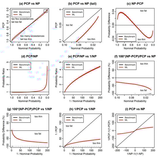
Figure 1.
Reliability test results for predictions of normally distributed test data, where the predictions were made using the same normal distribution with parameters estimated using maximum likelihood. (a) The predictive coverage probability (PCP) vs. the nominal probability (NP), with axes linear in exceedance probability. (b) The same, but for the upper tail. The small box in the upper right-hand corner of (a) illustrates the region covered by (b). (c) NP-PCP versus NP. (d) PCP/NP versus NP. (e) PCP/NP but now versus 1/NP. (f) 100 (NP − PCP)/PCP, for the upper tail. (g) 100 (NP − PCP)/PCP, but now versus 1/NP. (h) 1/PCP versus 1/NP. (i) shows 1/PCP − 1/(1 − PCP) versus 1/NP − 1/(1 − NP).
Figure 1b shows the upper tail from Figure 1a. Figure 1c shows the difference between the NP and the PCP. Figure 1c shows that the largest absolute differences between the PCP and the NP occur at NPs of and . Figure 1d shows the ratio of the PCP to the NP. In the upper tail, where the NP becomes small, this ratio becomes large.
It is helpful to illustrate reliability bias in the upper tail using a horizontal axis consisting of one over the NP. If the random variable corresponds to a single value in a fixed time interval, then this axis can be considered as a return period, and we will refer to this kind of axis as a return period axis. Using this axis covers the whole range of probability, but puts much more emphasis on the upper tail. Figure 1e shows the same results as Figure 1d but is transformed by this alternative choice of axis.
Figure 1f shows the difference between the NP and the PCP but expressed as relative errors as a percentage of the PCP. We see that the relative errors increase into the tail. Figure 1g shows the same results as Figure 1f, but as a function of a return period axis for the NP. Figure 1h shows both the PCP and the NP using return period axes. We refer to Figure 1h as a tail reliability diagram, since it focuses on the reliability of the tail. It illustrates clearly that the probabilities in the extreme tail are greatly underestimated. We will use the tail reliability diagram in many of our diagnostics below.
Finally, Figure 1i uses axes in which both the NP and the PCP have been transformed to . For small values of p, this is equivalent to a return period axis, and for large values of p this is equivalent to a return period axis for the return periods of non-exceedance. This is therefore a way to illustrate the reliability bias for both tails of the distribution in one plot.
The results in these various figures are reasonably typical for symmetric distributions, such as the t distribution, Laplace’s distribution and the logistic distribution.
3.1.2. Exponential Distribution Reliability Bias
Figure 2 is the equivalent of Figure 1 but for the exponential distribution, as an example of a one-sided distribution. The results are similar to those for the normal distribution for NPs below but are qualitatively different for NPs above , as shown in Figure 2a,c,i.
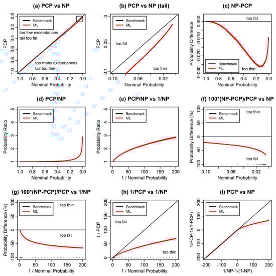
Figure 2.
As Figure 1 but for the exponential distribution.
3.1.3. Impact of Sample Size
We now consider the effect of sample size on the maximum likelihood reliability bias. Figure 3 shows the tail reliability diagram for the normal distribution for sample sizes from to . We see that the reliability bias reduces as the sample size increases, showing clearly that the reliability bias is a small sample size phenomenon, but that in the extreme tail it is still not negligible even for a sample size of .
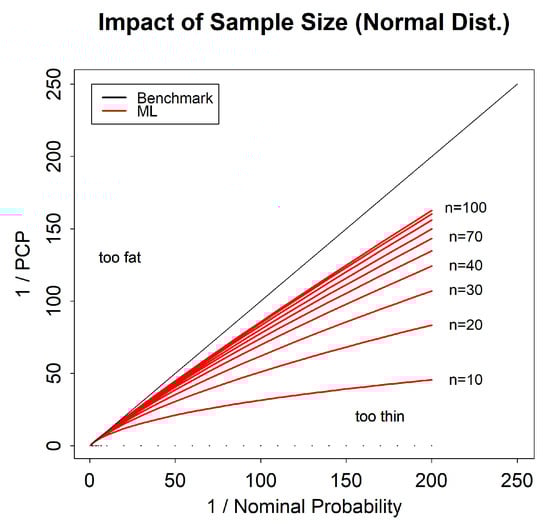
Figure 3.
Following Figure 1h, a tail reliability diagram for maximum likelihood predictions for the normal distribution, showing the impact of sample size.
3.1.4. Impact of Predictors
We now consider the effect of adding predictors to the parameters of a model on the maximum likelihood reliability bias. Figure 4 shows the tail reliability diagram for four versions of the GEVD: the GEVD with no predictors; with a predictor on the location parameter; with predictors on both the location and scale parameters, and with predictors on the location, scale and shape parameters. The predictor on the location parameter takes the form , with parameters and and a predictor . The predictor on the scale parameter takes the form , with parameters and and a predictor . The predictor on the shape parameter takes the form , with parameters and and a predictor . The addition of these predictors increases the number of parameters in the model. The figure shows that adding predictors to the model increases the reliability bias. This arises because of the larger number of parameters, leading to larger total parameter uncertainty. The true shape parameter is set to zero in all four cases.
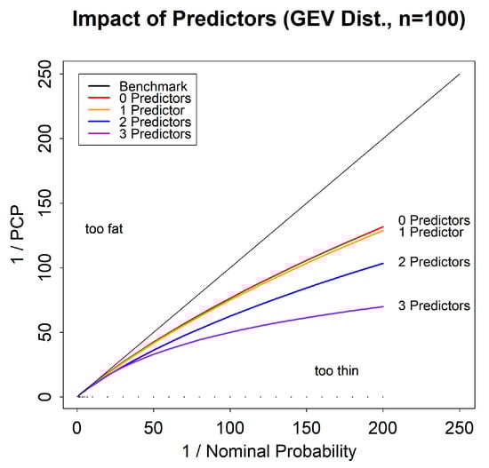
Figure 4.
Tail reliability diagram for maximum likelihood predictions for the GEVD with shape parameter = 0, showing the impact of including predictors.
3.1.5. Impact of Model
We now consider the maximum likelihood reliability bias for six different two parameter models. Figure 5 shows that, in general, different models will have a different reliability bias, even if they have the same number of parameters, but that some models (Gumbel, logistic and Fréchet) appear to have the same reliability bias. Five of the models we consider in Figure 5 (Gumbel, logistic, Fréchet, Normal and Weibull) are homogeneous models, and so the results are independent of the true parameters. The sixth (the GPD) is an inhomogeneous model, and the results presented depend on the choice of the shape parameter, which in this case was set to .
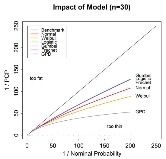
Figure 5.
Tail reliability diagram for maximum likelihood predictions for six two-parameter statistical models for a sample size of .
3.1.6. Impact of GPD Shape Parameter
We now consider the impact of the value of the shape parameter on the maximum likelihood reliability bias for the GPD, for a sample size of . Figure 6 shows that the reliability bias depends fairly strongly on the value of the shape parameter.
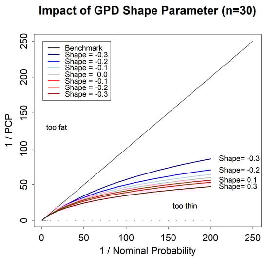
Figure 6.
Tail reliability diagram for maximum likelihood predictions for the generalized Pareto distribution (GPD) for different values of the shape parameter.
3.1.7. Impact of GEVD Shape Parameter
We now consider the impact of the value of the shape parameter on the maximum likelihood reliability bias for the GEVD for a sample size of . Figure 7 shows that the reliability bias depends only weakly on the value of the shape parameter.
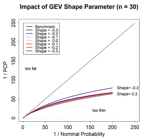
Figure 7.
Tail reliability diagram for maximum likelihood predictions for the generalized extreme value distribution (GEVD), for different values of the shape parameter.
3.1.8. Impact of Estimator: Normal Distribution
For the normal distribution, it is common to estimate parameters using the method of moments rather than maximum likelihood. We consider the version of method of moments in which the estimated variance is set to the standard unbiased estimator of the variance, which is different to, and larger than, the maximum likelihood estimate of the variance. Figure 8 compares the reliability bias for method of moments and maximum likelihood predictions for a sample size of . We see that the method of moments predictions have a slightly lower bias, which can be attributed to the larger variance. However, it is also clear that method of moments does not come close to eliminating the reliability bias. This is because it is still a point estimate method and ignores parameter uncertainty.
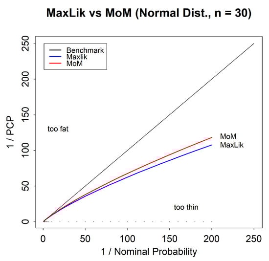
Figure 8.
Tail reliability diagram for predictions for the normal distribution for the method of moments and maximum likelihood predictions.
3.1.9. Impact of Estimator: GEVD
For the GEVD, it is common to use PWM to estimate the parameters, rather than maximum likelihood. Figure 9 compares the reliability bias for these two methods. We see that PWM gives a slightly lower reliability bias, but that the PWM bias is still large. Again, this is because it is still a point estimate method and ignores parameter uncertainty. For a detailed discussion of the differences between maximum likelihood and PWM fitting for the GEVD, see Coles and Dixon [16].
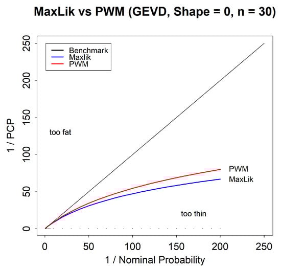
Figure 9.
Tail reliability diagram for predictions for the GEVD, for maximum likelihood and PWM predictions.
3.2. Point Estimate Prediction Reliability Bias Charts
We now describe the main output of this study, which are charts that illustrate the point estimate prediction reliability bias for 18 commonly used statistical models, as a function of sample size, NP and true parameter values. The models for which we have generated charts are listed in Appendix C, and the charts themselves are given in the Supplementary Materials. We show three kinds of charts, as follows.
3.2.1. Chart Type 1: PCP vs. NP and Sample Size
The first type of chart we show gives the inverse of the PCP as a function of the inverse NP and the sample size. For the homogeneous models, we only show a single chart that applies to all parameter values. For the inhomogeneous models we show multiple charts for different parameter values. An example is given in Figure 10, which illustrates this chart for the GEVD for a true shape parameter of . We discuss the usage of these charts and then interpret the results in Figure 10.
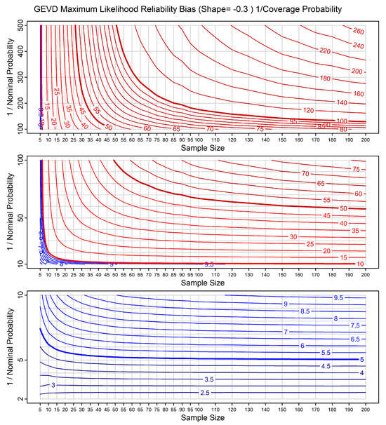
Figure 10.
Reliability bias chart for maximum likelihood predictions for data from the GEVD, with shape parameter . The horizontal axes show sample size and the vertical axes show inverse NP. The chart is divided into three sections in order to cover a range of inverse NPs, while maintaining scales that are linear in inverse NP, for easy comprehension. The contours show lines of constant inverse PCP. The colour and line thickness of the contour lines are varied to improve readability.
3.2.2. Chart Type 1: Usage
For all 18 models, we show results for maximum likelihood prediction. In addition, for the normal distribution we also show results for method of moments prediction. The horizontal axis in each chart is the sample size, and the vertical axis is the inverse NP. The variable shown by the contours is the inverse PCP. Each chart is split into three parts, covering different ranges of inverse NP. This allows us to use axes that are linear in inverse NP, are easy to read, give appropriate resolution in each range, and cover a wide range of probabilities, from to .
For the homogeneous models, the maximum likelihood charts can be used as follows:
- If a study with sample size n returns a maximum likelihood assessment of the probability of an event (or quantile) as being then we can use the appropriate chart to derive the PCP (i.e., the true probability) for that event, using the contours, as a function of n (on the horizontal axis) and (on the vertical axis). The PCPs are typically higher than the NPs. This is because the tail of maximum likelihood predictions is typically too thin.
- Alternatively, if we wish to find the event with PCP given by , from a maximum likelihood predictive distribution based on a sample size n, then we can read the corresponding NP, from the vertical axis. The event with PCP given by is the event with NP .
The method of moments results for the normal can be used in a corresponding way.
For the inhomogeneous models, the results can also be used in a similar way, with the caveat that they are only approximate, since they are given as a function of the true parameter value, which is unknown. In a real situation, one could estimate the true parameter value (perhaps using maximum likelihood) and use the chart or charts corresponding to the true parameter value or values closest to that estimate.
3.2.3. Chart Type 1: Interpretation
We note the following features in Figure 10: (a) in the lower right-hand corner of the figure, for large sample size and high NP (low inverse NP), the contours are close to horizontal, and the PCP agrees well with the NP. Parameter uncertainty is having little or no effect. For example, with a sample size of , events with an NP of have a PCP close to ; (b) in the top left-hand corner of the figure, for small sample size and low NP, the contours are close to vertical, and the NP and PCP are very different. Parameter uncertainty is having a large effect. For example, with a sample size of , events with an NP of have a PCP of between and , i.e., the events occur more than 25 times more frequently than predicted; (c) in between these two extremes, the lines are diagonal to varying degrees, illustrating varying impacts of parameter uncertainty. Climate studies often use a sample size of between and , corresponding to the availability of between 30 and 130 years of annual maximum data. For 30 data points, we see that the PCPs start to diverge from the NPs when the NP is less than . For 130 data points, they start to diverge when the NP is less than . This illustrates that having a larger sample size gives better results, but that even for what might be considered a relatively large sample size (), there is already material bias even for relatively high NPs; (d) for high NPs (bottom panel), parameter uncertainty is only material for the very smallest sample sizes; (e) for low NPs (top panel), parameter uncertainty is material for all sample sizes considered. The features in the type 1 charts for the other models are qualitatively the same as the features in Figure 10, although there may be large quantitative differences.
3.2.4. Chart Type 2: PCP vs NP and True Parameter
The second type of chart we show only applies to the GEVD and GPD models, including the GEVD with predictors. These models are inhomogeneous because of the shape parameter. This chart gives the inverse of the PCP as a function of the inverse of the NP and the shape parameter. We show different charts for different sample sizes. As an example, Figure 11 illustrates this chart for the GEVD for a sample size of . These charts can be used once the sample size is known.
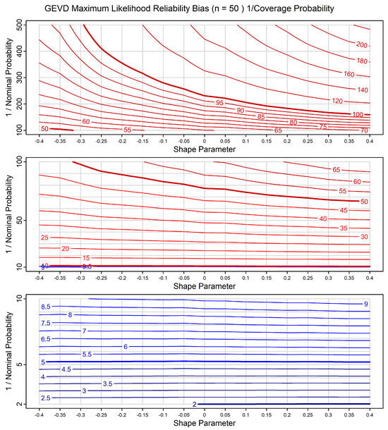
Figure 11.
Reliability bias chart for maximum likelihood predictions for data from the GEVD, for sample size of . The horizontal axes show true shape parameter and the vertical axes show inverse NP. As with Figure 10, the chart is divided into three sections in order to cover a range of inverse NPs, while maintaining scales that are linear in inverse NP, for easy comprehension. The contours show lines of constant inverse PCP. The colour and line thickness of the contour lines are varied to improve readability.
3.2.5. Chart Type 2: Interpretation
We note the following features in Figure 11: in the lower panel, the contours are close to horizontal. For NPs greater than , the reliability bias is relatively small. In the middle panel, we see moderate bias. For an NP of , the PCP varies from to as the shape parameter increases. In the top panel, we see large bias, especially for the lowest shape parameters. For an NP of , the PCP varies from to as the sample size increases.
3.2.6. Chart Type 3: Max. Exceedance vs True Parameter and Sample Size
The third type of chart we show only applies to the GEVD and GPD models, including the GEVD with predictors. The GEVD and GPD have a maximum value for the random variable when the shape parameter is negative. Both the true distribution, and a maximum likelihood fitted distribution, have these maxima. In roughly 50% of all cases, the maximum likelihood maximum will be below the true maximum, and, as a result, a sample from the true distribution may lie above the maximum likelihood maximum. These charts show the probability that a sample from the true distribution may lie above the maximum likelihood maximum.
Figure 12 illustrates this chart for the GEVD with 1 predictor. We see that for small sample sizes , a sample exceeds the predicted maximum with a probability of roughly 5%. For the large sample sizes , this probability decreases to roughly 0.1%. The probability also varies with the shape parameter, such that for more negative shape parameters the probability is larger.
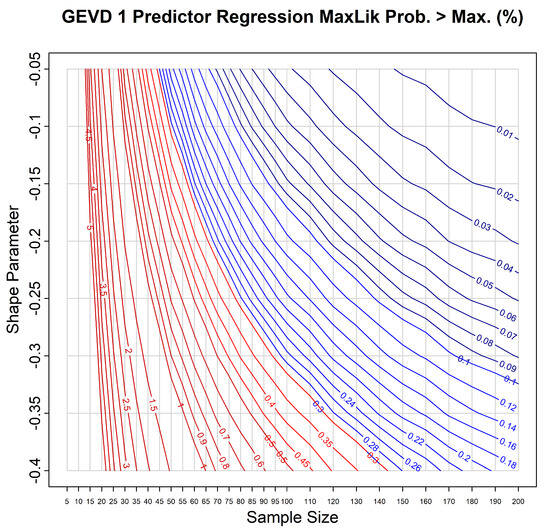
Figure 12.
Reliability bias chart for maximum likelihood predictions for data from the GEVD with a predictor on the location parameter, for sample size of . The horizontal axis shows sample size and the vertical axis shows shape parameter. The contours show lines of constant probability, for the probability that a single out-of-sample value will lie above the maximum likelihood estimate of the maximum value of the GEVD. Colour and line thickness of the contour lines are varied to improve readability.
3.3. Calibrating Prior Prediction Reliability Bias Charts
We also include calibrating prior prediction reliability bias charts for all 18 models. For 6 of the 18 models, we generate the predictions using analytic solutions (which we refer to as CP-Analytic predictions), and for the remaining 12 models, we generate the predictions using the DMGS quantile equation (which we refer to as CP-DMGS predictions).
3.3.1. Chart Type 1: PCP vs. NP and Sample Size
We include type 1 charts based on calibrating prior prediction for all the models listed in Appendix C. As an example, Figure 13 shows a type 1 calibrating prior prediction chart for the GEVD for a true shape parameter of , where the probabilities are generated using a calibrating prior and the DMGS quantile equation. We can compare this chart with the corresponding maximum likelihood results shown in Figure 10. We see that the calibrating prior results are also not exactly reliable. This is because the GEVD is not a homogeneous model and also because of the approximation involved in the DMGS equations. Considering Figure 13 in detail: for small sample sizes ( to ) and NPs of less than , the contours are steep, showing large differences between the NPs and the PCPs. However, as the sample size increases, the predictions now become more reliable much more rapidly than the maximum likelihood predictions shown in Figure 10. For example, for a sample size of , the maximum likelihood NP of corresponds to a quantile with a PCP of , while the calibrating prior NP of corresponds to a quantile with a PCP of between and .
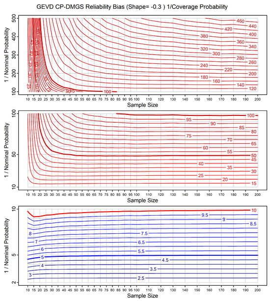
Figure 13.
As Figure 10 but now for calibrating prior predictions.
3.3.2. Chart Type 2: PCP vs. NP and True Parameter
We include type 2 charts for calibrating prior prediction for the GEVD and GPD models. As an example, Figure 14 shows a type 2 calibrating prior prediction chart for the GEVD for a sample size of . We can compare this chart with the corresponding maximum likelihood results shown in Figure 11. The calibrating prior predictions are materially more reliable. While the maximum likelihood results start to deviate from reasonable reliability for NPs of less than , the calibrating prior results only start to deviate from reasonable reliability for NPs of less than .
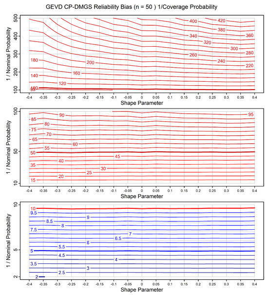
Figure 14.
As Figure 11 but now for calibrating prior predictions.
4. Discussion
We now discuss the results given above and in the Supplementary Materials.
Figure 1 shows that the standard reliability diagram is not adequate for evaluating reliability bias in the tail, but that there are various alternative versions of the reliability diagram, and in particular one that we call the tail reliability diagram, that can be used to identify reliability in the tail. This figure also shows that reliability bias is only material in the tail, but that in the tail it can be large, with PCP values five times or more larger than the NP.
In combination, the results of this study show that reliability bias depends strongly on the sample size, the number of parameters, the model, and the method used to generate predictions. For homogeneous models the reliability bias for the methods we have tested does not depend on the parameters of the model, but for inhomogeneous models it depends on any parameters that are not part of a transformation group. Even for what might be considered somewhat large sample sizes, such as , the maximum likelihood reliability bias may still be large enough that predictive probabilities are somewhat meaningless. For example, Figure 10 shows that for the GEV with a true shape parameter of , quantiles with an NP of have a PCP of .
Figure 4 shows that the dependence of maximum likelihood reliability bias on the number of parameters is large. It shows that for the GEV with and shape parameter of , and considering quantiles with an NP of , adding predictors to each parameter and thereby increasing the number of parameters from 3 to 6, increases the PCP from to .
Method of moments and PWM are sometimes used for the normal and GEVD, respectively, in an attempt to improve on maximum likelihood prediction. However, Figure 8 and Figure 9 show that the reliability bias improvement they give is more or less immaterial. This is because they also ignore parameter uncertainty. This suggests that other point estimate methods are likely to show equally little reduction in reliability bias.
For the GEVD and GPD, which are inhomogeneous, the precise value of the reliability bias cannot be determined because it depends on the true parameters, which are unknown. However, the dependence on the parameters is relatively weak, as we see in Figure 11. If the true parameter value can be estimated reasonably accurately, then our charts can give a good indication of the approximate magnitude of the reliability bias.
The calibrating prior prediction results show that reliability bias can be materially reduced using calibrating prior prediction. In some cases, when the model is homogeneous and the method for evaluating the prediction is based on exact closed-form expressions, the reliability bias is zero. In other cases, when the model is homogeneous but the method for evaluating the prediction is approximate, the reliability bias is small but non-zero. Finally, when the model is inhomogeneous, the reliability bias varies greatly as a function of sample size and nominal probability. For small sample sizes and extreme tail probabilities, it may be large. However, it is materially smaller than the reliability bias for maximum likelihood predictions, and for sample sizes and nominal probabilities similar to those used in scientific analyses, it is often small and may be sufficiently accurate.
5. Conclusions
Many scientific studies involve generating predictions of probabilities from continuous univariate parametric statistical models such as the normal distribution, simple linear regression, the GEVD, or the GEVD with predictors. Frequently, these predictions are generated by calculating point estimates of the parameters of the model and substituting those estimates into the model in place of the true unknown parameters. This approach neglects the uncertainty around the parameters and leads to a reliability bias in the resulting probabilities. The most notable feature of this reliability bias is that tail probabilities are typically underestimated compared to the relative frequencies of out-of-sample outcomes. Whether neglecting parameter uncertainty is a reasonable approximation or not depends on the tolerance to reliability bias, the model, the sample size and the part of the distribution that is of interest. The reliability bias typically increases as the number of parameters increases, as the sample size decreases, and as one considers predictions of more extreme events.
It is important to be able to assess the level of reliability bias involved in statistical prediction for two reasons. First, when evaluating the results from previous studies that have used point estimate prediction, one may wish to know whether the reliability bias has had a material impact on the results and their interpretation. Such an assessment may lead to the conclusion that the impact of reliability bias was sufficiently small that the results can be considered reasonable. However, the conclusion may be that the impact of the reliability bias was sufficiently large that the results need to be adjusted to correct for the bias, or recalculated using methods with lower reliability bias. Second, when designing new scientific studies, one may wish to assess whether point estimate prediction methods are suitable, given their reliability bias, or whether alternative methods with lower reliability bias should be used and how well they perform.
We have presented reliability bias charts based on maximum likelihood, method of moments, PWM and calibrating prior prediction, for 18 commonly used statistical models. These charts quantify reliability bias as a function of nominal probability (NP) and sample size and can be used to make both of the assessments described above. Because these charts consider multiple combinations of sample sizes and nominal probabilities, they contain orders of magnitude more information about predictive reliability bias than has previously been available. The charts show that maximum likelihood gives highly unreliable probabilities when using small sample sizes and when considering the extreme tail. For example, for a sample size of , for the GEVD with a shape parameter of , events with a maximum likelihood NP of have a predictive coverage probability (PCP) of only .
This reliability bias can be greatly reduced using objective Bayesian methods with calibrating priors, and we give a second set of charts, for the same 18 models, based on calibrating prior prediction. For some models, these methods give perfectly reliable predictions, for all sample sizes and all points in the tail. For other models, they do not give perfectly reliable predictions, but are still much more reliable than maximum likelihood. For example, for a sample size of , for the GEVD with shape parameter of , events with a calibrating prior prediction NP of have a PCP of between and . However, calibrating prior prediction still gives poor results for small sample sizes and the extreme tail. For these cases, future research may yield priors that give better results.
For more in-depth exploration and precise quantitative estimates of reliability bias, one can use the fitdistcp software, version 0.1.1. package that was used to generate the charts that we give [17]. For the evaluation of reliability bias for models that we have not covered in our analysis, it would be relatively straightforward to perform simulations of the type that we have performed. The author intends to maintain a website that gives the results from this study and also extends the results to other cases, at https://calibrationbias.info (accessed on 29 October 2025).
In summary, we recommend that great care should be taken when using probabilities calculated using point estimate methods such as maximum likelihood. In the tail, the probabilities may greatly underestimate the true probabilities. The size of the underestimation can be evaluated using the charts provided. It can also be compared with the reliability of probabilities generated using calibrating prior prediction, which can reduce the underestimation in most cases and eliminate it completely in some.
Supplementary Materials
The following supporting information can be downloaded at: https://www.mdpi.com/article/10.3390/stats8040109/s1.
Funding
The author is funded by a consortium of insurance companies to perform research into risk and uncertainty.
Institutional Review Board Statement
Not applicable.
Informed Consent Statement
Not applicable.
Data Availability Statement
No data were created during this study.
Acknowledgments
Many thanks to the insurance companies that support the author, to Trevor Sweeting, Lynne Jewson and the many others with whom I have discusssed this work, and to the three anonymous reviewers, whose comments greatly improved the manuscript.
Conflicts of Interest
The author’s research is funded by a group of insurance companies.
Appendix A. Abbreviations Used in This Study
| CDF | Cumulative distribution function | |
| CP | Calibrating prior | A prior chosen so that resulting predictions are reliable, a.k.a. well calibrated |
| CP-DMGS | Calibrating prior and DMGS | A specification of the prior and numerical scheme used to evaluate the Bayesian prediction equation |
| DMGS equations | Datta–Mukerjee–Ghosh–Sweeting | A set of equations that give approximate Bayesian predictions |
| EDF | Exceedance distribution function | One minus the CDF. Also known as the survival function. |
| GEV | Generalized extreme value | A distribution, used for maxima. |
| GEVD | Generalized extreme value distribution | |
| GP | Generalized Pareto | A distribution, used for tails |
| GPD | Generalized Pareto distribution | |
| NP | Nominal probability | The exceedance probability at which exceedance quantiles are to be calculated |
| PCP | Predictive coverage probability | The probability with which quantiles at a certain NP are exceeded |
| Probability density function | ||
| PWM | Probability weighted moments | A point estimate method for fitting distributions, often used for the GEVD |
| RHP | Right Haar prior | A prior with certain beneficial mathematical properties |
Appendix B. References to Studies Using Point Estimate Prediction
There are many hundreds of studies in the climate sciences that have used point estimate predictions to estimate extremes. A dozen recent examples are:
- Eden et al. [18] used the GEVD to analyze extreme precipitation.
- Gudmundsson and Seneviratne [19] used the Gamma distribution to analyze extreme precipitation.
- Kew et al. [20] used the normal distribution to model extreme soil moisture, and the GPD to model extreme precipitation.
- Otto et al. [21] used the GPD to model extreme temperatures.
- Philip et al. [22] used the normal to model extreme precipitation.
- Siswanto et al. [23] used the GEVD to model extreme precipitation.
- Stott et al. [24] used the GEVD to model extreme temperatures.
- van den Brink and Können [25] used the Gumbel to model extreme wind speeds.
- van der Wiel et al. [26] use the GEVD to model extreme precipitation.
- Vautard et al. [27] used the Gumbel to model precipitation.
- Thompson et al. [28] used the GEVD to model extreme temperature.
- Wehner et al. [29] used the GEVD to model extreme temperature and precipitation.
Appendix C. Details for the Statistical Models Considered
Appendix C.1. Exponential Distribution/Pareto Distribution with One Parameter
We use the exponential distribution with the exceedance distribution function (EDF) of the form
for parameter . If we apply the transformation for a constant then the EDF becomes
This is the EDF for a Pareto distribution with fixed scale parameter and shape parameter .
- The same charts apply to both models. Since both models are homogeneous, the results are independent of the parameter .
- Figure S1 shows the type 1 maximum likelihood reliability bias chart.
- Figure S83 shows the type 1 CP-Analytic reliability bias chart. Since both models are homogeneous, and we use an analytic solution, the CP-Analytic predictions are perfectly reliable and the contours are horizontal. The chart is only included for completeness.
Appendix C.2. Exponential Regression/Pareto Regression
We use the exponential distribution with 1 predictor t on the parameter, such that , giving the exceedance distribution function (EDF) of the form
for parameters . If we apply the transformation then the EDF becomes
This is the EDF for a Pareto distribution with fixed scale parameter and predictor t on the shape parameter.
- The same charts apply to both models. Since both models are homogeneous, the results are independent of the parameters.
- Figure S2 shows the type 1 maximum likelihood reliability bias chart.
- Figure S84 shows the type 1 CP-DMGS reliability bias chart. Since both models are homogeneous, the slight deviations from perfect reliability for small sample sizes and low probabilities are due to the approximation in the DMGS equations.
Appendix C.3. Normal Distribution/Log-Normal Distribution
We use the normal distribution with probability density function (PDF) of the form
for parameters . If we apply the transformation then the PDF becomes
This is the PDF for the log-normal distribution.
- The same charts apply to both models. Since both models are homogeneous, the results are independent of the parameters.
- Figure S3 shows the type 1 maximum likelihood reliability bias chart.
- Figure S85 shows the type 1 CP-Analytic reliability bias chart. Since both models are homogeneous, and we use an analytic solution, the predictions are perfectly reliable. The chart is only included for completeness.
Appendix C.4. Normal Distribution/Log-Normal Distribution, for Method of Moments
In the method of moments approach we use, we estimate the variance parameter using the standard unbiased expression:
where is the usual estimate for the mean.
- Figure S4 shows the type 1 method of moments reliability bias chart for the normal and log-normal distributions, but fitted with method of moments.
Appendix C.5. Gaussian Linear Regression with 1 Predictor/Log-Normal Regression with 1 Predictor
We use the normal distribution with a linear predictor t on the mean, i.e., simple linear regression, with probability density of the form
for parameters . If we apply the transformation then the PDF becomes
This is the PDF for log-normal regression.
- The same charts apply to both models. Since both models are homogeneous, the results are independent of the parameters.
- Figure S5 shows the type 1 maximum likelihood reliability bias chart.
- Figure S87 shows the type 1 CP-Analytic reliability bias chart. Since both models are homogeneous, and since we use an analytic solution, the predictions are perfectly reliable. The chart is only included for completeness.
Appendix C.6. Logistic Distribution
We use the logistic distribution with the cumulative distribution function (CDF) of the form
for parameters .
- Since this model is homogeneous, the results are independent of the parameters.
- Figure S6 shows the type 1 maximum likelihood reliability bias chart.
- Figure S88 shows the type 1 CP-DMGS reliability bias chart. Since this model is homogeneous, the slight deviations from perfect reliability for small sample sizes and low probabilities are due to the approximation in the DMGS equations.
Appendix C.7. Gumbel Distribution
We use the Gumbel distribution with the CDF of the form
for parameters .
- Since this model is homogeneous, the results are independent of the parameters.
- Figure S7 shows the type 1 maximum likelihood reliability bias chart.
- Figure S89 shows the type 1 CP-DMGS reliability bias chart for the Gumbel distribution. Since this model is homogeneous, the slight deviations from perfect reliability for small sample sizes and low probabilities are due to the approximation in the DMGS equations.
Appendix C.8. Gumbel Linear Regression
We use the Gumbel distribution with linear predictor t on the location parameter, with the CDF of the form
for parameters .
- Since this model is homogeneous, the results are independent of the parameters.
- Figure S8 shows the type 1 maximum likelihood reliability bias chart.
- Figure S90 shows the type 1 CP-DMGS reliability bias chart. Since this model is homogeneous, the slight deviations from perfect reliability for small sample sizes and low probabilities are due to the approximation in the DMGS equations.
Appendix C.9. Fréchet Distribution with Fixed Location Parameter
We use the Fréchet distribution with known location parameter , with the CDF of the form
for parameters .
- Since this model is homogeneous, the results are independent of the parameters.
- Figure S9 shows the type 1 maximum likelihood reliability bias chart.
- Figure S91 shows the type 1 CP-DMGS reliability bias chart. Since this model is homogeneous, the slight deviations from perfect reliability for small sample sizes and low probabilities are due to the approximation in the DMGS equations.
Appendix C.10. Weibull Distribution
We use the Weibull distribution with the EDF of the form
for parameters .
- Since this model is homogeneous, the results are independent of the parameters.
- Figure S10 shows the type 1 maximum likelihood reliability bias chart.
- Figure S92 shows the type 1 CP-DMGS reliability bias chart. Since this model is homogeneous, the slight deviations from perfect reliability for small sample sizes and low probabilities are due to the approximation in the DMGS equations.
Appendix C.11. Generalized Extreme Value Distribution
We use the GEVD with the CDF of the form
where
for parameters .
- Since this model is inhomogeneous, the results depend on the shape parameter .
- Type 1 charts for maximum likelihood prediction are shown in Figures S11 to S19 for values of the shape parameter from to .
- Type 2 charts for maximum likelihood prediction are shown in Figures S47 to S54 for sample sizes from to .
- A type 3 chart for maximum likelihood prediction is shown in Figure S79.
- The calibrating prior GEVD results are based on predictions generated using a prior of . This prior is recommended as a calibrating prior by Jewson et al. [11].
- Type 1 CP-DMGS reliability bias charts are shown in Figures S93 to S101 for values of the shape parameter from to .
- Type 2 CP-DMGS charts are shown in Figures S129 to S136 for sample sizes from to .
- Type 3 charts are not relevant for Bayesian predictions, as there is no upper limit to the random variable in the predictions.
Appendix C.12. Generalized Extreme Value 1 Predictor Regression
We use the GEVD with one predictor u with the CDF of the form
where
for parameters .
- Since this model is inhomogeneous, the results depend on the shape parameter .
- Type 1 charts for maximum likelihood prediction are shown in Figures S20 to S28 for values of the shape parameter from to .
- Type 2 charts for maximum likelihood prediction are shown in Figures S55 to S62 for sample sizes from to .
- A type 3 chart for maximum likelihood prediction is shown in Figure S80.
- The calibrating prior GEVD-with-1-predictor results are based on predictions generated using a prior of . This prior is recommended as a calibrating prior by Jewson et al. [11].
- Type 1 CP-DMGS reliability bias charts are shown in Figures S102 to S110 for values of the shape parameter from to .
- Type 2 CP-DMGS charts are shown in Figures S137 to S144 for sample sizes from to .
Appendix C.13. Generalized Extreme Value 2 Predictor Regression
We use the GEVD with two predictors with the CDF of the form
where
for parameters .
- Since this model is inhomogeneous, the results depend on the shape parameter .
- Type 1 charts for maximum likelihood prediction are shown in Figures S29 to S37 for values of the shape parameter from to .
- Type 2 charts for maximum likelihood prediction are shown in Figures S63 to S70 for sample sizes from to .
- A type 3 chart for maximum likelihood prediction is shown in Figure S81.
- The calibrating prior GEVD-with-2-predictors results are based on predictions generated using a prior of . This prior is recommended as a calibrating prior by Jewson et al. [11].
- Type 1 CP-DMGS reliability bias charts are shown in Figures S111 to S119 for values of the shape parameter from to .
- Type 2 CP-DMGS reliability bias charts are shown in Figures S145 to S152 for sample sizes from to .
Appendix C.14. Generalized Pareto Distribution
We use the GPD with the EDF of the form
for parameters .
- Since this model is inhomogeneous, the results depend on the shape parameter .
- Type 1 charts for maximum likelihood prediction are shown in Figures S38 to S46 for values of the shape parameter from to .
- Type 2 charts for maximum likelihood prediction are shown in Figures S71 to S78 for sample sizes from to .
- A type 3 chart for maximum likelihood prediction is shown in Figure S82.
- The calibrating prior GPD results are based on predictions generated using a prior of . This prior is recommended as a calibrating prior by Jewson et al. [11].
- Type 1 CP-DMGS reliability bias charts are shown in Figures S120 to S128 for values of the shape parameter from to .
- Type 2 CP-DMGS charts are shown in Figures S153 to S160 for sample sizes from to .
References
- Priestley, M.D.K.; Stephenson, D.B.; Scaife, A.A.; Bannister, D.; Allen, C.J.T.; Wilkie, D. Return levels of extreme European windstorms, their dependency on the North Atlantic Oscillation, and potential future risks. Nat. Hazards Earth Syst. Sci. 2023, 23, 3845–3861. [Google Scholar] [CrossRef]
- Barnes, C.; Jain, P.; Keeping, T.R.; Gillett, N.; Boucher, J.; Gachon, P.; Heinrich, D.; Kirchmeier-Young, M.; Boulanger, Y. Disentangling the roles of natural variability and climate change in Canada’s 2023 fire season. Environ. Res. Clim. 2025, 4, 035013. [Google Scholar] [CrossRef]
- Cho, E.; Ahmadisharaf, E.; Villarini, G.; AghaKouchak, A. Historical changes in overtopping probability of dams in the United States. Nat. Commun. 2025, 16, 6693. [Google Scholar] [CrossRef]
- Quilcaille, Y.; Gudmundsson, L.; Schumacher, D.L.; Gasser, T.; Heede, R.; Heri, C.; Lejeune, Q.; Nath, S.; Naveau, P.; Thiery, W.; et al. Systematic attribution of heatwaves to the emissions of carbon majors. Nature 2025, 645, 392–398. [Google Scholar] [CrossRef] [PubMed]
- Bernardo, J.; Smith, A. Bayesian Theory; Wiley: Hoboken, NJ, USA, 1993. [Google Scholar]
- Geisser, S. Predictive Inference: An Introduction; Chapman and Hall: New York, NY, USA, 1993. [Google Scholar]
- Root, H.E. Probability Statements in Weather Forecasting. J. Appl. Meteorol. Climatol. 1962, 1, 163–168. [Google Scholar] [CrossRef][Green Version]
- Niculescu-Mizil, A.; Caruana, R. Predicting good probabilities with supervised learning. In Proceedings of the 22nd International Conference on Machine Learning, ICML ’05, Bonn, Germany, 7–11 August 2005; Association for Computing Machinery: New York, NY, USA, 2005; pp. 625–632. [Google Scholar] [CrossRef]
- Gerrard, R.; Tsanakas, A. Failure Probability Under Parameter Uncertainty. Risk Anal. 2011, 31, 727–744. [Google Scholar] [CrossRef] [PubMed]
- Blanco, D.; Weng, A. Practical aspects of modelling parameter uncertainty for risk capital calculation. Z. Für Die Gesamte Versicherungswissenschaft 2019, 108, 43–62. [Google Scholar] [CrossRef]
- Jewson, S.; Sweeting, T.; Jewson, L. Reducing reliability bias in assessments of extreme weather risk using calibrating priors. ASCMO 2025, 11, 1–22. [Google Scholar] [CrossRef]
- Severini, T.; Mukerjee, R.; Ghosh, M. On an exact probability matching property of right-invariant priors. Biometrika 2002, 89, 952–957. [Google Scholar] [CrossRef]
- Fraser, D. The Fiducial Method and Invariance. Biometrika 1961, 48, 261–280. [Google Scholar] [CrossRef]
- Hora, R.B.; Buehler, R.J. Fiducial Theory and Invariant Estimation. Ann. Math. Stat. 1966, 37, 643–656. [Google Scholar] [CrossRef]
- Datta, G.; Mukerjee, R.; Ghosh, M.; Sweeting, T. Bayesian prediction with approximate frequentist validity. Ann. Stat. 2000, 28, 1414–1426. [Google Scholar] [CrossRef]
- Coles, S.G.; Dixon, M.J. Likelihood-Based Inference for Extreme Value Models. Extremes 1999, 2, 5–23. [Google Scholar] [CrossRef]
- Jewson, S. Fitdistcp, R package version 0.1.1; 2025. Available online: https://cran.r-project.org/web/packages/fitdistcp/index.html (accessed on 29 October 2025).
- Eden, J.M.; Kew, S.F.; Bellprat, O.; Lenderink, G.; Manola, I.; Omrani, H.; van Oldenborgh, G.J. Extreme precipitation in the Netherlands: An event attribution case study. Weather Clim. Extrem. 2018, 21, 90–101. [Google Scholar] [CrossRef]
- Gudmundsson, L.; Seneviratne, S.I. Anthropogenic climate change affects meteorological drought risk in Europe. Environ. Res. Lett. 2016, 11, 044005. [Google Scholar] [CrossRef]
- Kew, S.; Philip, S.; van Oldenborgh, G.J.; van der Schrier, G.; Otto, F.E.L.; Vautard, R. The Exceptional Summer Heat Wave in Southern Europe 2017. Bull. Am. Meteorol. Soc. 2019, 100, S49–S53. [Google Scholar] [CrossRef]
- Otto, F.E.L.; Massey, N.; van Oldenborgh, G.J.; Jones, R.G.; Allen, M.R. Reconciling two approaches to attribution of the 2010 Russian heat wave. Geophys. Res. Lett. 2012, 39, L04702. [Google Scholar] [CrossRef]
- Philip, S.; Kew, S.F.; van Oldenborgh, G.J.; Otto, F.; O’Keefe, S.; Haustein, K.; King, A.; Zegeye, A.; Eshetu, Z.; Hailemariam, K.; et al. Attribution Analysis of the Ethiopian Drought of 2015. J. Clim. 2018, 31, 2465–2486. [Google Scholar] [CrossRef]
- Siswanto; van Oldenborgh, G.J.; van der Schrier, G.; Lenderink, G.; van den Hurk, B. Trends in High-Daily Precipitation Events in Jakarta and the Flooding of January 2014. Bull. Am. Meteorol. Soc. 2015, 96, S131–S135. [Google Scholar] [CrossRef]
- Stott, P.A.; Christidis, N.; Otto, F.E.L.; Sun, Y.; Vanderlinden, J.P.; van Oldenborgh, G.J.; Vautard, R.; von Storch, H.; Walton, P.; Yiou, P.; et al. Attribution of extreme weather and climate-related events. WIREs Clim. Chang. 2016, 7, 23–41. [Google Scholar] [CrossRef]
- van den Brink, H.W.; Können, G.P. Estimating 10000-year return values from short time series. Int. J. Climatol. 2011, 31, 115–126. [Google Scholar] [CrossRef]
- van der Wiel, K.; Kapnick, S.B.; van Oldenborgh, G.J.; Whan, K.; Philip, S.; Vecchi, G.A.; Singh, R.K.; Arrighi, J.; Cullen, H. Rapid attribution of the August 2016 flood-inducing extreme precipitation in south Louisiana to climate change. Hydrol. Earth Syst. Sci. 2017, 21, 897–921. [Google Scholar] [CrossRef]
- Vautard, R.; Yiou, P.; van Oldenborgh, G.J.; Lenderink, G.; Thao, S.; Ribes, A.; Planton, S.; Dubuisson, B.; Soubeyroux, J.M. Extreme Fall 2014 Precipitation in the Cévennes Mountains. Bull. Am. Meteorol. Soc. 2015, 96, S56–S60. [Google Scholar] [CrossRef]
- Thompson, V.; Mitchell, D.; Hegerl, G.; Collins, M.; Leach, N.; Slingo, J. The most at-risk regions in the world for high-impact heatwaves. Nat. Commun. 2023, 14, 2152. [Google Scholar] [CrossRef] [PubMed]
- Wehner, M.; Gleckler, P.; Lee, J. Characterization of long period return values of extreme daily temperature and precipitation in the CMIP6 models: Part 1, model evaluation. Weather Clim. Extrem. 2020, 30, 100283. [Google Scholar] [CrossRef]
Disclaimer/Publisher’s Note: The statements, opinions and data contained in all publications are solely those of the individual author(s) and contributor(s) and not of MDPI and/or the editor(s). MDPI and/or the editor(s) disclaim responsibility for any injury to people or property resulting from any ideas, methods, instructions or products referred to in the content. |
© 2025 by the author. Licensee MDPI, Basel, Switzerland. This article is an open access article distributed under the terms and conditions of the Creative Commons Attribution (CC BY) license (https://creativecommons.org/licenses/by/4.0/).