Probabilistic Links Between Quantum Classification of Patterns of Boolean Functions and Hamming Distance

Abstract

This article investigates the probabilistic relationship between quantum classification of Boolean functions and their Hamming distance. By integrating concepts from quantum computing, information theory, and combinatorics, we explore how Hamming distance serves as a metric for analyzing deviations in function classification. Our extensive experimental results confirm that the Hamming distance is a pivotal metric for validating nearest neighbors in the process of classifying random functions. One of the significant conclusions we arrived is that the successful classification probability decreases monotonically with the Hamming distance. However, key exceptions were found in specific classes, revealing intra-class heterogeneity. We have established that these deviations are not random but are systemic and predictable. Furthermore, we were able to quantify these irregularities, turning potential errors into manageable phenomena. The most important novelty of this work is the demarcation, for the first time to the best of our knowledge, of precise Hamming distance intervals for the classification probability. These intervals bound the possible values the probability can assume, and provide a new foundational tool for probabilistic assessment in quantum classification. Practitioners can now endorse classification results with high certainty or dismiss them with confidence. This framework can significantly enhance any quantum classification algorithm’s reliability and decision-making capability.

1. Introduction

Today Quantum computing is advancing rapidly, with recent breakthroughs suggesting that transformative quantum systems may soon emerge, even though current quantum computers are not yet capable of fully disrupting classical paradigms. Major industry players have made significant strides. IBM introduced the 1121-qubit Condor and high-performance R2 Heron, building on the 127-qubit Eagle [1] and 433-qubit Osprey [2,3,4]. Google demonstrated quantum computers outperforming advanced supercomputers [5,6]. Microsoft unveiled the Majorana 1 quantum chip [7,8,9] D-Wave’s quantum annealer solved a scientifically significant problem faster than classical computers [10,11]. China’s 105-qubit Zuchongzhi 3.0 processor marked a technological milestone [12,13]. Other innovations include novel design concepts [14,15], hardware advancements [16,17], and distributed quantum computing, where two processors were linked via a photonic network to function as a single system [18,19]. These developments underscore the growing feasibility of distributed quantum systems and their potential for applications like quantum classification of Boolean functions.

This study explores quantum classification of Boolean functions from a novel perspective, focusing on probabilistic correlations with Hamming distance. Quantum algorithms can perfectly classify functions with specific properties (probability 1), but our goal is to understand classification behavior when functions deviate from these properties, using Hamming distance as a metric. The Deutsch-Jozsa algorithm [20] pioneered this field, followed by extensions such as multidimensional variants [21], analyses of balanced functions [22,23], and generalizations [24,25,26]. Practical applications [27,28] and distributed versions [29,30] further advanced the field, while [31] extended Deutsch’s algorithm to binary Boolean functions. Quantum learning literature often focuses on distinguishing constant and balanced functions [32,33,34,35,36,37], but a recent study [38] targets imbalanced functions, proposing the Boolean Function Pattern Quantum Classifier (BFPQC) for classifying functions with specific behavioral patterns.

We present our exposition as a quantum game featuring Alice and Bob, using the engaging nature of games to clarify complex concepts. Quantum games, popularized since 1999 [39,40], often outperform classical strategies [41], as exemplified by the Prisoners’ Dilemma [40] and other abstract games [42]. Beyond entertainment, quantum games have addressed serious problems like cryptographic protocols [43,44,45]. Our game-based framework makes the probabilistic links between quantum classification and Hamming distance more accessible, offering a novel tool for advancing quantum algorithm design.

Contribution. This work capitalizes upon recent prior studies, such as [38,46], to investigate the usefulness of the Hamming distance as metric between Boolean functions, that can yield meaningful insights when the quantum classification algorithm encounters an unknown function outside its scope. This is a challenging benchmark that stresses the robustness and versatility limits of any quantum classification algorithm. The main strengths of this work are summarized below.

• Our extensive experimental results robustly validate the Hamming distance as a critical and effective metric for verifying or disqualifying potential nearest neighbor candidates in the classification process.
• As anticipated, we confirm that the classification threshold is a monotonically decreasing function of the Hamming distance. This foundational trend, however, is punctuated by the notable exceptions identified for specific classes in Section 5.4. These exceptions are not mere statistical artifacts; they provide crucial insight into intra-class heterogeneity, demonstrating how individual functions can cause significant deviations from the global behavioral pattern.
• Crucially, our analysis reveals that even these deviations are systemic. The irregularities observed in special classes are not random but can be rigorously quantified and predicted. This transforms a potential source of error into a manageable, well-understood aspect of the classification landscape.
• To the best of our knowledge, this work is the first to establish precise intervals for Hamming distances that bound the possible values of the classification threshold. By quantifying this relationship, we provide a foundational tool for probabilistic reasoning within quantum classification paradigms.
• This capability is of paramount practical importance. It equips practitioners with a powerful framework to either:
  • confidently endorse a classification result with high certainty when it is likely a true nearest neighbor, or
  • decisively dismiss a result when the probability of it being a genuine nearest neighbor is vanishingly small.
  This directly enhances the reliability and efficiency of the classification system.

Organization

This article is structured in the following way. Section 1 introduces the topic and provides references to relevant literature. Section 2 contains a brief overview of key concepts and technical details. Section 3 defined the notion of perfectly classifiable Boolean function, while the following Section 4 introduces the theoretical machinery that establishes the framework for classifying functions outside of the promised class. Section 5 presents and analyzes the entire suite of experiments we have undertaken in this work. Finally, the paper wraps up with a summary and a discussion of the Nearest Basis Ket Game in Section 6.

2. Preliminary Concepts

This section introduces the notation and terminology that will be used throughout this work.

• $\mathbb{B}$ denotes the binary set $\{0,1\}$.
• A bit vector $\mathbf{b}$ is a sequence of n bits: $b_{n-1}\dots b_0$. For succinctness it is helpful to consider it as an element of ${\mathbb{B}}^n$ and write $\mathbf{b}\in {\mathbb{B}}^n$. The special bit vectors $\mathbf{0}=0\dots 0$ and $\mathbf{1}=1\dots 1$ represent vectors with all bits set to zero and one, respectively.
• Bit vectors $\mathbf{b}\in {\mathbb{B}}^n$ are written in boldface to distinguish them from scalar quantities. Throughout this work, $\mathbf{b}$ will also be interpreted as the binary representation of an integer b.
• Each bit vector $\mathbf{b}\in {\mathbb{B}}^n$ corresponds to one of the $2^n$ basis kets forming the computational basis of a $2^n$-dimensional Hilbert space.

The Hamming distance is a metric used to quantify the difference between two strings of equal length over a fixed alphabet. In our setting, which involves bit vectors, if we are given two bit vectors $\mathbf{a},\mathbf{b}\in {\mathbb{B}}^n$, their Hamming distance $d_H(\mathbf{a},\mathbf{b})$ is defined as the number of positions at which the corresponding bits differ.

Definition 1

(Hamming Distance). Let $\mathbf{a}=a_{n-1}\dots a_0$ and $\mathbf{b}=b_{n-1}\dots b_0$ be two binary strings in ${\mathbb{B}}^n$, $n\ge 1$. Their Hamming distance, denoted by $d_H(\mathbf{a},\mathbf{b})$, is given by:

$$\begin{array}{c}\hfill d_H(\mathbf{a},\mathbf{b})≔\sum _{i=0}^{n-1}{a}_i\oplus b_i,\hfill \end{array}$$

(1)

where ⊕ stands for the XOR operation, since $a_i\oplus b_i=1$ if and only if $a_i\ne b_i$.

Oracles are a cornerstone of quantum computing, acting as black-box components in many quantum algorithms. They encapsulate a function or specific information within a quantum circuit, enabling efficient problem-solving compared to classical methods in certain cases. Oracles evaluate a function or verify conditions without revealing their internal workings, often providing insights into a function’s properties or identifying solutions. For this article, we adopt the following definition.

Definition 2

(Oracle & Unitary Transform). An oracle is a black box that implements a Boolean function f. As a black box, its internal mechanics are opaque, but it is assumed to operate correctly. The oracle enables the construction of a unitary transform $U_f$ that encodes the behavior of f according to the standard schema:

$$\begin{array}{c}\hfill U_f:|y\rangle |\mathbf{x}\rangle \to |y\oplus f(\mathbf{x})\rangle |\mathbf{x}\rangle .\hfill \end{array}$$

(2)

In this work, we assume all oracles and their unitary transforms follow Equation (2) and are used to infer properties of a function based on its behavior.

For completeness, we define the following states |+〉 and |−〉:

$$\begin{array}{c}\hfill |+\rangle =H|0\rangle ={\displaystyle \frac{|0\rangle +|1\rangle }{\sqrt{2}}}\hfill \end{array}$$

(3)

$$\begin{array}{c}\hfill |-\rangle =H|1\rangle ={\displaystyle \frac{|0\rangle -|1\rangle }{\sqrt{2}}}\hfill \end{array}$$

(4)

To extract useful information from the schema in Equation (2), we set $|y\rangle =|-\rangle$, yielding the following form:

$$\begin{array}{c}\hfill U_f:|-\rangle |\mathbf{x}\rangle \to {(-1)}^{f\left(\mathbf{x}\right)}|-\rangle |\mathbf{x}\rangle .\hfill \end{array}$$

(5)

We frequently refer to the following state, termed the perfect superposition state:

$$\begin{array}{cc}\hfill |\phi \rangle \hfill & \hfill =2^{-{\displaystyle \frac{n}{2}}}\sum _{\mathbf{x}\in {\mathbb{B}}^n}|\mathbf{x}\rangle ,\hfill \end{array}$$

(6)

which serves as the standard starting point for most quantum algorithms. It is typically generated by applying the n-fold Hadamard transform to the initial state ${|0\rangle }^{\otimes n}$.

Bitwise addition modulo 2 extends the XOR operation to bit vectors, providing a natural generalization.

Definition 3

(Bitwise Addition Modulo 2). For two bit vectors $\mathbf{x},\mathbf{y}\in {\mathbb{B}}^n$, with $\mathbf{x}=x_{n-1}\dots x_0$ and $\mathbf{y}=y_{n-1}\dots y_0$, their bitwise sum modulo 2, denoted by $\mathbf{x}\oplus \mathbf{y}$, is defined as:

$$\mathbf{x}\oplus \mathbf{y}≔(x_{n-1}\oplus y_{n-1})\dots (x_0\oplus y_0).$$

(7)

We use the symbol ⊕ for both single-bit addition modulo 2 and bitwise addition modulo 2, as the context clarifies the intended operation.

3. Perfectly Classifiable Boolean Functions

Quantum Boolean classification algorithms typically enable the classification of Boolean functions that satisfy specific properties with a probability of 1. In the literature, these functions are often described as satisfying a “promise,” meaning they are guaranteed to possess certain characteristics, giving rise to the term “promise problem.” For example, in the quantum classification algorithm introduced in [38], the promise is that the behavior of the classifiable Boolean functions expresses “imbalance” in the number of zero and one values they assume.

To facilitate the analysis of Boolean functions and their classification, we shall introduce the concept of pattern bit vectors, which provide a compact and computationally convenient representation of Boolean functions. This abstraction enables the use of the Hamming distance between two pattern bit vectors as a measure of the dissimilarity between their corresponding Boolean functions.

Definition 4

(Pattern Bit Vector). Let $f:{\mathbb{B}}^n\to \mathbb{B}$, $n\ge 1$, be a Boolean function. We define the pattern bit vector of f as a unique bit vector that encodes the function’s output values across all possible inputs. The formal construction is as follows:

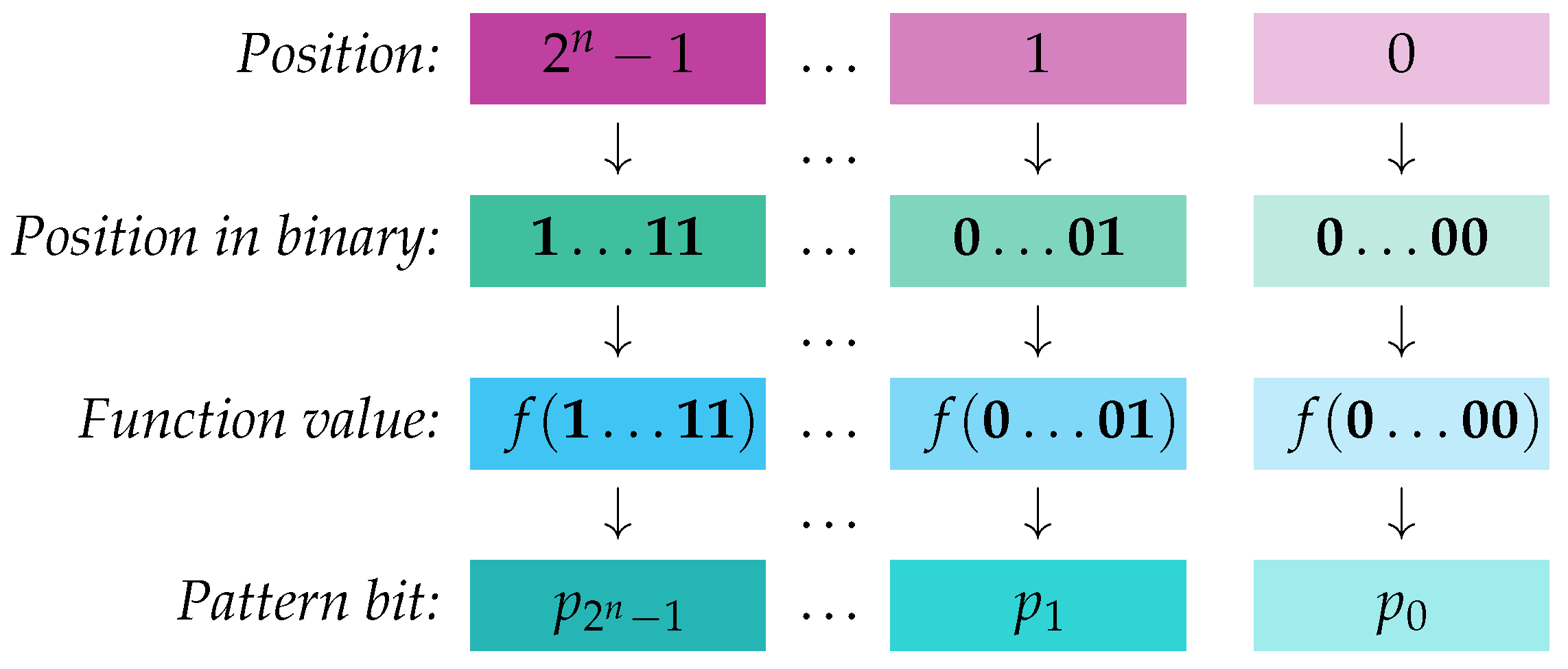
• The pattern bit vector ${\mathbf{p}}_f=p_{2^n-1}\dots p_1{p}_0\in {\mathbb{B}}^{2^n}$ is defined such that $p_i=f\left(\mathbf{i}\right)$, where $\mathbf{i}\in {\mathbb{B}}^n$ is the binary bit vector representing the integer i, for $0\le i\le 2^n-1$. Thus, ${\mathbf{p}}_f$ systematically records the values of $f\left(\mathbf{i}\right)$ as $\mathbf{i}$ ranges over all possible inputs in ${\mathbb{B}}^n$, as depicted in Figure 1.
• The negation of the pattern bit vector, denoted $\overline{{\mathbf{p}}_f}=\overline{p_{2^n-1}}\dots \overline{p_1}\overline{p_0}$, is the pattern bit vector corresponding to the negated function $\overline{f}$, where $\overline{f}\left(\mathbf{i}\right)=\neg f\left(\mathbf{i}\right)$ for all $\mathbf{i}\in {\mathbb{B}}^n$.

Definition 5

(Function Realizing Pattern Vector). Conversely, given any pattern bit vector $\mathbf{p}$ = $p_{2^n-1}$…$p_1$$p_0$∈${\mathbb{B}}^{2^n}$, we define the Boolean function $f_{\mathbf{p}}:{\mathbb{B}}^n\to \mathbb{B}$ such that $f_{\mathbf{p}}\left(\mathbf{i}\right)=p_i$, where $\mathbf{i}\in {\mathbb{B}}^n$ is the binary bit vector representing the integer i, for $0\le i\le 2^n-1$. This establishes a unique Boolean function $f_{\mathbf{p}}$ associated with the pattern bit vector $\mathbf{p}$, termed the realization of $\mathbf{p}$.

The preceding definitions establish a bijective correspondence between Boolean functions $f:{\mathbb{B}}^n\to \mathbb{B}$ and their pattern bit vectors in ${\mathbb{B}}^{2^n}$. In essence, a Boolean function and its pattern bit vector are two representations of the same mathematical object, akin to dual perspectives of a single entity. Knowing the behavior of a Boolean function allows the construction of its pattern bit vector, while the pattern bit vector fully encodes the information required to reconstruct the function. This duality is particularly advantageous, as it enables simple and efficient manipulation of functions via their bit vector representations.

Example 1

(Functions & Patterns). For example, consider a Boolean function $f:{\mathbb{B}}^2\to \mathbb{B}$ defined by $f\left(00\right)=0$, $f\left(01\right)=1$, $f\left(10\right)=0$, and $f\left(11\right)=1$. Its pattern bit vector is ${\mathbf{p}}_f=p_3{p}_2{p}_1{p}_0=f\left(11\right)f\left(10\right)f\left(01\right)f\left(00\right)=1010$. Conversely, given the pattern bit vector ${\mathbf{p}}_f=1010$, we can reconstruct the function $f_{\mathbf{p}}$ with the same input-output mappings. This equivalence highlights the one-to-one correspondence between Boolean functions and their pattern bit vectors. The concept of pattern bit vector provides a succinct way to represent the behavior of more complex Boolean functions, such as function $g:{\mathbb{B}}^4\to \mathbb{B}$, which takes the values shown in

Table 1. Truth values of the function $g:{\mathbb{B}}^4\to \mathbb{B}$.

	0000	0001	0010	0011	0100	0101	0110	0111	1000	1001	1010	1011	1100	1101	1110	1111
g	0	1	1	1	1	0	0	0	1	0	0	0	0	0	0	0

and is described by the pattern vector ${\mathbf{p}}_g=0000000100011110$.

Definition 6

(Pattern Basis). A pattern basis of rank n, $n\ge 1$, denoted by $P_n$, is a list of $2^n$ pattern bit vectors $({\mathbf{p}}_0,{\mathbf{p}}_1,\dots ,{\mathbf{p}}_{2^n-1})$, each of length $2^n$, that satisfy the pairwise orthogonality property:

$$\begin{array}{c}\hfill {\mathbf{p}}_i\oplus {\mathbf{p}}_j\mathit{contains}{2}^{n-1}0s\mathit{and}{2}^{n-1}1s,0\le i\ne j\le n-1.\hfill \end{array}$$

(8)

Example 2

(Pattern Bases). Let $B_1$ and $Q_2$ be the following lists of pattern vectors:

$$B_1≔({\mathbf{e}}_0=00,{\mathbf{e}}_1=01),\hspace{1em}\hspace{1em}\mathit{and}$$

(9)

$$Q_2≔({\mathbf{g}}_0=0001,{\mathbf{g}}_1=0010,{\mathbf{g}}_2=0100,{\mathbf{g}}_3=1000).$$

(10)

Every ${\mathbf{e}}_i$ has length $2^1=2$ and is orthogonal to every other ${\mathbf{e}}_j$, $i\ne j$, and, similarly, every ${\mathbf{g}}_i$ has length $2^2=4$ and is orthogonal to every other ${\mathbf{g}}_j$, $i\ne j$. Furthermore, $B_1$ consists of $2^1=2$ pattern bit vectors and $Q_2$ consists of $2^2=4$ pattern bit vectors. Therefore, by Definition 6, $B_1$ and $Q_2$ are two pattern bases of rank 1 and 2, respectively.

Definition 7

(Function Class Realizing Pattern Basis). Let $P_n$ = $({\mathbf{p}}_0,{\mathbf{p}}_1,$ …$,{\mathbf{p}}_{2^n-1})$ be a pattern basis of rank n. To $P_n$ we associate the class $F_{P_n}$ = $(f_{{\mathbf{p}}_0},f_{{\mathbf{p}}_1},$ …$,f_{{\mathbf{p}}_{2^n-1}})$ of Boolean functions from ${\mathbb{B}}^n$ to $\mathbb{B}$ such that $f_{{\mathbf{p}}_i}$, $0\le i\le 2^n-1$, is the function realizing the pattern bit vector ${\mathbf{p}}_i$. We say that the class of Boolean functions $F_{P_n}$ realizes the pattern basis $P_n$.

Definition 8

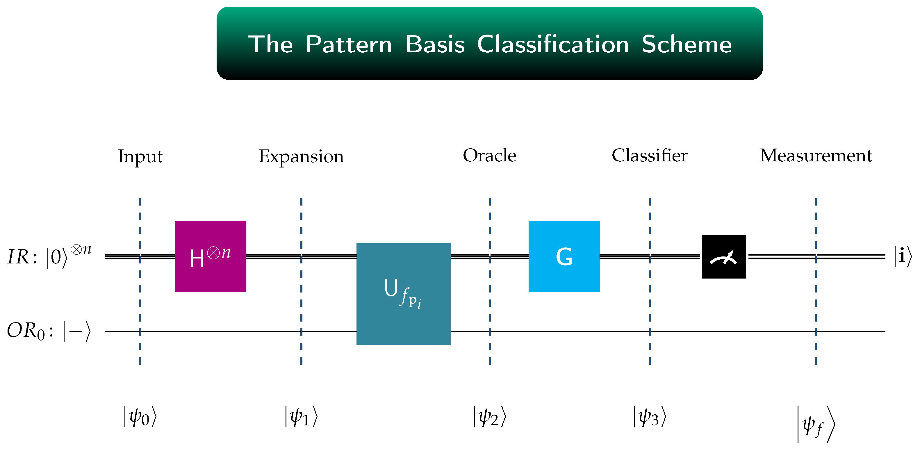
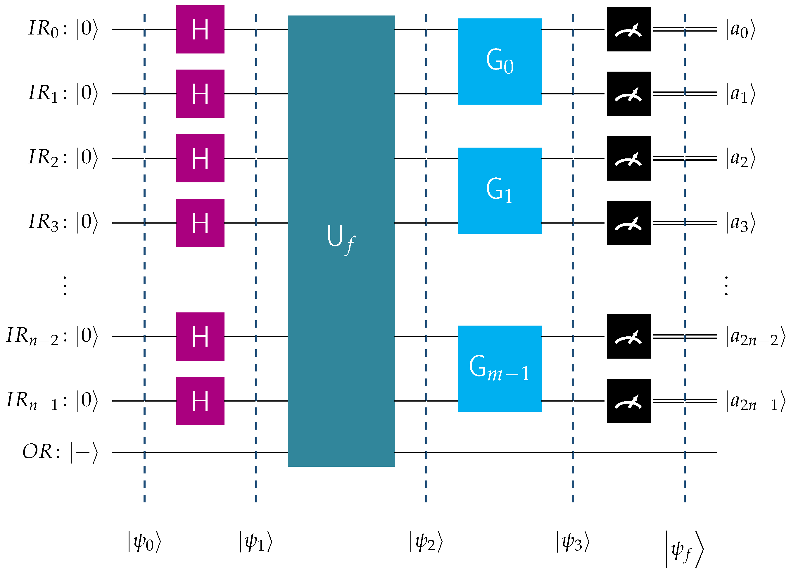
(The Pattern Basis Classification Scheme). Let $P_n$ be a pattern basis of rank n and let $F_{P_n}$ be the class of Boolean functions realizing $P_n$. We say that $P_n$ admits a classification scheme, if there exists an abstract quantum circuit, such as the one depicted in Figure 2, satisfying the pattern basis classification property. This property asserts that if $U_{f_{{\mathbf{p}}_i}}$ is an oracle for the function $f_{{\mathbf{p}}_i}\in F_{P_n}$ that realizes the pattern bit vector ${\mathbf{p}}_i\in P_n$, then, with probability 1, the outcome of the final measurement is the basis ket $|\mathbf{i}\rangle$, $\mathbf{i}$ being the binary representation of the index i.

We clarify the symbolism employed in Figure 2:

• $IR$ denotes the quantum input register, containing n qubits.
• $OR$ is the single-qubit output register, initialized to |−〉.
• $U_{f_{{\mathbf{p}}_i}}$ designates the unitary transform that implements the oracle for the function $f_{{\mathbf{p}}_i}$. Its exact form depends on $f_{{\mathbf{p}}_i}$ and satisfies Equation (5).
• $\mathbf{G}$ is the $n\times n$ the unitary transform that acts on $IR$ and implements the pattern basis classification scheme.

The unitary transform $\mathbf{G}$ is, henceforth, referred to as the classifier for $P_n$ and $F_{P_n}$. The outcome $|$ is called the classification measurement for $f_{{\mathbf{p}}_i}$ and is denoted by $CM\left(f_{{\mathbf{p}}_i}\right)$. The elements of $P_n$ and $F_{P_n}$ are termed the perfectly classifiable pattern bit vectors and Boolean functions, respectively. Functions not in $F_{P_n}$ are termed nonclassifiable with respect to $\mathbf{G}$.

We emphasize that all quantum circuits in this work adhere to the Qiskit convention [47], using little-endian qubit indexing, where the least significant qubit appears at the top and the most significant at the bottom.

Example 3

(Classifiers for $B_1$ and $Q_2$). For the pattern basis $B_1$ of Example 2, we designate by $F_{B_1}=(f_{{\mathbf{e}}_0},f_{{\mathbf{e}}_1})$ the class realizing $B_1$. The function $f_{{\mathbf{e}}_0}$ captures the “constancy” property in the sense that it always takes the value 0, while the function $f_{{\mathbf{e}}_1}$ captures the “balance” property in the sense that $f_{{\mathbf{e}}_1}\left(0\right)=0$ and $f_{{\mathbf{e}}_1}\left(1\right)=1$. It is very easy to verify that the Hadamard transform H is the classifier for $B_1$ and $F_{B_1}$. For the pattern basis $Q_2$ of Example 2, we denote by $F_{Q_2}=(f_{{\mathbf{g}}_0},f_{{\mathbf{g}}_1},f_{{\mathbf{g}}_2},f_{{\mathbf{g}}_3})$ the class realizing $Q_2$. For completeness, we repeat the pattern bit vectors ${\mathbf{g}}_0,{\mathbf{g}}_1,{\mathbf{g}}_2,{\mathbf{g}}_3$, together with the truth values of the functions $f_{{\mathbf{g}}_0},f_{{\mathbf{g}}_1},f_{{\mathbf{g}}_2},f_{{\mathbf{g}}_3}$ they realize in

Table 2. The pattern bit vectors and the truth values of the functions $f_{{\mathbf{g}}_0},f_{{\mathbf{g}}_1},f_{{\mathbf{g}}_2},f_{{\mathbf{g}}_3}$.

	Pattern Bit Vector	00	01	10	11
$f_{{\mathbf{g}}_0}$	0001	1	0	0	0
$f_{{\mathbf{g}}_1}$	0010	0	1	0	0
$f_{{\mathbf{g}}_2}$	0100	0	0	1	0
$f_{{\mathbf{g}}_3}$	1000	0	0	0	1

.

The four functions $f_{{\mathbf{g}}_0},f_{{\mathbf{g}}_1},f_{{\mathbf{g}}_2},f_{{\mathbf{g}}_3}$ exhibit a common pattern: for precisely one element $\mathbf{x}\in {\mathbb{B}}^2$ their value is 1, while for the remaining three elements their value is 0. This shows that there is an imbalance between the number of inputs that take value 1 and the number of inputs that take value 0. The important thing is that this imbalance exhibits constant ratio; the number of inputs corresponding to value 1 over the total number of inputs is ${\displaystyle \frac{1}{4}}$. Therefore, these function capture the “constant ratio imbalance” property and, specifically, the ${\displaystyle \frac{1}{4}}$ imbalance ratio. 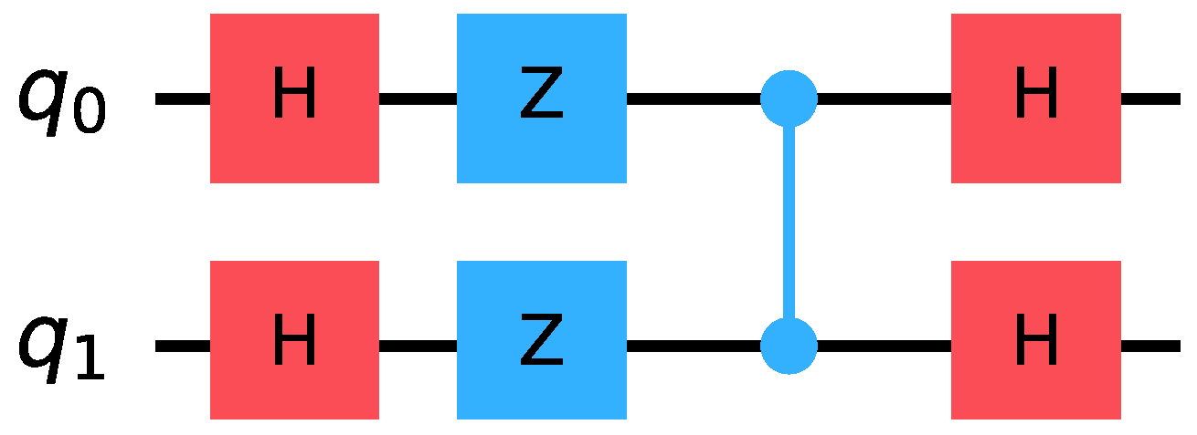In [38] it was shown that $C_2$, defined by the Equation (11), is the classifier for $Q_2$ and $F_{Q_2}$. The matrix representation of $C_2$ is given by Equation (12). It is quite easy to construct $C_2$ using standard quantum gates readily available in contemporary quantum computers, such as Hadamard, Z and controlled-Z gates, as demonstrated in Figure 3.

$$\begin{array}{c}\hfill C_2=(H\otimes H)CZ(Z\otimes Z)(H\otimes H)\hfill \end{array}$$

(11)

$$C_2=\left[\begin{array}{cccc}\hfill -{\displaystyle \frac{1}{2}}\hfill & \hfill \phantom{-}{\displaystyle \frac{1}{2}}\hfill & \hfill \phantom{-}{\displaystyle \frac{1}{2}}\hfill & \hfill \phantom{-}{\displaystyle \frac{1}{2}}\hfill \\ \hfill \phantom{-}{\displaystyle \frac{1}{2}}\hfill & \hfill -{\displaystyle \frac{1}{2}}\hfill & \hfill \phantom{-}{\displaystyle \frac{1}{2}}\hfill & \hfill \phantom{-}{\displaystyle \frac{1}{2}}\hfill \\ \hfill \phantom{-}{\displaystyle \frac{1}{2}}\hfill & \hfill \phantom{-}{\displaystyle \frac{1}{2}}\hfill & \hfill -{\displaystyle \frac{1}{2}}\hfill & \hfill \phantom{-}{\displaystyle \frac{1}{2}}\hfill \\ \hfill \phantom{-}{\displaystyle \frac{1}{2}}\hfill & \hfill \phantom{-}{\displaystyle \frac{1}{2}}\hfill & \hfill \phantom{-}{\displaystyle \frac{1}{2}}\hfill & \hfill -{\displaystyle \frac{1}{2}}\hfill \end{array}\right]$$

(12)

We introduce a mechanism for creating new pattern bases from existing ones, by utilizing the concept of product between pattern bit vectors and pattern bases.

Definition 9

(New Pattern Bases From Old).

If $\mathbf{p}$ = $p_{2^n-1}$…$p_1$$p_0$ and $\mathbf{q}$ = $q_{2^m-1}$…$q_1$$q_0$ are two pattern bit vectors of length $2^n$ and $2^m$, respectively, their product $\mathbf{p}\odot \mathbf{q}$ is pattern bit vector of length $2^{n+m}$ defined as

$$\begin{array}{c}\hfill \mathbf{p}\odot \mathbf{q}={\mathbf{s}}_{2^n-1}\dots {\mathbf{s}}_1{\mathbf{s}}_0,\mathit{where}{\mathbf{s}}_i=\left\{\begin{array}{cc}\hfill \mathbf{q}\hfill & \hfill \mathit{if}{p}_i=0\hfill \\ \hfill \overline{\mathbf{q}}\hfill & \hfill \mathit{if}{p}_i=1\hfill \end{array}\right.,0\le i\le 2^n-1.\hfill \end{array}$$

(13)

If $P_n$ = $({\mathbf{p}}_0,{\mathbf{p}}_1,$ …$,{\mathbf{p}}_{2^n-1})$ and $Q_m$ = $({\mathbf{q}}_0,$${\mathbf{q}}_1,$…, ${\mathbf{q}}_{2^m-1})$ are two pattern bases of rank n and m, respectively, their product $P_n$⊙$Q_m$ is a pattern basis containing $2^{n+m}$ pattern bit vectors, each of length $2^{n+m}$, which is constructed as

$$\begin{array}{cc}\hfill P_n\odot Q_m≔(& {\mathbf{p}}_0\odot {\mathbf{q}}_0,{\mathbf{p}}_0\odot {\mathbf{q}}_1,\dots ,{\mathbf{p}}_0\odot {\mathbf{q}}_{2^m-1},\hfill \\ \hfill \hfill & {\mathbf{p}}_1\odot {\mathbf{q}}_0,{\mathbf{p}}_1\odot {\mathbf{q}}_1,\dots ,{\mathbf{p}}_1\odot {\mathbf{q}}_{2^m-1},\hfill \\ \hfill \hfill & \dots ,\hfill \\ \hfill \hfill & {\mathbf{p}}_{2^n-1}\odot {\mathbf{q}}_0,{\mathbf{p}}_{2^n-1}\odot {\mathbf{q}}_1,\dots ,{\mathbf{p}}_{2^n-1}\odot {\mathbf{q}}_{2^m-1}).\hfill \end{array}$$

(14)

The use of same symbol ⊙ for the product operation between two pattern bit vectors, and between two pattern bases should cause no confusion because the context always makes clear the intended operation.

Example 4

(Example of Pattern Bases Product). This example is meant to illustrate how the product between two pattern bases is constructed. For simplicity, we compute the product of $Q_2$, defined by Equation (10), with itself.

$$Q_4≔Q_2\odot Q_2.$$

(15)

To explain the inner workings of Definition 9 works, we enumerate the elements of $Q_4$ in

Table 3. This table contains the pattern bit vectors of $Q_4$.

${\mathbf{Q}}_2$ Pattern Bit Vectors	${\mathbf{g}}_{\mathit{i}}\odot {\mathbf{g}}_0,0\le \mathit{i}\le 3$	${\mathbf{g}}_{\mathit{i}}\odot {\mathbf{g}}_1,0\le \mathit{i}\le 3$	${\mathbf{g}}_{\mathit{i}}\odot {\mathbf{g}}_2,0\le \mathit{i}\le 3$	${\mathbf{g}}_{\mathit{i}}\odot {\mathbf{g}}_3,0\le \mathit{i}\le 3$
${\mathbf{g}}_0=0001$	${\mathbf{r}}_0:0001000100011110$	${\mathbf{r}}_1:0010001000101101$	${\mathbf{r}}_2:0100010001001011$	${\mathbf{r}}_3:1000100010000111$
${\mathbf{g}}_1=0010$	${\mathbf{r}}_4:0001000111100001$	${\mathbf{r}}_5:0010001011010010$	${\mathbf{r}}_6:0100010010110100$	${\mathbf{r}}_7:1000100001111000$
${\mathbf{g}}_2=0100$	${\mathbf{r}}_8:0001111000010001$	${\mathbf{r}}_9:0010110100100010$	${\mathbf{r}}_{10}:0100101101000100$	${\mathbf{r}}_{11}:1000011110001000$
${\mathbf{g}}_3=1000$	${\mathbf{r}}_{12}:1110000100010001$	${\mathbf{r}}_{13}:1101001000100010$	${\mathbf{r}}_{14}:1011010001000100$	${\mathbf{r}}_{15}:0111100010001000$

, indicating their derivation from $Q_2$.

By inspecting the above Table 3, we may may immediately conclude that $Q_4$ satisfies the condition set in Definition 6, and is, therefore, a pattern basis of rank 4. Following Definition 7, we denote by $F_{Q_4}$ the class of Boolean functions that realizes the pattern basis $Q_4$.

In a symmetric manner, we present a method from constructing new function classes using the notion of external product.

Definition 10

(New Function Classes From Old).

If $f_{\mathbf{p}}:{\mathbb{B}}^n\to \mathbb{B}$ and $g_{\mathbf{q}}:{\mathbb{B}}^m\to \mathbb{B}$ are the Boolean functions realizing the pattern bit vectors $\mathbf{p}$ and $\mathbf{q}$, respectively, their extended product $f_{\mathbf{p}}★g_{\mathbf{q}}:{\mathbb{B}}^{n+m}\to \mathbb{B}$ is the Boolean function defined as

$$\begin{array}{c}\hfill f_{\mathbf{p}}★g_{\mathbf{q}}(j+i{2}^n)=\left\{\begin{array}{cc}\hfill g_{\mathbf{q}}\left(j\right)\hfill & \hfill \mathit{if}{f}_{\mathbf{p}}\left(i\right)=0\hfill \\ \hfill \overline{g_{\mathbf{q}}\left(j\right)}\hfill & \hfill \mathit{if}{f}_{\mathbf{p}}\left(i\right)=1\hfill \end{array}\right.,0\le i\le 2^n-1,0\le j\le 2^m-1.\hfill \end{array}$$

(16)

If $F_{P_n}$ = $(f_{{\mathbf{p}}_0},f_{{\mathbf{p}}_1},$ …$,f_{{\mathbf{p}}_{2^n-1}})$ and $F_{Q_m}$ = $(f_{{\mathbf{q}}_0},f_{{\mathbf{q}}_1},$ …$,f_{{\mathbf{q}}_{2^m-1}})$ are the classes of Boolean functions that realize the pattern bases $P_n$ and $Q_m$ of rank n and m, respectively, their extended product $F_{P_n}$★$F_{Q_m}$ is a class of $2^{n+m}$ Boolean functions, which is constructed as

$$\begin{array}{cc}\hfill F_{P_n}★F_{Q_m}≔(& f_{{\mathbf{p}}_0}★f_{{\mathbf{q}}_0},f_{{\mathbf{p}}_0}★f_{{\mathbf{q}}_1},\dots ,f_{{\mathbf{p}}_0}★f_{{\mathbf{q}}_{2^m-1}},\hfill \\ \hfill \hfill & f_{{\mathbf{p}}_1}★f_{{\mathbf{q}}_0},f_{{\mathbf{p}}_1}★f_{{\mathbf{q}}_1},\dots ,f_{{\mathbf{p}}_1}★f_{{\mathbf{q}}_{2^m-1}},\hfill \\ \hfill \hfill & \dots ,\hfill \\ \hfill \hfill & f_{{\mathbf{p}}_{2^n-1}}★f_{{\mathbf{q}}_0},f_{{\mathbf{p}}_{2^n-1}}★f_{{\mathbf{q}}_1},\dots ,f_{{\mathbf{p}}_{2^n-1}}★f_{{\mathbf{q}}_{2^m-1}}).\hfill \end{array}$$

(17)

In view of Definitions 9 and 10, it is straightforward to establish the following fact.

Proposition 1

(Extended Function Product Realizes Pattern Vector Product). If $f_{\mathbf{p}}:{\mathbb{B}}^n\to \mathbb{B}$ and $g_{\mathbf{q}}:{\mathbb{B}}^m\to \mathbb{B}$ are the Boolean functions realizing the pattern bit vectors $\mathbf{p}$ and $\mathbf{q}$, respectively, their extended product $f_{\mathbf{p}}★g_{\mathbf{q}}:{\mathbb{B}}^{n+m}\to \mathbb{B}$ is the Boolean function that realizes the pattern bit vector $\mathbf{p}\odot \mathbf{q}$.

Continuing this line of reasoning, we arrive at the next Theorem.

Theorem 1

(Extended Function Product Realizes Pattern Bases Product). If $F_{P_n}$ and $F_{Q_m}$ are the classes of Boolean functions that realize the pattern bases $P_n$ and $Q_m$ of rank n and m, respectively, their extended product $F_{P_n}$★$F_{Q_m}$ realized the pattern basis $P_n$⊙$Q_m$.

To ensure this investigation yields meaningful and reproducible results, it must be anchored in well-defined assumptions and a robust theoretical framework. To this end, we agree that the quantum classifiers we investigate in this work, are constructed as prescribed by the next Definition 11, using as elementary building blocks the Hadamard transform H and the classifier $C_2$, defined by Equation (11).

Definition 11

(Quantum Classifier). A quantum classifier $\mathbf{G}$ is a finite tensor product of the form

$$\begin{array}{c}\hfill \mathbf{G}=G_{m-1}\otimes \dots \otimes G_0,\hfill \end{array}$$

(18)

where each $G_j,0\le j\le m-1,$ is either the Hadamard transform H or the classifier $C_2$, defined by Equation (11).

Using induction on m, we may prove Theorem 2.

Theorem 2

(Classification of Products of Pattern Bases & Function Classes). Consider the quantum classifier $\mathbf{G}$ = $G_{m-1}$⊗…⊗$G_0$, where each $G_j,0\le j\le m-1,$ is the classifier for $P_j$ and $F_{P_j}$. Then $\mathbf{G}$ classifies the class of Boolean functions $F_{P_{m-1}}$★…★$F_{P_0}$ realizing the pattern basis $P_{m-1}$⊙…⊙$P_0$.

An immediate Corollary of the Theorem 2 is the following.

Corollary 1

(Correspondence among Bases, Function Classes & Classifiers). Let P be the product pattern bit basis

$$\begin{array}{c}\hfill P=P_{m-1}\odot \dots \odot P_0,\hfill \end{array}$$

(19)

where each $P_j,0\le j\le m-1,$ is either the basis $B_1$ or the basis $Q_2$, defined by Equations (9) and (10), respectively.

The class $F_P$ of Boolean functions that realizes P is the extended product

$$\begin{array}{c}\hfill F_P=F_{P_{m-1}}★\dots ★F_{P_0},\hfill \end{array}$$

(20)

where each $F_{P_j},0\le j\le m-1,$ is $F_{B_1}$ if $P_j=B_1$ or $F_{Q_2}$ if $P_j=Q_2$.

The quantum classifier $\mathbf{G}$ that classifies $F_P$ is the tensor product

$$\begin{array}{c}\hfill \mathbf{G}=G_{m-1}\otimes \dots \otimes G_0,\hfill \end{array}$$

(21)

where each $G_j,0\le j\le m-1,$ is H if $P_j=B_1$ or $C_2$ if $P_j=Q_2$.

Corollary 1 makes explicitly clear the one-to-one correspondence among pattern bases product, function classes extended product, and quantum classifiers tensor product.

Example 5

(Perfectly Classifiable Function in $F_{Q_4}$). Consider the pattern bit vector ${\mathbf{r}}_3=1000100010000111$∈$Q_4$, listed in Table 3 of Example 4. As shown there, ${\mathbf{r}}_3$ is the product ${\mathbf{g}}_0\odot {\mathbf{g}}_3$ of the pattern vectors ${\mathbf{g}}_0$ and ${\mathbf{g}}_3$, where ${\mathbf{g}}_0,{\mathbf{g}}_3\in Q_2$. By Theorem 1, the Boolean function $f_{{\mathbf{r}}_3}$ that realizes pattern bit vector ${\mathbf{r}}_3$ is extended product $f_{{\mathbf{r}}_3}$ = $f_{{\mathbf{g}}_0}★f_{g_3}$, where $f_{{\mathbf{g}}_0}$ and $f_{{\mathbf{g}}_3}$ are the functions realizing ${\mathbf{g}}_0$ and ${\mathbf{g}}_3$, respectively. From Example 3 we know that $C_2$, defined by Equation (11), is the classifier for the class of Boolean functions $F_{Q_2}$ that realizes the pattern basis $Q_2$. According to Theorem 2, $C_2\otimes C_2$ is the classifier for the class $F_{Q_2}$★$F_{Q_2}$ that realizes the pattern basis $Q_2$⊙$Q_2$. 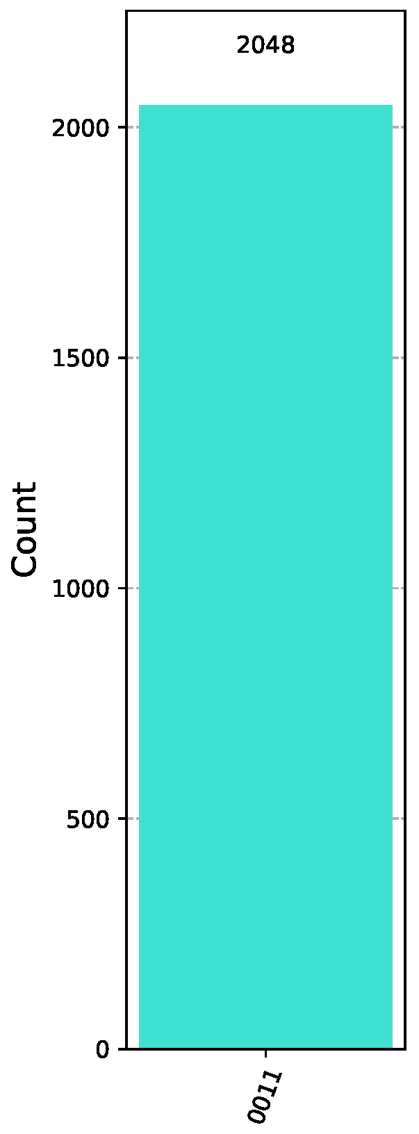In this scenario, the concrete implementation of the Pattern Basis Classification Scheme outlined in Definition 8 in Qiskit [47] is shown in Figure 4 below, where the oracle encodes $f_{{\mathbf{r}}_3}$.

Before measurement, the state of the system is just $|\mathbf{0011}\rangle$. Hence, measuring the quantum circuit depicted in Figure 4 will output the bit vector 0011 with probability 1. This is corroborated by the simulating this circuit in Qiskit for 2048 runs, as shown in Figure 5). The binary vector 0011 reveals the index of the function hidden in the oracle, namely $f_{{\mathbf{r}}_3}$. This provides a conclusive demonstration of the Pattern Basis Classification Scheme.

In general, if a quantum classifier $\mathbf{G}$ = $G_{m-1}$⊗…⊗$G_1$⊗$G_0$ classifies the class of Boolean functions $F_{P_n}$, then the quantum circuit visualized in Figure 6, where the oracle $U_f$ encodes a function $f\in F_{P_n}$, will conclusively, i.e., with probability 1, classify f. To enhance clarity, we explain the notation used in Figure 6.

• $IR$ is the quantum input register that contains n qubits and starts its operation at state $|\mathbf{0}\rangle$.
• $OR$ is the single-qubit output register initialized to |−〉.
• H is the Hadamard transform.
• $U_f$ is the unitary transform corresponding to the oracle for the unknown function f. The latter is promised to be an element of $F_{P_n}$.
• $G_j,0\le j\le m-1,$ are the fundamental building blocks of $\mathbf{G}$ = $G_{m-1}$⊗…⊗$G_1$⊗$G_0$ classifying the class of Boolean functions $F_{P_n}$.

We now emphasize an important point regarding the behavior of classification algorithms on general inputs. No classification algorithm is expected to produce correct results—and is unlikely to do so—for Boolean functions that fall outside the class of perfectly classifiable functions. Thus, regarding the quantum circuit of Figure 6, if the oracle realizes a function outside $F_{P_n}$, the final measurement, may not reveal the unknown function. In the rest of this paper, we investigate whether, and under what assumptions, it is possible to obtain some useful information when the input function is close to the class $F_{P_n}$.

4. What About Nonclassifiable Boolean Functions?

In view of the last remark of the previous Section, we lay down the objectives of this study. Let us assume that we have fixed the class of Boolean functions $F_{P_n}$ that realizes the pattern basis $P_n$, and that $\mathbf{G}$ is the classifier for $F_{P_n}$ and $P_n$. In the rest of this paper we investigate the following questions.

• When the input function h is nonclassifiable by $\mathbf{G}$, i.e., $h\notin F_{P_n}$, is it possible, and under what conditions, to obtain some useful information about h?
• By useful information we mean to learn as much as possible about the behavior of h. Within the current framework, this translates to knowing (one of) the $f\in F_{P_n}$ “nearest” to h.
• Thus, to quantify the “nearness” between two Boolean functions, a notion of distance is required. In this work, we adopt one of the most general distance metric, the Hamming distance.
• Finally, we aim to answer the question of how useful is the Hamming distance, as defined in Definition 12, for classification purposes.

Undoubtedly, any attempt to arrive at quantitative conclusions, presupposes a metric to capture the notion of “closeness” or distance between two Boolean functions. As mentioned above, in this study we employ one of the most conventional and most general distance metrics, namely the Hamming distance (see [48,49]), and analyze its benefits and drawbacks. In [46] a totally different concept of distance, based on left and right clusters, was used. The classification game investigated there, with the distance restriction forcing the unknown function to be either in the left or right cluster of a perfectly classifiable function, enabled Alice to surely win. The Nearest Basis Ket Game we study in this work is totally different because it deals with the utmost general situation where Bob can pick any Boolean function with no restrictions whatsoever.

Definition 12

(Hamming Distance of Boolean Functions). Let f and h be two Boolean functions from ${\mathbb{B}}^n\to \mathbb{B}$, and let ${\mathbf{p}}_f$ and ${\mathbf{p}}_h$ be their corresponding pattern bit vectors. We define the Hamming distance between f and h, denoted $d_H(f,h)$, as follows:

$$\begin{array}{c}\hfill d_H(f,h)≔d_H({\mathbf{p}}_f,{\mathbf{p}}_h).\hfill \end{array}$$

(22)

Definition 13

(Neighborhoods of Boolean Functions). Let f be a Boolean function from ${\mathbb{B}}^n\to \mathbb{B}$. The r-neighborhood of f, denoted by $N_r\left(f\right)$, $r\ge 0$, is the collection of all Boolean functions h from ${\mathbb{B}}^n\to \mathbb{B}$ such that $d_H(f,h)\le r$.

Definition 14

(Hamming Distance from Function Class). Given the class of Boolean functions $F_{P_n}$ that realizes the pattern basis $P_n$, and an arbitrary Boolean function $h:{\mathbb{B}}^n\to \mathbb{B}$, $n\ge 1$, the Hamming distance of h from $F_{P_n}$, denoted by $d_H(F_{P_n},h)$, is defined as

$$\begin{array}{c}\hfill d_H(F_{P_n},h)=min\{d:d=d_H(f,h),f\in F_{P_n}\}.\hfill \end{array}$$

(23)

Definition 15

(Nearest Neighbors in Function Class). Given the class of Boolean functions $F_{P_n}$ that realizes the pattern basis $P_n$, and an arbitrary Boolean function $h:{\mathbb{B}}^n\to \mathbb{B}$, $n\ge 1$, the nearest neighbors of h in $F_{P_n}$, denoted by $NN(F_{P_n},h)$, are the Boolean functions $f\in F_{P_n}$ such that $d_H(f,h)=d_H(F_{P_n},h)$.

Definition 16

(Nearest Basis Kets). Let $\mathbf{G}$ be a quantum classifier for the class of Boolean functions $F_{P_n}$ realizing the pattern basis $P_n$. Given an arbitrary Boolean function $h:{\mathbb{B}}^n\to \mathbb{B}$, not in $F_{P_n}$, let $NN(F_{P_n},h)=\{f_{{\mathbf{p}}_{i_1}},f_{{\mathbf{p}}_{i_2}},\dots ,f_{{\mathbf{p}}_{i_r}}\}$ be the collection of nearest neighbors of h in $F_{P_n}$.

The nearest basis kets of h in $F_{P_n}$, denoted by $NK(F_{P_n},h)$, are the basis kets $\left\{\right|{\mathbf{i}}_1\rangle ,|{\mathbf{i}}_2\rangle ,\dots ,|{\mathbf{i}}_r\rangle \}$, where $|{\mathbf{i}}_1\rangle ,|{\mathbf{i}}_2\rangle ,\dots ,|{\mathbf{i}}_r\rangle$ are the classification measurements for $f_{{\mathbf{p}}_{i_1}},f_{{\mathbf{p}}_{i_2}},\dots ,f_{{\mathbf{p}}_{i_r}}$ according to the Pattern Basis Classification Scheme outlined in Definition 8.

The classification threshold ϑ of h is the probability that $CM\left(h\right)$ belongs to $NK(F_{P_n},h)$.

Example 6

(The Hamming Distance of g from $F_{Q_4}$). Let us consider the pattern bit vector ${\mathbf{r}}_0=0001000100011110$∈$Q_4$, listed in Table 3 of Example 4, and the pattern vector ${\mathbf{p}}_g=0000000100011110$ encountered in Example 1. The values of the corresponding Boolean functions $f_{{\mathbf{r}}_0}$ and g are contained in

Table 4. Comparison between the truth values of the functions g and $f_0$.

	0000	0001	0010	0011	0100	0101	0110	0111	1000	1001	1010	1011	1100	1101	1110	1111
g	0	1	1	1	1	0	0	0	1	0	0	0	0	0	0	0
$f_{{\mathbf{r}}_0}$	0	1	1	1	1	0	0	0	1	0	0	0	1	0	0	0

. A comparison between their corresponding values shows that they only differ in the values the assume at input $\mathbf{x}=1100$, where $f_{{\mathbf{r}}_0}\left(\mathbf{x}\right)=1$ whereas $g\left(\mathbf{x}\right)=0$. According to Definition 12, $d_H(f_{{\mathbf{r}}_0},g)=1$. By systematically going over all other functions of the class $F_{Q_4}$, we immediately verify that their distance from g is $>1$. Therefore, $NN(F_{Q_4},g)$ = $\left\{f_{{\mathbf{r}}_0}\right\}$. Lastly, taking into account the Pattern Basis Classification Scheme outlined in Definition 8 and Definition 16, we conclude that the nearest basis ket of g in $F_{Q_4}$ is |0000〉, or, in other words, $NK(F_{Q_4},h)$ = $\left\{\right|0000\rangle \}$.

To make this investigation more intuitive and engaging, we conceptualize the classification process as a strategic interaction, formalized as a game between two players, Alice and Bob, whom we cast as our talented protagonists. This game, termed the Nearest Basis Ket Game, encapsulates the challenge of identifying one of the “closest” functions in $F_{P_n}$ to an unknown function h. The rules of the game are as follows:

(R1) Alice and Bob fix a classifier $\mathbf{G}$ and the corresponding class of Boolean functions $F_P$ that realizes the pattern basis P. (R2) Bob picks an arbitrary Boolean function h that doesn’t belong to $F_P$ and reveals to Alice only the minimum Hamming distance of h from $F_P$. (R3) Bob implements the abstract classification circuit of Figure 2 using the oracle for h, and announces the classification measurement $CM\left(h\right)$ to Alice. (R4) The challenge posed to Alice is to decide whether $CM\left(h\right)$ belongs to $NK(F_P,h)$. (R5) Alice wins the game if she gives the correct answer, either yes or no, to the above question, otherwise Bob is declared the winner.

As we show in the rest of this paper, when the Hamming distance lies within certain intervals, the question whether $CM\left(h\right)\in NK(F_{P_n},h)$ can be answered affirmatively or negatively with high probability.

5. What Do Experiments Show?

5.1. Experimental Methodology

To evaluate the usefulness of the Hamming distance as a meaningful metric to measure “closeness” between Boolean functions, we have conducted a series of experiments using Qiskit [47]. This Section is devoted to the presentation and analysis of these experiments. Our experimental methodology was meticulously designed to uphold the core principles of

• reproducibility, and
• interpretability,

ensuring that all procedures, parameters, and outcomes could be reliably replicated by independent researchers while providing clear, transparent explanations for the observed phenomena. To achieve this, we documented every step in detail, alongside comprehensive logging of intermediate results and computational traces. The experiments and their subsequent analysis and interpretation were executed within a period of several months, during which the quantum computing landscape and associated software tools continued to evolve. Throughout the experimental runs, different editions of the Qiskit platform [47] were employed to accommodate updates and improvements in the framework: the initial Qiskit version deployed at the commencement of the experimental phase was 1.4.2, while the experiments were ultimately concluded using the more advanced version 2.1.2. It is worth noting that at the time of writing this manuscript, the most recent stable Qiskit version available is 2.2.3, and the latest release candidate is Qiskit 2.3.0rc1, reflecting the continued rapid development in this field.

We clarify the experimental setup used throughput this series of experiments. For each experiment we fix a quantum classifier $\mathbf{G}=G_{m-1}\otimes \dots \otimes G_0$, where each factor of the tensor product is one of the elementary classifiers H or $C_2$. For the chosen $\mathbf{G}$, the class of perfectly classifiable Boolean functions $F_P$ and the pattern basis P realized by this class are unambiguously specified, as prescribed by Theorem 2 and Corollary 1. The Pattern Basis Classification Scheme is achieved via the appropriate implementation of the abstract quantum circuit depicted in Figure 6. Our experiments shed light on the following question.

Experimental Investigation

Assuming that the oracle in Figure 6 encodes an unknown random function h, what is the classification threshold of h, that is what is probability that the classification measurement $CM\left(h\right)$ belongs to $NK(F_P,h)$, as a function of the Hamming distance $d_H(F_P,h)$ of h from $F_P$?

Given the inherent computational constraints—such as finite memory capacity and processing time—we adopted a pragmatic and scalable approach that balanced thoroughness with feasibility. For smaller-scale analyses, we performed an exhaustive enumeration of all possible Boolean functions associated with pattern bit vectors of length up to 16 bits. This comprehensive sweep covered the full combinatorial space of all $2^{16}$ = 65,536 functions from ${\mathbb{B}}^4\to \mathbb{B}$, which is quite manageable on modern hardware, allowing us to derive definitive insights without sampling biases.

For larger pattern bit vectors (lengths of 32 bits and beyond), exhaustive enumeration becomes prohibitively expensive due to the exponential growth in complexity. For instance, we have $2^{32}$ = 4,294,967,296 Boolean functions ${\mathbb{B}}^5\to \mathbb{B}$. Therefore, we shifted to a statistically robust sampling strategy. Specifically, we randomly generated a diverse set of pattern bit vectors using uniform distribution, ensuring broad coverage of the search space. For each generated vector, we systematically constructed the corresponding Boolean function and classified it under our experimental framework. This random sampling not only mitigated the risks of exhaustive computation but also enabled us to identify representative trends and generalize findings to the broader landscape of Hamming distance usability.

5.2. The Case of Exhaustively Enumerating All Boolean Functions

This case documents the behavior of all pattern bit vectors of length 8 and 16, which were fully enumerated and tested. In particular, using the elementary pattern bases $B_1$ and $Q_2$, defined by Equations (9) and (10) respectively, we constructed all possible products of pattern bases that consist of bit vectors of length 8 and 16. As explained in detail in Example 3, the function classes $F_{B_1}$ and $F_{Q_2}$ realize $B_1$ and $Q_2$. Thus, by invoking Corollary 1 that makes explicit the one-to-one exact correspondence among the products of bases, function classes, and quantum classifiers, we obtain the following results.

We begin the presentation of the experimental results with the pattern bases that contain bit vectors of length 8. The experimental results for the three classes of Boolean functions contained in

Table 5. This table contains the pattern bases that contain pattern bit vectors of length 8.

Pattern Bit Vector Length	Pattern Basis	Class of Classifiable Boolean Functions	Quantum Classifier
8	$B_1\odot B_1\odot B_1$	$F_{B_1}★F_{B_1}★F_{B_1}$	$H\otimes H\otimes H$
8	$B_1\odot Q_2$	$F_{B_1}★F_{Q_2}$	$H\otimes C_2$
8	$Q_2\odot B_1$	$F_{Q_2}★F_{B_1}$	$C_2\otimes H$

are virtually identical and this conclusion is summarized in the following text box. Hence, in Figure 7 we have chosen to display only the results for the class $F_{B_1}★F_{Q_2}$.

Conclusion for the pattern bit vectors of length 8

The probability distribution of the classification threshold is virtually identical for the function classes $F_{B_1}★F_{B_1}★F_{B_1}$, $F_{B_1}★F_{Q_2}$, and $F_{Q_2}★F_{B_1}$.

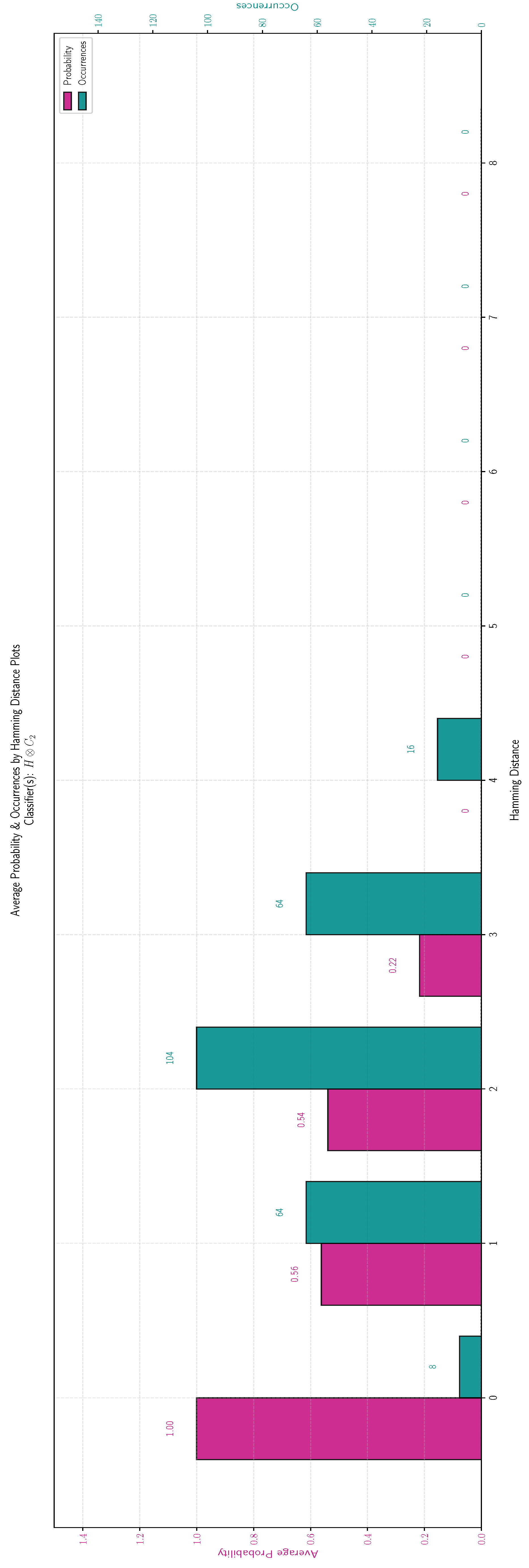
This particular scenario includes the class of Boolean functions $F_{B_1}★F_{Q_2}$ that realizes the pattern basis $B_1\odot Q_2$. In the histogram of Figure 7 the red bar depicts the classification threshold of a random h as a function of the Hamming distance $d_H(F_{B_1}★F_{Q_2},h)$ of h from $F_{B_1}★F_{Q_2}$. The green bar shows the number of Boolean Functions for which the Hamming distance from $F_{B_1}★F_{Q_2}$ takes a specific value. As we have emphasized, the results are identical for all three function classes and are summarized in

Table 6. The probability distribution of the classification threshold as a function of the Hamming distance for the classes $F_{B_1}★F_{B_1}★F_{B_1}$, $F_{B_1}★F_{Q_2}$, and $F_{Q_2}★F_{B_1}$ in tabular form.

	Classification Threshold $\mathit{\vartheta }$
Hamming Distance	${\mathit{F}}_{{\mathit{B}}_{\mathbf{1}}}★{\mathit{F}}_{{\mathit{B}}_{\mathbf{1}}}★{\mathit{F}}_{{\mathit{B}}_{\mathbf{1}}}$, ${\mathit{F}}_{{\mathit{B}}_{\mathbf{1}}}★{\mathit{F}}_{{\mathit{Q}}_{\mathbf{2}}}$, and  ${\mathit{F}}_{{\mathit{Q}}_{\mathbf{2}}}★{\mathit{F}}_{{\mathit{B}}_{\mathbf{1}}}$
1	$0.56$
2	$0.54$
3	$0.22$
$4,5,6,7,8$	0

.

We continue with the experimental results for the pattern bases with bit vectors of length 16 contained in

Table 7. This table contains the pattern bases that contain pattern bit vectors of length 16.

Pattern Bit Vector Length	Pattern Basis	Class of Classifiable Boolean Functions	Quantum Classifier
16	$B_1\odot B_1\odot B_1\odot B_1$	$F_{B_1}★F_{B_1}★F_{B_1}★F_{B_1}$	$H\otimes H\otimes H\otimes H$
16	$B_1\odot B_1\odot Q_2$	$F_{B_1}★F_{B_1}★F_{Q_2}$	$H\otimes H\otimes C_2$
16	$B_1\odot Q_2\odot B_1$	$F_{B_1}★F_{Q_2}★F_{B_1}$	$H\otimes C_2\otimes H$
16	$Q_2\odot B_1\odot B_1$	$F_{Q_2}★F_{B_1}★F_{B_1}$	$C_2\otimes H\otimes H$
16	$Q_2\odot Q_2$	$F_{Q_2}★F_{Q_2}$	$C_2\otimes C_2$

. Although, for bit vectors of length 8 the results are virtually identical, this time we observe a very interesting variation. This confirms our intuition that the characteristic traits of the specific pattern vectors comprising the basis affect in a most interesting way the probability distribution. The conclusion for this scenario is summarized in the next text box.

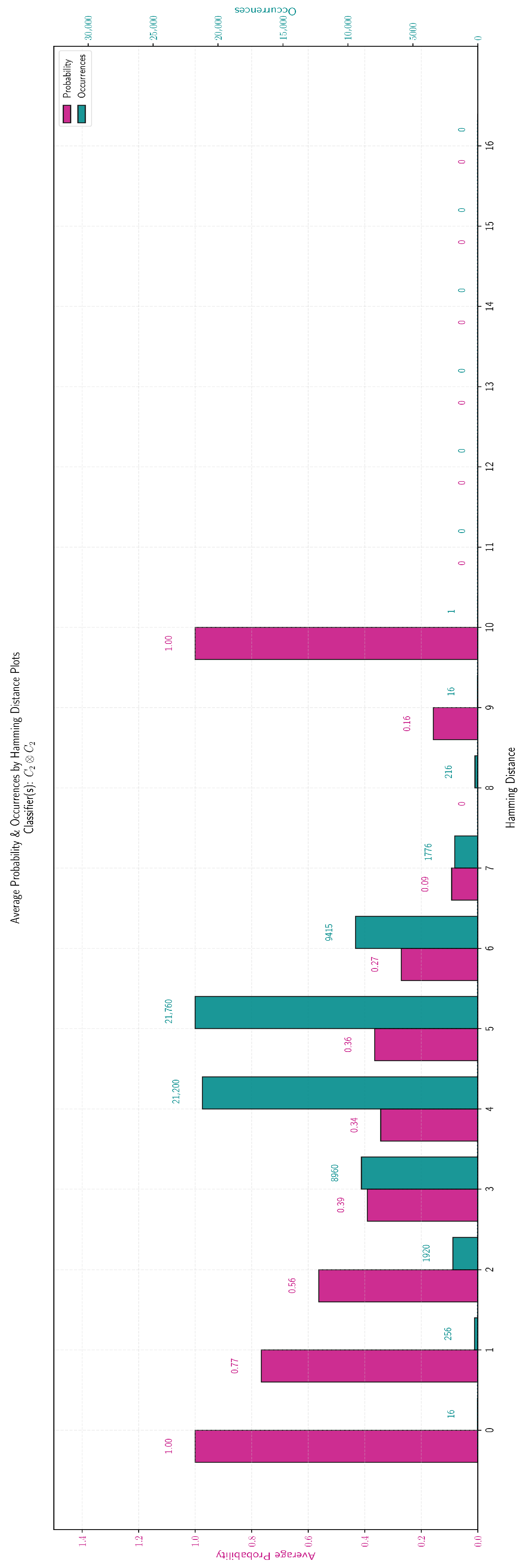
Figure 8 displays the results for the class $F_{B_1}★F_{Q_2}★F_{B_1}$, as representative of the first category above, while Figure 9 displays the results for the class $F_{Q_2}★F_{Q_2}$. According to our convention, in all Figures the red bars display probability values, whereas the green bars show the number of Boolean functions per distance. The results are contained in

Table 8. The probability distribution of the classification threshold as a function of the Hamming distance for the classes $F_{B_1}★F_{B_1}★F_{B_1}★F_{B_1}$, $F_{B_1}★F_{B_1}★F_{Q_2}$, $F_{B_1}★F_{Q_2}★F_{B_1}$, $F_{Q_2}★F_{B_1}★F_{B_1}$, and $F_{Q_2}★F_{Q_2}$ in tabular form.

	Classification Threshold $\mathit{\vartheta }$
Hamming Distance	${\mathit{F}}_{{\mathit{B}}_{\mathbf{1}}}★{\mathit{F}}_{{\mathit{B}}_{\mathbf{1}}}★{\mathit{F}}_{{\mathit{B}}_{\mathbf{1}}}★{\mathit{F}}_{{\mathit{B}}_{\mathbf{1}}}$, ${\mathit{F}}_{{\mathit{B}}_{\mathbf{1}}}★{\mathit{F}}_{{\mathit{B}}_{\mathbf{1}}}★{\mathit{F}}_{{\mathit{Q}}_{\mathbf{2}}}$, ${\mathit{F}}_{{\mathit{B}}_{\mathbf{1}}}★{\mathit{F}}_{{\mathit{Q}}_{\mathbf{2}}}★{\mathit{F}}_{{\mathit{B}}_{\mathbf{1}}}$, and  ${\mathit{F}}_{{\mathit{Q}}_{\mathbf{2}}}★{\mathit{F}}_{{\mathit{B}}_{\mathbf{1}}}★{\mathit{F}}_{{\mathit{B}}_{\mathbf{1}}}$	${\mathit{F}}_{{\mathit{Q}}_{\mathbf{2}}}★{\mathit{F}}_{{\mathit{Q}}_{\mathbf{2}}}$
1	$0.76$	$0.77$
2	$0.56$	$0.56$
3	$0.39$	$0.39$
4	$0.34$	$0.34$
5	$0.36$	$0.36$
6	$0.27$	$0.27$
7	$0.10$	$0.09$
8	0	0
9	0	$0.16$
10	0	1
$11,12,\dots ,16$	0	0

. The class $F_{Q_2}★F_{Q_2}$ exhibits a distinctly different classification threshold compared to the other four classes $F_{B_1}★F_{B_1}★F_{B_1}$, $F_{B_1}★F_{Q_2}$, and $F_{Q_2}★F_{B_1}$ because of the nonzero values at distances 9 and 10. It is worth noting that for distance 10, in particular, the classification threshold becomes 1. The reason for this behavior will be explained in Section 5.4.

Conclusion for the pattern bit vectors of length $\mathbf{16}$

The probability distribution of the classification threshold $\vartheta$ is virtually identical for the function classes $F_{B_1}★F_{B_1}★F_{B_1}★F_{B_1}$, $F_{B_1}★F_{B_1}★F_{Q_2}$, $F_{B_1}★F_{Q_2}★F_{B_1}$, and $F_{Q_2}★F_{B_1}★F_{B_1}$ and closely mirrors the shape encountered in the case of bit vectors of length 8. For the class $F_{Q_2}★F_{Q_2}$ the probability distribution of the classification threshold $\vartheta$ exhibits a different probability distribution with nonzero probability values for Hamming distances 9 and 10.

5.3. The Case of Sampling Boolean Functions

This case investigates the behavior of sampled pattern bit vectors of length 32 and 64. For such bit vectors, exhaustive enumeration becomes inefficient and impractical due to the exponential growth in complexity. Thus, we employed sampling by randomly generating a set of pattern bit vectors. For each generated vector, we constructed the corresponding Boolean function and oracle in order to classify via the Pattern Basis Classification Scheme outlined in Definition 8. This random sampling approach allowed us to generalize our findings regarding Hamming distance usability. As before, the elementary pattern bases $B_1$ and $Q_2$, defined by Equations (9) and (10) respectively, are the fundamental building blocks for the construction of all possible products of pattern bases that comprise bit vectors of length 32 and 64. Corollary 1 elucidates the one-to-one exact correspondence among the products of bases, function classes, and quantum classifiers, leading to the following results shown in

Table 9. This table contains the pattern bases that contain pattern bit vectors of length 32.

Pattern Bit Vector Length	Pattern Basis	Class of Classifiable Boolean Functions	Quantum Classifier
32	$B_1\odot B_1\odot B_1\odot B_1\odot B_1$	$F_{B_1}★F_{B_1}★F_{B_1}★F_{B_1}★F_{B_1}$	$H\otimes H\otimes H\otimes H\otimes H$
32	$B_1\odot B_1\odot B_1\odot Q_2$	$F_{B_1}★F_{B_1}★F_{B_1}★F_{Q_2}$	$H\otimes H\otimes H\otimes C_2$
32	$B_1\odot B_1\odot Q_2\odot B_1$	$F_{B_1}★F_{B_1}★F_{Q_2}★F_{B_1}$	$H\otimes H\otimes C_2\otimes H$
32	$B_1\odot Q_2\odot B_1\odot B_1$	$F_{B_1}★F_{Q_2}★F_{B_1}★F_{B_1}$	$H\otimes C_2\otimes H\otimes H$
32	$Q_2\odot B_1\odot B_1\odot B_1$	$F_{Q_2}★F_{B_1}★F_{B_1}★F_{B_1}$	$C_2\otimes H\otimes H\otimes H$
32	$B_1\odot Q_2\odot Q_2$	$F_{B_1}★F_{Q_2}★F_{Q_2}$	$H\otimes C_2\otimes C_2$
32	$Q_2\odot B_1\odot Q_2$	$F_{Q_2}★F_{B_1}★F_{Q_2}$	$C_2\otimes H\otimes C_2$
32	$Q_2\odot Q_2\odot B_1$	$F_{Q_2}★F_{Q_2}★F_{B_1}$	$C_2\otimes C_2\otimes H$

.

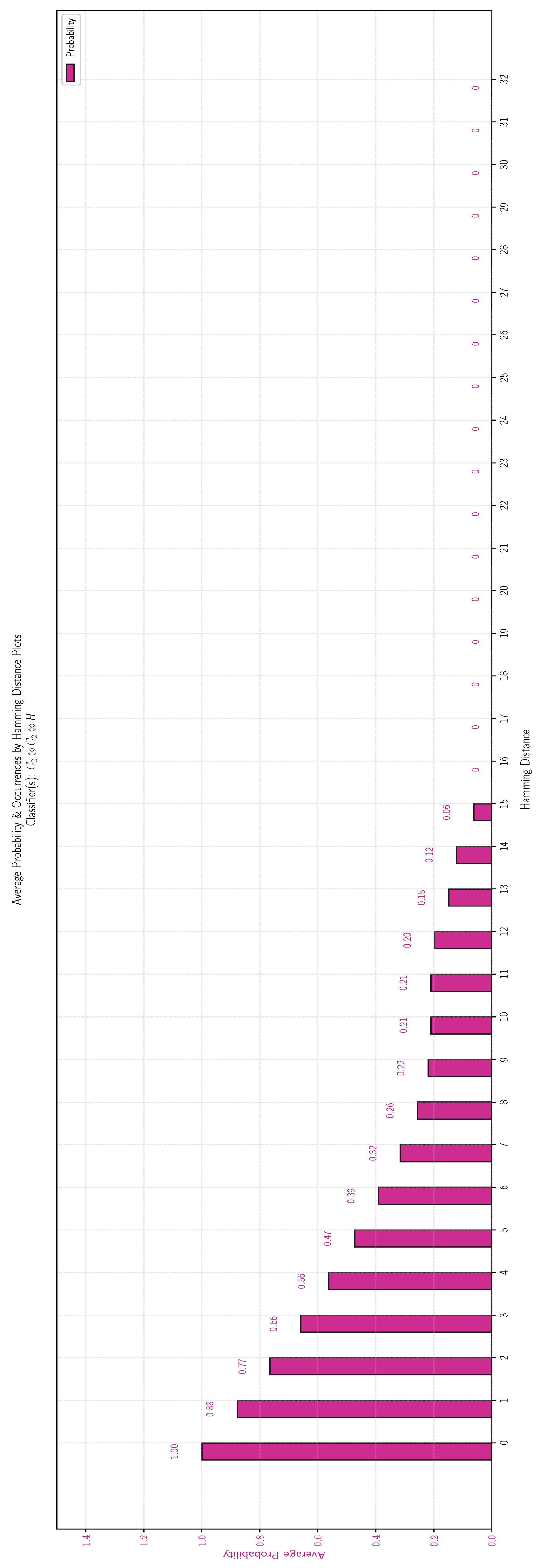
The experimental results corroborate that all the above function classes have a virtually identical probability distribution of the classification threshold. Hence, this series of experiments confirms the pattern already observed, i.e., that the classification threshold is a decreasing function of the Hamming distance.

Conclusion for the pattern bit vectors of length $\mathbf{32}$

The probability distribution for the classification threshold is the same for all the function classes $F_{B_1}★F_{B_1}★F_{B_1}★F_{B_1}★F_{B_1}$, $F_{B_1}★F_{B_1}★F_{B_1}★F_{Q_2}$, $F_{B_1}★F_{B_1}★F_{Q_2}★F_{B_1}$, $F_{B_1}★F_{Q_2}★F_{B_1}★F_{B_1}$, $F_{Q_2}★F_{B_1}★F_{B_1}★F_{B_1}$, $F_{B_1}★F_{Q_2}★F_{Q_2}$, $F_{Q_2}★F_{B_1}★F_{Q_2}$, and $F_{Q_2}★F_{Q_2}★F_{B_1}$.

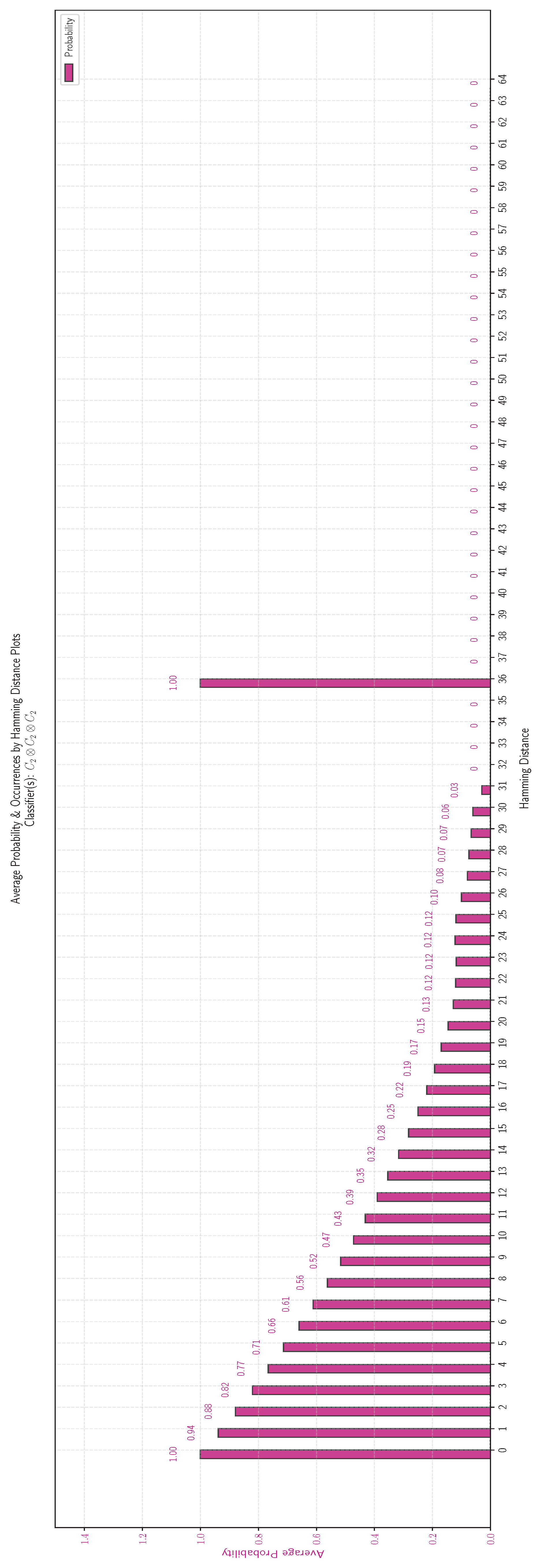
For this reason we illustrate only the results for the class $F_{Q_2}★F_{Q_2}★F_{B_1}$ in Figure 10. For enhanced readability, these results are repeated in tabular form in

Table 10. The probability distribution of the classification threshold as a function of the Hamming distance for the classes $F_{B_1}★F_{B_1}★F_{B_1}★F_{B_1}★F_{B_1}$, $F_{B_1}★F_{B_1}★F_{B_1}★F_{Q_2}$, $F_{B_1}★F_{B_1}★F_{Q_2}★F_{B_1}$, $F_{B_1}★F_{Q_2}★F_{B_1}★F_{B_1}$, $F_{Q_2}★F_{B_1}★F_{B_1}★F_{B_1}$, $F_{B_1}★F_{Q_2}★F_{Q_2}$, $F_{Q_2}★F_{B_1}★F_{Q_2}$, and $F_{Q_2}★F_{Q_2}★F_{B_1}$ in tabular form.

	Classification Threshold $\mathit{\vartheta }$
Hamming Distance	${\mathit{F}}_{{\mathit{B}}_{\mathbf{1}}}★{\mathit{F}}_{{\mathit{B}}_{\mathbf{1}}}★{\mathit{F}}_{{\mathit{B}}_{\mathbf{1}}}★{\mathit{F}}_{{\mathit{B}}_{\mathbf{1}}}★{\mathit{F}}_{{\mathit{B}}_{\mathbf{1}}}$, ${\mathit{F}}_{{\mathit{B}}_{\mathbf{1}}}★{\mathit{F}}_{{\mathit{B}}_{\mathbf{1}}}★{\mathit{F}}_{{\mathit{B}}_{\mathbf{1}}}★{\mathit{F}}_{{\mathit{Q}}_{\mathbf{2}}}$, ${\mathit{F}}_{{\mathit{B}}_{\mathbf{1}}}★{\mathit{F}}_{{\mathit{B}}_{\mathbf{1}}}★{\mathit{F}}_{{\mathit{Q}}_{\mathbf{2}}}★{\mathit{F}}_{{\mathit{B}}_{\mathbf{1}}}$, ${\mathit{F}}_{{\mathit{B}}_{\mathbf{1}}}★{\mathit{F}}_{{\mathit{Q}}_{\mathbf{2}}}★{\mathit{F}}_{{\mathit{B}}_{\mathbf{1}}}★{\mathit{F}}_{{\mathit{B}}_{\mathbf{1}}}$, ${\mathit{F}}_{{\mathit{Q}}_{\mathbf{2}}}★{\mathit{F}}_{{\mathit{B}}_{\mathbf{1}}}★{\mathit{F}}_{{\mathit{B}}_{\mathbf{1}}}★{\mathit{F}}_{{\mathit{B}}_{\mathbf{1}}}$, ${\mathit{F}}_{{\mathit{B}}_{\mathbf{1}}}★{\mathit{F}}_{{\mathit{Q}}_{\mathbf{2}}}★{\mathit{F}}_{{\mathit{Q}}_{\mathbf{2}}}$, ${\mathit{F}}_{{\mathit{Q}}_{\mathbf{2}}}★{\mathit{F}}_{{\mathit{B}}_{\mathbf{1}}}★{\mathit{F}}_{{\mathit{Q}}_{\mathbf{2}}}$, and ${\mathit{F}}_{{\mathit{Q}}_{\mathbf{2}}}★{\mathit{F}}_{{\mathit{Q}}_{\mathbf{2}}}★{\mathit{F}}_{{\mathit{B}}_{\mathbf{1}}}$
$1,\dots ,4$	$0.50<\vartheta <1$
$5,\dots ,15$	$0<\vartheta <0.50$
$16,\dots ,32$	0

.

The fact that the classification of random functions with respect to their nearest neighbors in all the above function classes follows the same pattern, is a strong indication of the robustness of our results. A small deviation from this dominating behavior is observed when the function class is $F_{Q_2}★F_{Q_2}$. To test whether this is a statistical artifact or something inherent in classes that are obtained as the external product of the same factor $F_{Q_2}$, we have experimented with the class $F_{Q_2}★F_{Q_2}★F_{Q_2}$, as shown in

Table 11. This table shows the class $F_{Q_2}★F_{Q_2}★F_{Q_2}$ that realizes the pattern basis $Q_2\odot Q_2\odot Q_2$ consisting of pattern bit vectors of length 64.

Pattern Bit Vector Length	Pattern Basis	Class of Classifiable Boolean Functions	Quantum Classifier
64	$Q_2\odot Q_2\odot Q_2$	$F_{Q_2}★F_{Q_2}★F_{Q_2}$	$C_2\otimes C_2\otimes C_2$

. The results for the class $F_{Q_2}★F_{Q_2}★F_{Q_2}$ are presented in Figure 11. The conclusion we have arrived at is given below. For clarity, the results are repeated in tabular form in

Table 12. The probability distribution of the classification threshold as a function of the Hamming distance for the class $F_{Q_2}★F_{Q_2}★F_{Q_2}$ in tabular format.

	Classification Threshold $\mathit{\vartheta }$
Hamming Distance	${\mathit{F}}_{{\mathit{Q}}_{\mathbf{2}}}★{\mathit{F}}_{{\mathit{Q}}_{\mathbf{2}}}★{\mathit{F}}_{{\mathit{Q}}_{\mathbf{2}}}$
$1,\dots ,9$	$0.50<\vartheta <1$
$9,\dots ,31$	$0<\vartheta <0.50$
$32,\dots ,35$	0
36	1
$37,\dots ,64$	0

.

Conclusion for the pattern bit vectors of length $\mathbf{64}$

For the most part, the probability distribution of the classification threshold of a random function h with respect to the class $F_{Q_2}★F_{Q_2}★F_{Q_2}$ is similar to that of other class, i.e., a decreasing function of the Hamming distance. However, there is a noteworthy difference at Hamming distance 36, where, instead of being 0, it spikes to 1.

In the coming Section, we interpret the results and provide an explanation regarding the probability spike observed when the product function class is constructed entirely by factors of the class $F_{Q_2}$.

5.4. Interpretation of the Experimental Results

By synthesizing the comprehensive experimental outcomes, a definitive pattern emerges: within an arbitrary function class, the classification threshold manifests as a monotonically decreasing function with respect to the Hamming distance. This trend, while robust across diverse scenarios, is complicated by predictable anomalies in certain specialized configurations, allowing us to articulate a foundational “rule” tempered by precisely delineated exceptions. To formalize this insight, we introduce the parameter n, representing the arity of the Boolean functions mapping ${\mathbb{B}}^n\to \mathbb{B}$ within a given class $F_P$, alongside the vector length $2^n$ of the pattern bit vectors that constitute the associated pattern basis P. This framework enables the specification of subintervals that systematically partition the full spectrum from 0 to $2^n$ into three regions, as illustrated in

Table 13. This table gives the probability distribution of the classification threshold as a function of the Hamming distance for a general class $F_P$, and for a special class $F_{Q_2}^{\otimes m}$. The results are parameterized by n, the arity of the Boolean functions in the class.

	Classification Threshold $\mathit{\vartheta }$
Hamming Distance	${\mathit{F}}_{\mathit{P}}$	${\mathit{F}}_{{\mathit{Q}}_{\mathbf{2}}}^{\otimes \mathit{m}}$
$1,\dots ,{\displaystyle \frac{2^n}{8}}$	$0.50<\vartheta <1$	$0.50<\vartheta <1$
${\displaystyle \frac{2^n}{8}}+1,\dots ,{\displaystyle \frac{2^n}{2}}-1$	$0<\vartheta <0.50$	$0<\vartheta <0.50$
${\displaystyle \frac{2^n}{2}},\dots ,\varrho -1$	0	0
$\varrho$	0	1
$\varrho +1,\dots ,2^n$	0	0

. Notably, when the function class is an extended product of the form $F_{Q_2}^{\otimes m}$, for some $m\ge 1$, a pronounced irregularity arises in the third region, manifesting as a sharp peak where the probability surges to precisely 1—a departure that underscores the nuanced interplay between structural properties and probabilistic outcomes.

This distinctive anomaly can be traced to an intrinsic hallmark of the functions populating $F_{Q_2}^{\otimes m}$, $m\ge 1$. As established in [38], every such function maintains an identical proportion of 1 values across the $2^n$ possible outputs, or equivalently, exhibits a fixed count of both 0 and 1 values. Let $\varrho$ denote the count of 0 values; a straightforward computation reveals that for $F_{Q_2}$, $F_{Q_2}^{\otimes 2}$, and $F_{Q_2}^{\otimes 3}$, this quantity assumes values of 3, 10, and 36, respectively. The general formula for this ratio in these special classes is derived in [38]. By stark contrast, the remaining classes investigated in this study encompass functions with heterogeneous distributions of 0 s and 1 s, introducing variability that dilutes such uniform behaviors. Therefore, for the family of classes $F_{Q_2}^{\otimes m}$, $m\ge 1$, the constant Boolean function $h:{\mathbb{B}}^n\to \mathbb{B}$ defined by $h\left(\mathbf{x}\right)=1$ for all $\mathbf{x}\in {\mathbb{B}}^n$ maintains a uniform Hamming distance of $\varrho$ relative to all basis kets. This invariance ensures that, irrespective of the specific classification measurement obtained, h will invariably reside among the nearest basis kets, thereby securing a classification probability of exactly 1—an outcome that not only validates the metric’s sensitivity but also highlights its potential for deterministic predictions in balanced function spaces.

At its core, this body of results affirms that the classification threshold serves as a reliably decreasing function of the Hamming distance, albeit with the caveat of this singular irregularity in special classes. Moreover, the versatile parameter n, which encapsulates the scale and complexity of the function class, proves instrumental in demarcating three fundamental subintervals along the Hamming distance axis. The first interval, encompassing distances from 1 through ${\displaystyle \frac{2^n}{8}}$ inclusive, is characterized by a classification threshold that remains firmly above $0.50$, signaling robust confidence in nearest-neighbor predictions. Transitioning to the second interval, from ${\displaystyle \frac{2^n}{8}}+1$ to ${\displaystyle \frac{2^n}{2}}-1$, the threshold, while persistently positive, undergoes a steady attenuation, asymptotically approaching 0 as distances increase, reflecting a progressive erosion of classification certainty. Finally, the third interval, stretching from ${\displaystyle \frac{2^n}{2}}$ to $2^n$, reveals a uniform threshold of 0, indicative of non-resemblance. Armed with knowledge of the subinterval containing the Hamming distance of an unknown function h, we can prognosticate the classification verdict with appreciable precision: alignment with a nearest basis ket portends the identification of a class member most akin to h, what amounts to a “positive classification”, or, conversely, a “negative classification” that confidently precludes membership, all underpinned by elevated probabilistic guarantees. This duality not only substantiates the Hamming distance’s efficacy as a versatile metric but also elevates its role in enabling both affirmative results and refutations, thereby broadening its applicability in a classification framework.

The ensuing Table 13 encapsulates these findings in a concise overview, juxtaposing the dynamics for a generic class $F_P$ against the idiosyncrasies of the special $F_{Q_2}^{\otimes m}$, $m\ge 1$, to facilitate a comparative analysis.

6. Discussion and Conclusions

Quantum classification represents a vibrant and rapidly evolving area of research, especially when considered alongside the groundbreaking developments in quantum machine learning and quantum artificial intelligence. Quantum classification algorithms demonstrate exceptional proficiency in categorizing functions that fall within their intended “promised” class, that is the specific set of functions for which they have been engineered. The literature is replete with sophisticated investigations into the classification of Boolean functions exhibiting particular attributes, such as those adhering to well-defined structural or computational properties that place them into distinct categories. However, to the best of our knowledge, there remains a notable scarcity of research exploring the insights that might emerge when the input Boolean function deviates from these expected categories, failing to align with the algorithm’s presupposed framework.

This paper introduces a novel investigative lens, illustrating that substantial and meaningful insights can nonetheless be extracted under suitably engineered conditions. We posit that deriving useful information from functions lying beyond an algorithm’s core competency holds profound practical value, as it bridges the gap between idealized theoretical models and the messy realities of diverse computational inputs. In particular, we contend that, for a quantum algorithm tailored to conclusively classify functions within a designated class, denoted as F, and confronted with an unknown function h that resides outside F, the most desirable resolution would involve identifying one of the nearest neighbors of h within F. Such a neighbor would embody the function in F that most faithfully mirrors the behavioral pattern of h, thereby offering a suitable approximation for understanding and approximating the outlier.

To advance this line of inquiry, it becomes imperative to establish a rigorous metric that encapsulates the intuitive concept of “nearness” among Boolean functions, enabling quantitative assessments of similarity. The Hamming distance stands out as one of the most established and versatile measures for this purpose, owing to its simplicity, computational efficiency, and interpretability in terms of bit-level discrepancies. That said, alternative distance metrics between Boolean functions are conceivable and could enrich the analytical toolkit—for instance, the innovative “cluster” concept delineated in [46]. The present work undertakes a comprehensive examination of the Hamming distance’s efficacy as a proximity metric, specifically in the context of mapping unknown Boolean functions to their nearest counterparts within the set of perfectly classifiable functions. Through this focused approach, we probe not only the metric’s robustness but also its implications for enhancing the adaptability and diagnostic power of quantum classifiers. In the ensuing text box, we encapsulate our principal discoveries and critically appraise their broader ramifications for the field.

Synopsis and evaluation of the derived results

The comprehensive suite of experimental results unequivocally validates the utility of the Hamming distance as a pivotal metric, adeptly suited for the critical task of affirming or disqualifying prospective nearest neighbor candidates in the classification process. As anticipated, our investigations have solidified the intuitive yet fundamental observation that the classification threshold is a monotonically decreasing function with respect to the Hamming distance, subject to the intriguing exceptions encountered in the specialized classes analyzed in Section 5.4. The importance of this revelation cannot be overstated; it compellingly illustrates how individual functions within a given class can precipitate meaningful divergences from the prevailing pattern, thereby enriching our understanding of intra-class heterogeneity and its implications for algorithmic robustness. Moreover, even amidst these special scenarios where the class deviates from conventional behavior, our analysis unveils the pivotal revelation that such irregularities are not unpredictable but rather amenable to rigorous quantification and foresightful prediction, thereby transforming potential pitfalls into manageable phenomena. To the best of our knowledge, this work constitutes the first contribution that delineates precise intervals for Hamming distances, thereby quantifying and demarcating the spectrum of values that the classification threshold may assume, offering a foundational tool for probabilistic assessments in quantum classification paradigms. This fact is of cardinal significance, as it equips practitioners with a sophisticated framework: one that facilitates the endorsement of a classification result with amplified certainty when it plausibly unveils one of the nearest neighbors to the unknown input function, or conversely, leads to the resolute dismissal of such a result when probabilistic suggests that its alignment with a true nearest neighbor to be inconsequentially remote.

The Nearest Basis Ket Game

Drawing upon the aforementioned conclusions, we are now well-equipped to furnish an evidence-based response to a logical question: Does the Nearest Basis Ket Game, as delineated in Section 4, possess substantive merit within the broader landscape of quantum classification paradigms? We assert with unwavering conviction an affirmative response to this question. A perusal of Table 13 illuminates the game’s intrinsic value, revealing nuanced strategic dynamics between the protagonists, Alice and Bob. Specifically, should Bob, perhaps through inadvertence or suboptimal deliberation, select an unknown function h that exhibits a modest Hamming distance from the target class, spanning from 1 to ${\displaystyle \frac{2^n}{8}}$, Alice is positioned to issue a resolute “Yes” verdict with substantial confidence. In such scenarios, the probabilistic tilt heavily favors Alice, affording her a greater likelihood of prevailing in the contest.

In a mirror-image fashion, provided the game unfolds outside the purview of a special class, an analogous advantage accrues to Alice when Bob’s selection of h yields a substantial Hamming distance from the class, falling from ${\displaystyle \frac{2^n}{2}}$ to $2^n$. Here, Alice’s assured proclamation of “No” aligns seamlessly with the empirical probabilities, propelling her toward victory with near-certainty. This bilateral symmetry not only highlights the game’s robustness as a diagnostic instrument for proximity assessments but also accentuates its pedagogical utility in elucidating the thresholds where quantum classifiers transition from reliable affirmation to confident refutation. Furthermore, for a special class of the form $F_{Q_2}^{\otimes m}$, with $m\ge 1$, a rational Bob, ever mindful of game-theoretic imperatives, would assiduously eschew any h whose distance manifests as $\varrho$, for such a selection would certainly lead Alice to surely win, devoid of any probabilistic ambiguity.

Yet, this revelation does not render Bob impotent; on the contrary, it unveils a deliberate and efficacious stratagem whereby he can increase his odds of success to approximate $0.50$. This entails a methodical selection of the secret function h such that its Hamming distance from the class aligns precisely, or in intimate proximity, to ${\displaystyle \frac{2^n}{8}}$, the turning point at which the success probability for Alice declines, dipping below the $0.50$ threshold. By wielding this insight judiciously, Bob transforms the Nearest Basis Ket Game into an equitable analogue of the venerable coin toss, the iconic classical game of fairness and impartiality. This infuses quantum adversarial interactions with a veneer of fairness and strategic depth that could inspire extensions to more intricate multi-player or adaptive variants in quantum game theory.