Abstract
This paper investigates how diversity among training samples impacts the predictive performance of a subsampling-based ensemble. It is well known that diverse training samples improve ensemble predictions, and smaller subsampling rates naturally lead to enhanced diversity. However, this approach of achieving a higher degree of diversity often comes with the cost of a reduced training sample size, which is undesirable. This paper introduces two novel subsampling strategies—partition and shift subsampling—as alternative schemes designed to improve diversity without sacrificing the training sample size in subsampling-based ensemble methods. From a probabilistic perspective, we investigate their impact on subsample diversity when utilized with tree-based sub-ensemble learners in comparison to the benchmark random subsampling. Through extensive simulations and eight real-world examples in both regression and classification contexts, we found a significant improvement in the predictive performance of the developed methods. Notably, this gain is particularly pronounced on challenging datasets or when higher subsampling rates are employed.
1. Introduction
Regression and classification are two of the most fundamental statistical problems, both falling within the realm of supervised learning where the given dataset contains a response variable of interest. Their distinction lies in the type of response variable: when the response is quantitative, it is a regression problem; when the response is categorical, it is referred to as classification. Over the past few decades, a vast array of statistical and machine learning tools have been developed to tackle regression and classification problems. For regression, common approaches include ordinary linear regression [1] and penalized regression [2], among others. For classification, techniques such as generalized linear regression [3], neural networks [4], support vector machines [5], Bayesian methods [6], decision trees [7], and others may be applied. In this paper, we focus our attention on tree-based methods, which are versatile tools that are applicable to both regression and classification tasks.
Classification and Regression Trees (CART), first introduced by Breiman et al. [7], offer a general method for regression and classification through recursive binary splitting of the given feature space. While it is easy to visualize and straightforward to implement, CART suffers from large sampling variation, which often leads to less competitive predictive performance as compared to other existing methods. To address its drawback, Breiman [8] developed bagging (bootstrap aggregation), which averages over predictions from numerous base learners. Building on this, Breiman [9] later proposed the random forest algorithm, further decorrelating individual trees to enhance the predictive power.
In this paper, we focus on subsampling-based ensemble methods, a computationally efficient alternative to conventional ensembles. Instead of drawing bootstrap samples of the same size as the original sample size n, they employ subsamples of a lower size k () taken without replacement as individual training datasets. The reduced training sample size directly translates into improved computational efficiency, alleviating the computational burden of conventional ensemble estimators. Moreover, Bühlmann and Yu [10] showed that subbagging, for example, can achieve predictive power comparable to that of the conventional bagging estimator. Other recent work studying subsampling-based ensemble methods includes Mentch and Hooker [11], Peng et al. [12], Wang and Wei [13].
For subsampling-based ensemble methods like subbagging and sub-random forests, it is well recognized that diversity among training samples is crucial for the predictive performance [14]. Reducing the subsampling proportion intuitively increases the diversity. However, this comes at the cost of a smaller training sample size, negatively impacting the prediction accuracy. To address this inherent trade-off and dilemma, we developed two novel subsampling schemes designed to enhance the training sample diversity without sacrificing the size.
The remainder of the paper is organized as follows: In Section 2, Materials and Methods, we begin by illustrating the relationship between the subsampling rates and predictive performance in subsampling-based ensembles in Section 2.1. Then, Section 2.2 details our proposed subsampling schemes: partition subsampling and shift subsampling. Moreover, this section also quantifies their diversity levels against the benchmark random subsampling using probabilistic landscapes. Section 3 is devoted to numerical investigations: We present extensive simulation studies in Section 3.1 for both regression and classification scenarios to evaluate our methods’ performance against the benchmark. Following this, Section 3.2 showcases eight real-world data examples in regression and classification problems. Finally, Section 4 concludes the paper with a brief summary and discussion of future work.
2. Materials and Methods
2.1. The Role of Diversity
It is widely recognized that diversity is a cornerstone for the predictive performance of ensemble estimators. Indeed, the success of ensembles in machine learning is often attributed directly to the level of diversity they embody. The previous literature has established strong connections between ensemble diversity and performance [14,15,16]. Over the past two decades, numerous methods for measuring diversity have been proposed. Diversity can arise from variations in the samples used to train base learners or from employing distinct base learning algorithms within an ensemble. In addition, ensemble diversity can also be achieved by modifying the machinery of the model-building process. Rotation forest [17] and AdaBoost [18] are two examples of this latter approach, as they create diverse models by transforming the feature space or iteratively adjusting data weights. Quantifying diversity can therefore involve metrics related to either of these sources [19]. Furthermore, diversity can also be assessed by focusing on the predictions generated by individual base learners across an ensemble [20]. While efforts have been made to develop a unified framework for diversity quantification [21], a widely accepted approach has yet to exist. In this paper, we focus on measuring diversity through the similarity between subsamples used to train individual base learners, specifically within the context of subsampling-based homogeneous ensemble methods using CART as the base learners.
For subsampling-based ensemble methods, such as subbagging, the diversity among training samples is largely influenced by the size of these training sets. Intuitively, larger training sample sizes increase the likelihood of substantial overlaps among randomly generated subsamples, thereby impairing the diversity. The success of ensemble methods is rooted in the principle “wisdom of the crowds”: individual models often make different types of errors. By aggregating the predictions of different base learners, these errors tend to cancel each other out, resulting in a more accurate final outcome. However, while a larger sample size generally reduces the variation in a single model, its impact on ensemble performance is more nuanced. If all base learners are trained on the same or similar large dataset, they are likely to be highly correlated and therefore make similar errors. In short, enhancing the diversity of an ensemble is more critical to the success of the ensemble method than increasing the sample size. To better illustrate this phenomenon, we present an analysis using the Wine dataset in this section [22]. This dataset addresses a multi-class classification task, aiming to categorize wines into one of three regions based on 13 features quantifying their chemical composition. The dataset comprises 178 observations, with 58, 65, and 47 instances for each class, corresponding to approximately 34%, 38%, and 28% of the total observations, respectively. We randomly sampled 170 observations from the raw dataset for ease of implementation of 10-fold cross validation, as described below. More information on the Wine dataset can be found in Section 3.2, as well as in the UCI Machine Learning Repository (https://archive.ics.uci.edu/).
We define the subsampling proportion, p, as the percentage of the dataset used to generate each training sample, such that , where n is the learning sample size, and k is the subsample size. To assess the effect of the subsampling proportion on the predictive performance, we utilized a subbagging estimator, aggregating 500 individual trees to produce the ensemble outcome. For each value of p ranging from 0.40 to 0.95 incremented by 0.05, we computed the 10-fold cross-validated accuracy. (Under 10-fold cross validation, n denotes the size of the delete-one-fold learning sample size.) To mitigate the impact of randomness inherent in ensemble learning, we refit the subbagging estimator 100 times, reporting the average cross-validated accuracy scores.
Figure 1 illustrates the relationship between accuracy and varying subsampling proportions. It is evident that increasing the subsampling proportion leads to a significant decrease in accuracy, indicating a deterioration in predictive performance. This consistent pattern was also observed in our exploration of some regression datasets, which will be presented in Section 3.2.
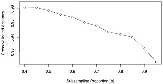
Figure 1.
Cross-validated accuracy against subsampling proportion based on the Wine dataset (averaged over 100 iterations).
As revealed by Figure 1, reducing the subsampling rate offers a direct means to enhance the diversity and improve the predictive performance. Nevertheless, this approach inherently deteriorates the training sample size, which negatively impacts the prediction outcomes. To circumvent this trade-off, we propose two novel subsampling schemes designed to generate a more diverse set of subsamples without compromising their size. Our objective is to foster enhanced diversity among training samples while preserving their scale, thereby further augmenting the performance of subsampling-based ensembles.
2.2. Proposed Methods
In this section, we describe two novel subsampling schemes devised to maximize the diversity among training samples for subsampling-based ensemble methods, thereby enhancing predictive performance without sacrificing training sample size. Before detailing these proposed methods, we will outline some general notation, review the conventional random subsampling approach, and provide additional motivation of our developed methods.
Let B be the total number of subsamples, each of size k (). In subbagging, B also corresponds to the number of individual trees of the ensemble. The traditional approach generates these training samples through random subsampling, drawing k instances from the n observations in a learning dataset without replacement and repeating this process B times independently. In contrast to this conventional approach, we will next discuss our two developed schemes: partition subsampling and shift subsampling.
Inspired by the success and broad applications of the previous work [23,24,25,26], where partition or shift subsampling schemes have proven to be efficient and effective for U-statistic variance estimation [27,28] in applications ranging from cross validation and model comparison and selection to the assessment of AUC (area under ROC curve). The potential of these schemes to improve the diversity within subsampling-based ensembles motivated our research.
2.2.1. Partition Subsampling
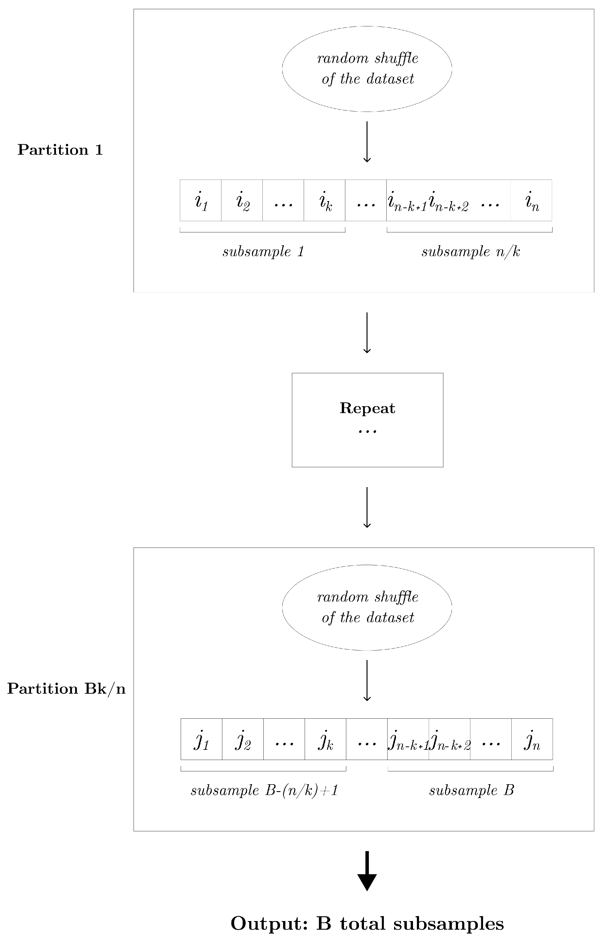
Without loss of generality, assume n is divisible by k. The partition subsampling is applicable whenever the subsampling proportion . It can be realized as follows: We begin by randomly shuffling the given learning sample of size n. This shuffled dataset is then systematically partitioned into disjoint subsamples, each of size k. This process is repeated times to obtain a total of B subsamples. Given a random partition, the generated data subsets are inherently mutually exclusive, thereby maximizing the diversity among them. Furthermore, the partition subsampling scheme guarantees a minimal number of non-overlapping subsamples (i.e., training samples) within an ensemble. Algorithm 1 outlines the detailed procedure, and Figure 2 displays the diagram of the partition subsampling scheme.
| Algorithm 1 Partition Subsampling. |
|

Figure 2.
Diagram that displays the partition subsampling scheme that generates B subsamples of size k.
Remark 1.
The assumption that n is divisible by k is set primarily for notational simplicity, and the algorithm can be easily modified to account for cases where this condition is not met. Let and represent the floor and ceiling of a real number, respectively. When this assumption does not hold, we partition each given learning sample of size n into subsamples of size k. This process is repeated times. In the final random partition, fewer than subsamples may be selected to obtain total of B subsamples.
2.2.2. Shift Subsampling
When the subsampling proportion p is greater than , the partition subsampling scheme is no longer applicable. To address this, we propose an alternative shift subsampling scheme that works effectively for larger subsampling rates. Shift subsampling generates pairs of subsamples, each of size k, with the minimal number of overlaps. Specifically, from a randomly shuffled learning dataset, we extract the first k instances and the last k instances to form a pair of subsamples. This pairing results in overlaps, which is the smallest possible number of between-subsample overlaps in this context. This process is repeated times to yield a total of B subsamples. Note that when , the partition subsampling and shift subsampling are identical. Algorithm 2 describes this procedure in detail, and Figure 3 displays the diagram of the shift subsampling scheme.
| Algorithm 2 Shift Subsampling. |
|
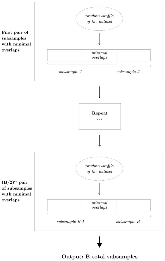
Figure 3.
Diagram that displays the shift subsampling scheme that generates B subsamples of size k.
Shift subsampling is particularly effective when the training sample size k is relatively large (). In this context, random subsampling is more likely to generate data subsets with a significant amount of overlap. Shift subsampling is designed to maximize diversity between training datasets, making it a valuable scheme for larger sample sizes. Using a larger training sample size is generally desirable, as it often leads to more accurate individual predictions. Therefore, from this aspect, shift subsampling is expected to yield more accurate results than partition subsampling, which is limited to scenarios. These inherent design features—maximizing the diversity and utilizing larger sample sizes—explain the advantage and success of shift subsampling over other methods, as demonstrated in the numerical studies in Section 3.
Remark 2.
For random subsampling, the cost of the most efficient algorithm that generates a subsample of size is . Thus, creating B subsamples requires a total cost of . In comparison, for partition subsampling, an initial random shuffle of the dataset of size n demands an effort, which yields subsamples. Thus, under partition subsampling, the total cost for generating B subsamples is , which simplifies to . Similarly, shift subsampling also starts with an shuffle but produces only two subsamples. Therefore, generating B subsamples demands a computational effort of order , where, by design, in the context of shift subsampling. Overall, the computational costs of partition subsampling, shift subsampling, and the benchmark random subsampling are all comparable.
2.2.3. Probabilistic Investigation
As the two proposed subsampling schemes entail, each of them aim to maximize diversity among training datasets. To further justify their superiority over the conventional random subsampling, we take a probabilistic approach to measure their diversity by focusing on between-subample overlaps.
Given a subsampling strategy, let X be the number of overlaps between two randomly generated subsamples. When , X takes values of , while for . In both scenarios, it is easy to see that, under random subsampling, the probability mass function of X can be written as
where for and for . This agrees with the probability mass function of a Hypergeometric distribution with parameters .
In contrast, under the partition-subsampling scheme (i.e., ), the probability that a pair of generated subsamples have exactly c overlaps can be expressed as follows
Equation (2) can be verified as follows.
Proof.
In the following derivations, we utilize the Law of Total Probability, a fundamental rule in probability theory, to calculate the probability of zero overlaps by considering two mutually exclusive scenarios. In the case of partition subsampling, the pair of subsamples may be drawn from the same partition or may come from two different partitions. Under each of these two conditions, we partition the probability of zero overlaps to complete the derivation. Specifically,
Then, by the General Multiplication Rule in probability theory,
Hence,
Similarly, when , we have
□
Furthermore, under shift subsampling (i.e., ), the probability mass function of X is given by
for .
The proof of Equation (3) is presented below.
Proof.
In the case of shift subsampling, a pair of subsamples may be drawn from the same shuffled dataset or may come from two different shuffled datasets. Under each of these two conditions, we partition the probability of minimal overlaps to complete the derivation. By applying the Law of Total Probability and the General Multiplication Rule in probability theory, when , i.e., the minimal number of overlaps, we have
Similarly, when ,
□
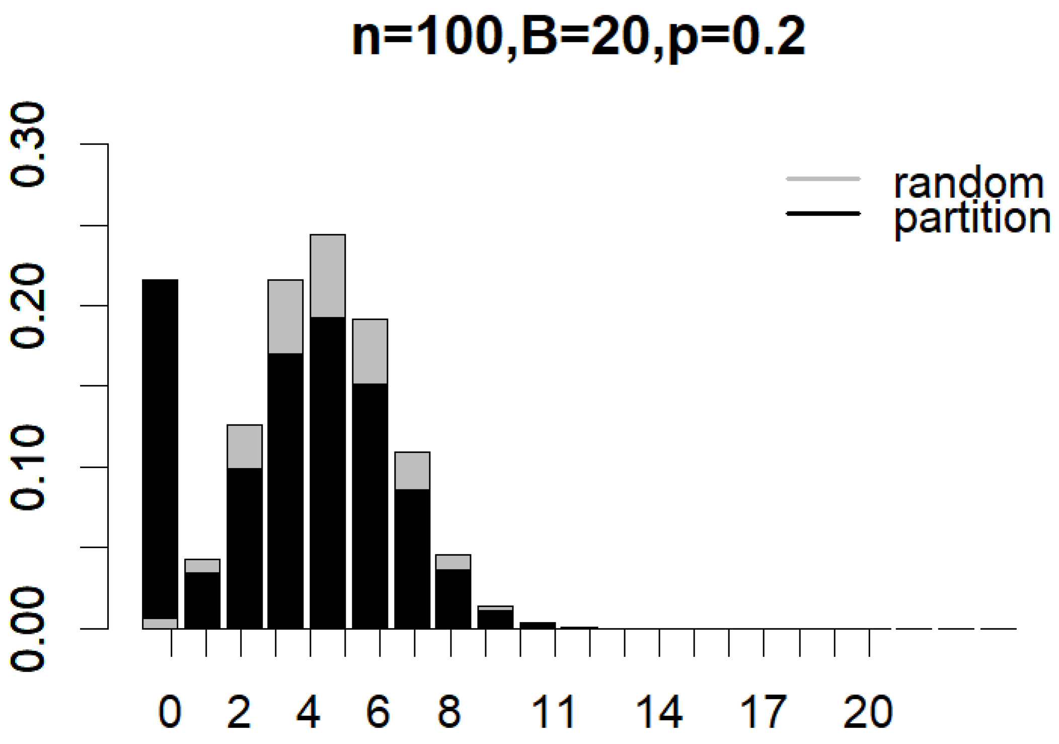
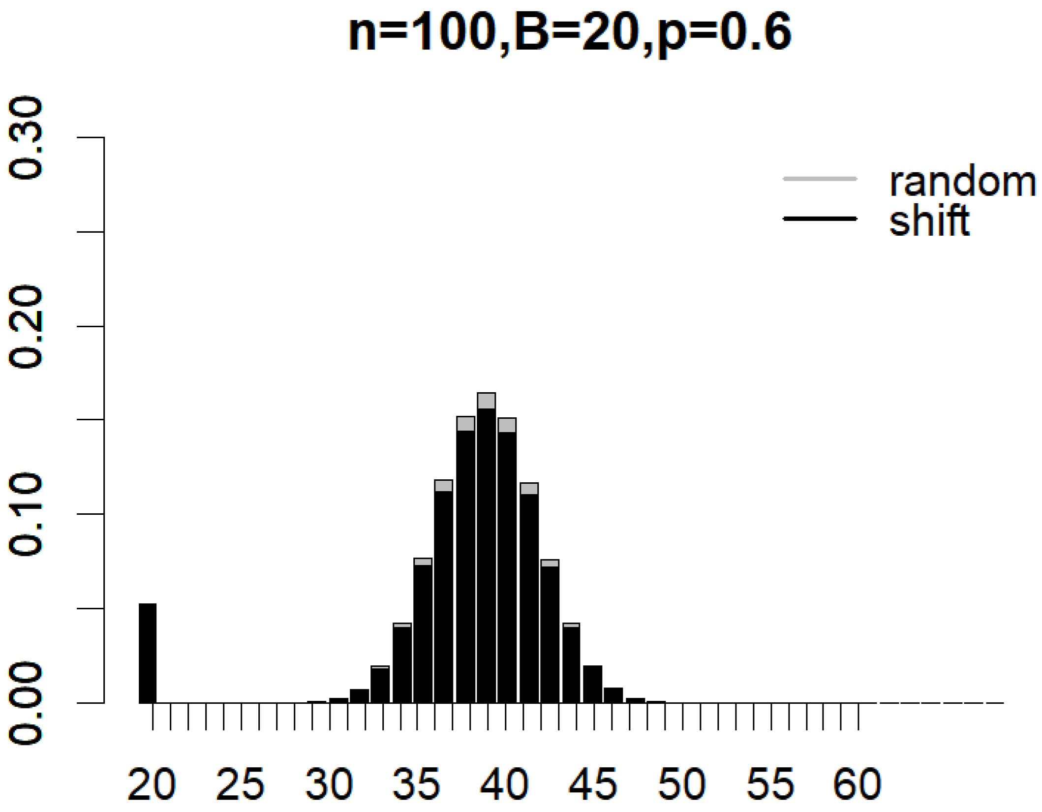
Figure 4 and Figure 5 illustrate the probability mass functions (PMF) under various subsampling schemes, with parameters set to , , and for partition subsampling and for shift subsampling. The two PMFs are shown as overlapping bar charts, with the shorter bars positioned in front. In Figure 4, the first black bar for partition subsampling that corresponds to the probability of generating a non-overlapped pair of subsamples () is so much taller than that under random subsampling (see the first gray bar). In Figure 5, the first black bar for shift subsampling that displays the probability of generating a pair of subsamplings with overlaps (i.e., the minimal overlap) is, once again, much taller than that under random subsampling (in this case, the gray bar has a height that is almost equal to zero). These plots clearly demonstrate how the proposed subsampling designs significantly boost the likelihood of achieving the minimal number of overlaps between subsamples compared to simple random subsampling. As indicated by Equations (1)–(3), the exact reduction in between-subsample overlaps is dependent on n, B, and p. Nevertheless, the clear benefit of incorporating partition and shift subsampling to enhance training sample diversity is evident.
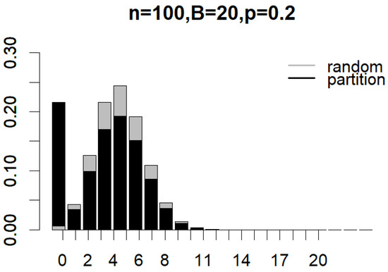
Figure 4.
Probability mass functions of expected overlaps between a pair of subsamples generated from random subsampling and partition subsampling when , , and .
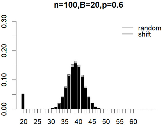
Figure 5.
Probability mass functions of expected overlaps between a pair of subsamples generated from random subsampling and partition subsampling when , , and .
From the probabilistic point of view, there are two possible ways that we may quantify and compare the diversity resulting from various subsampling schemes through a probabilistic perspective: 1. comparing the probability that each method achieves the minimal number of overlaps between a pair of randomly generated subsamples and 2. comparing the expected number of overlaps between a pair of subsamples given a subsampling scheme. Specifically, Table 1 summarizes the comparison for the probability of attaining maximum diversity (i.e., minimum overlaps) among the three subsampling methods.

Table 1.
Comparison of the probability of maximum diversity under a subsampling scheme.
Furthermore, the expected number of overlaps between a pair of subsamples generated from a specific subsampling scheme can be expressed as
where the formula for depends on the subsampling method. Table 2 compares the expected number of overlaps between a pair of random subsamples under different subsampling schemes when , and , or 100. Partition and shift subsampling consistently produce fewer expected overlaps. However, this advantage diminishes as either the sample size n or the ensemble size B increases.

Table 2.
Expected number of overlaps between a pair of subsamples.
In the following section, we conduct comprehensive simulation studies to numerically assess the performance of the proposed subsampling schemes against the benchmark in both classification and regression contexts.
Remark 3.
Because both of our proposed subsampling methods begin with a random shuffle of the entire learning sample, they are best suited for data where the observations are independently and identically distributed. We acknowledge that this approach may inadvertently distort inherent structures within datasets that have complex stratification or strong temporal dependencies. In such cases, specialized algorithms designed to preserve these data features, such as those that account for stratified or time-series data, may be more appropriate.
3. Results
3.1. Simulation Studies
In this section, we evaluate the performance of the proposed subsampling schemes through simulation studies in regression and classification scenarios. For both designs, we consider subsampling rates from to , incremented by . We use the proposed partition subsampling scheme to generate individual training samples for the ensemble when , and the developed shift subsampling scheme for . For comparison purposes, we also realize the conventional random subsampling approach as a benchmark for subsampling-based ensemble methods. We fit individual trees within an ensemble using the randomForest package in R [29]. Each tree was grown to its maximum possible depth until a stopping criterion, such as a minimal mean squared error for regression, was met. The same tree-fitting algorithm was used in both Section 3.1 and Section 3.2.
3.1.1. Classification Simulation Study
For the classification simulation study, we generated independent samples of size n, with . Within each simulated dataset, six x-variables, each of length n, were independently drawn from a standard Uniform distribution. Subsequently, n random errors were simulated from a Logistic distribution with a location parameter of 0 and a scale parameter of 5. The “continuous” response, , was then determined based on the following true relationship:
The binary outcome Y was obtained by dichotomizing the continuous response based on a varying threshold. This threshold was chosen to yield a target ratio of 1’s to 0’s of 50-50, 40-60, 30-70, or 20-80 in the final dataset. Specifically, the threshold was set to be the qth percentile () of the Logistic distribution with a location parameter of 8.05 and a scale parameter of 2, which represents the expected distribution of conditional on the x-variables. A value of greater than the threshold resulted in ; otherwise, . We deliberately included as an irrelevant predictor to introduce noise and elevate the classification task’s difficulty.
For each simulated dataset, we applied the subbagging estimator, varying the number of trees within each ensemble to 50, 100, and 500. As previously mentioned, we also explored a wide range of subsampling rates, from to , with an increment of 0.05. This resulted in subsampling sizes ranging from to . We fit the benchmark subbagging estimator, which uses the default random subsampling scheme, alongside those constructed using our developed partition or shift subsampling strategies. Their performance was compared using a 10-fold cross-validated accuracy measure. The average cross-validated accuracy scores across the 500 iterations are summarized in Table 3, Table 4, Table 5, Table 6, Table 7, Table 8, Table 9 and Table 10. It is worth mentioning that, in Table 6, the values for the smallest subsampling proportion () are marked as NA. This occurred because, at such a low subsampling rate and given the imblanced nature of the simulated dataset, it is probable to have only 0 s in some training sets through 10-fold cross validation, making it impossible to fit the model. (For example, when n = 100 and , a 10-fold cross validation results in training sets with only nine observations each for the ensemble. Given a 20-80 positive–negative ratio, it is highly likely that some of these small training samples will contain no positive cases (1’s) due to random chance).

Table 3.
Cross-validated accuracies in binary classification when and a 50-50 positive–negative ratio.

Table 4.
Cross-validated accuracies in binary classification when and a 40-60 positive–negative ratio.

Table 5.
Cross-validated accuracies in binary classification when and a 30-70 positive–negative ratio.

Table 6.
Cross-validated accuracies in binary classification when and a 20-80 positive–negative ratio.

Table 7.
Cross-validated accuracies in binary classification when and a 50-50 positive–negative ratio.

Table 8.
Cross-validated accuracies in binary classification when and a 40-60 positive–negative ratio.

Table 9.
Cross-validated accuracies in binary classification when and a 30-70 positive–negative ratio.

Table 10.
Cross-validated accuracies in binary classification when and a 20-80 positive–negative ratio.
The simulation results further confirmed the role of diversity on the ensemble predictive performance: across all three subsampling methods, as the subsampling rate increases—reducing diversity among individual training samples—the accuracy consistently deteriorates. This pattern holds true for both sample sizes. On the other hand, as the sample size n increases from 100 to 500, or the number of trees per ensemble becomes larger, there is a slight improvement in accuracy scores across various subsampling rates, given the same positive–negative ratio.
The proposed subsampling schemes demonstrate superior predictive performance as the subsampling rate increases. Notably, the performance gains from our methods become apparent at relatively small subsampling rates, particularly with larger sample sizes. For example, when and a 50-50 positive–negative ratio, the partition subsampling scheme starts to outperform the benchmark at approximately . This threshold drops to around for . Overall, the proposed methods ultimately achieve a higher accuracy than the benchmark beyond a certain threshold. An additional notable observation is that the shift subsampling yields a more significant improvement in accuracy. For example, in Table 3, shift subsampling with boosts the benchmark’s accuracy by up to (see Table 3 when and #trees : the improvement in accuracy is ), whereas the partition subsampling (e.g., at to ) only improves the accuracy by 1–2%.
3.1.2. Regression Simulation Study
For the regression simulation study, we used a Multivariate Adaptive Regression Spline (MARS) model, also known as Friedman #1 [30]. This model allows the generation of datasets that exhibit an underlying non-linear relationship between the response and five predictor variables. It is a common benchmark for evaluating ensemble methods and has been considered in several previous studies, including Bühlmann and Yu [10], Mentch and Hooker [11], Wang and Wei [13]. For each sample of size n (either 100 or 500), we independently simulated five x-variables from a standard Uniform distribution. Random errors were then generated from a normal distribution with a mean of 0 and a standard deviation of or . The response was then determined based on the following relationship:
In total, we considered independent samples.
Similar to the classification study, we applied the subbagging estimator with varying numbers of trees—specifically, 50, 100, and 500 per ensemble. We also explored a wide range of subsampling rates, from to , increasing by 0.05. We fit both the benchmark subbagging estimator (using the default random subsampling scheme) and those developed with our partition or shift subsampling strategies. To compare their performance, we computed the 10-fold cross-validated mean squared error (MSE). The average cross-validated MSEs from the 500 iterations are summarized in Table 11, Table 12, Table 13, Table 14, Table 15 and Table 16.

Table 11.
Cross-validated mean squared error (MSE) in regression when and error standard deviation .

Table 12.
Cross-validated mean squared error (MSE) in regression when and error standard deviation .

Table 13.
Cross-validated mean squared error (MSE) in regression when and error standard deviation .

Table 14.
Cross-validated mean squared error (MSE) in regression when and error standard deviation .

Table 15.
Cross-validated mean squared error (MSE) in regression when and error standard deviation .

Table 16.
Cross-validated mean squared error (MSE) in regression when and error standard deviation .
The simulation results for the regression show a slightly different pattern than those observed in the classification scenario. For random subsampling, the MSE initially decreases with the subsampling rate but then increases. In contrast, under partition and shift subsampling, the MSE decreases monotonously with a larger subsampling rate. This ultimately leads to a much reduced MSE under shift subsampling at , with an up to 37% reduction in MSE compared to the benchmark (see Table 14 for the specific case where and the number of trees is 500. This value was obtained from the calculation: , namely, a 37% reduction in MSE). In addition, as expected, we found that increasing the number of trees or decreasing the error standard deviation slightly reduces the MSE. This pattern holds true for both sample sizes. Furthermore, a larger sample size consistently leads to better overall performance, resulting in a lower MSE. From a different aspect, the threshold for observing superior performance from our proposed methods is lower when the error standard deviation increases or when the number of trees increases.
3.2. Real Data Examples
In this section, we present eight real data examples to demonstrate the practical applications of the proposed subsampling schemes compared to the benchmark random subsampling in both the regression and classification scenarios.
3.2.1. Classification Datasets
We first evaluated our proposed methods and the benchmark using five diverse classification datasets, each presenting unique characteristics in terms of the sample size, number of features, class distribution, and application domains. In addition to the Wine dataset [22] discussed in Section 2.1, we also considered several other classification datasets. More specifically, the Iris dataset [31], one of the earliest known datasets used to evaluate classification methods, includes 150 observations. It uses four continuous variables (petal and sepal length and width) to predict one of three balanced iris plant species. In addition, we utilized the Cleveland database for heart disease diagnosis [32]. This dataset has 300 observations and contains information on thirteen demographic and health-related variables to predict one of five heart disease severity levels (0–4, where 0 indicates no disease). We also analyzed the Pima Indians Diabetes dataset [33], comprising 760 observations with eight health-related variables to predict diabetes presence (i.e., binary outcome). Lastly, the Statlog (German Credit Data) dataset [34] contains 1000 observations and classifies individuals as good or bad credit risks based on 20 financial and demographic features. All the aforementioned datasets are available in the UCI Machine Learning Repository (https://archive.ics.uci.edu/).
Table 17 summarizes the characteristics of these datasets. For ease of implementation of 10-fold cross validation, we round the number of observations down to a multiple of 10 by randomly removing fewer than 10 observations from each dataset. All reported sample sizes reflect these adjusted counts.

Table 17.
Classification dataset quantitative summary.
We applied subbagging estimators by varying the number of trees per ensemble from 20 to 1000. For each of the five datasets, we generated subsamples for individual classification trees using two methods: random subsampling (the benchmark) and shift and partition subsampling (our proposed methods). Moreoever, we set the subsampling proportion p from 0.1 to 0.95, incrementally increasing by 0.05. This resulted in subsample sizes k ranging from to . Consistent with our approach in Section 2.1, we assessed the performance of each method using 10-fold cross-validated accuracy scores for each dataset and setting. To mitigate the impact of randomness inherent in ensemble learning, we refit the subbagging estimator 100 times, reporting the average cross-validated accuracy scores. The results are summarized in Table 18, Table 19, Table 20, Table 21 and Table 22.

Table 18.
Cross-validated accuracy scores based on the Wine dataset.

Table 19.
Cross-validated accuracy scores based on the Iris dataset.

Table 20.
Cross-validated accuracy scores based on the Cleveland dataset.

Table 21.
Cross-validated accuracy scores based on the Diabetes dataset.

Table 22.
Cross-validated accuracy scores based on the German dataset.
Across all five classification datasets, the accuracy generally declines with the subsampling rate past a certain inflection point. This trend is most noticeable with random subsampling, which leads to a significant drop in accuracy at . In contrast, partition and shift subsampling enable higher subsampling rates to improve the accuracy. For example, shift subsampling on the Wine dataset achieves an accuracy of nearly or above 96%, representing an improvement of up to 5% over the benchmark. Further, the improvement of shift subsampling reaches 10% on the German dataset. Consistent with our findings in Section 3.1, the accuracy also improves with a larger ensemble size and a more balanced class ratio.
3.2.2. Regression Datasets
To further demonstrate the performance of the developed methods in a different setting, we considered three real-world regression datasets. First, we analyzed the Housing dataset [35], which predicts house price per unit area for properties in Xindian District, New Taipei City, Taiwan, using six features. Next, we utilized the Energy Efficiency dataset [36], which assesses building energy efficiency based on eight building parameters. Finally, we incorporated the Forest Fires dataset [37]. This dataset attempts to predict the burned area of forest fires in the northeast region of Portugal using twelve meteorological features. Following the documentation and the prior literature [38], a natural logarithm transformation was applied to the highly skewed response variable. One thing worthy of attention is that the Forest Fires dataset is particularly challenging to model. Previous attempts to analyze it using machine learning techniques have not been very successful [38].
Table 23 presents the summary characteristics of these datasets. Similar to our previous approach, we rounded the number of observations down to a multiple of 10 by randomly removing fewer than 10 observations to simplify the 10-fold cross validation. All the sample sizes reported in Table 23 are after these adjustments.

Table 23.
Regression dataset quantitative summary.
Using the three aforementioned datasets, we examined the performance of different subbagging estimator configurations, evaluating each based on the cross-validated mean squared error (MSE). Consistent with the settings in Section 3.2.1, we varied the subsampling proportion p from 0.10 to 0.95 and the number of trees per ensemble from 20 to 1000. All MSE scores were computed using 10-fold cross validation. The complete results are summarized in Table 24, Table 25 and Table 26.

Table 24.
Cross-validated MSEs based on the Housing dataset.

Table 25.
Cross-validated MSEs based on the Energy dataset.

Table 26.
Cross-validated MSEs based on the Forest Fires dataset.
Under random subsampling, a different inflection point of MSE is observed for each dataset. Specifically, in the Housing dataset, the MSE initially decreases as the subsampling proportion (p) increases from 0.10 to 0.40 and then begins to rise for p values between 0.40 and 0.95. Conversely, the Forest Fires dataset consistently shows an increase in the MSE with larger subsampling proportions. For the Energy dataset, however, increased subsampling proportions lead to lower errors. Similarly, distinct trends in the prediction error (MSE) are also observed when utilizing partition or shift subsampling. Specifically, under the proposed subsampling schemes: In the Housing dataset, the MSE decreases as the subsampling proportion (p) increases from approximately 0.10 to 0.60 and then rises from roughly 0.60 to 0.95. For the Energy dataset, increased subsampling proportions generally yield lower errors. On the contrary, in the Forest Fires dataset, higher subsampling proportions are associated with increased errors. Across all three datasets, as the number of trees per ensemble increases, we observe a general trend of decreasing MSE. This reduction is most pronounced when the number of trees grows from 20 to 100; beyond that point, only marginal further decreases in MSE are observed. This holds true across all different subsampling schemes.
Regarding the comparison between the benchmark and our proposed methods, the benefits of our subsampling scheme become more pronounced when increasing the subsampling proportion. For both the Housing and Energy datasets, our proposed method begins to show improvement at a subsampling proportion of approximately . In contrast, for the challenging Forest Fires dataset, a gain in MSE is consistently observed across all tested values of p, which proves the advantage of our proposed methods for more challenging datasets. Across all datasets, a marginal positive correlation between the number of trees per ensemble and the magnitude of the gain in MSE is also noted.
3.3. Further Justification
As discussed in the previous sections, to mitigate the effects of randomness, we used 500 iterations for each simulation study. For the real data examples, each subbagging estimator was refitted 100 times. The reported performance scores are therefore averages over a large number of iterations, effectively accounting for random variations.
To further demonstrate the superior performance of our proposed subsampling schemes, in what follows, we use the Wine dataset as a case study to better justify the effectiveness and significance of our developed methods compared to the benchmark random subsampling.
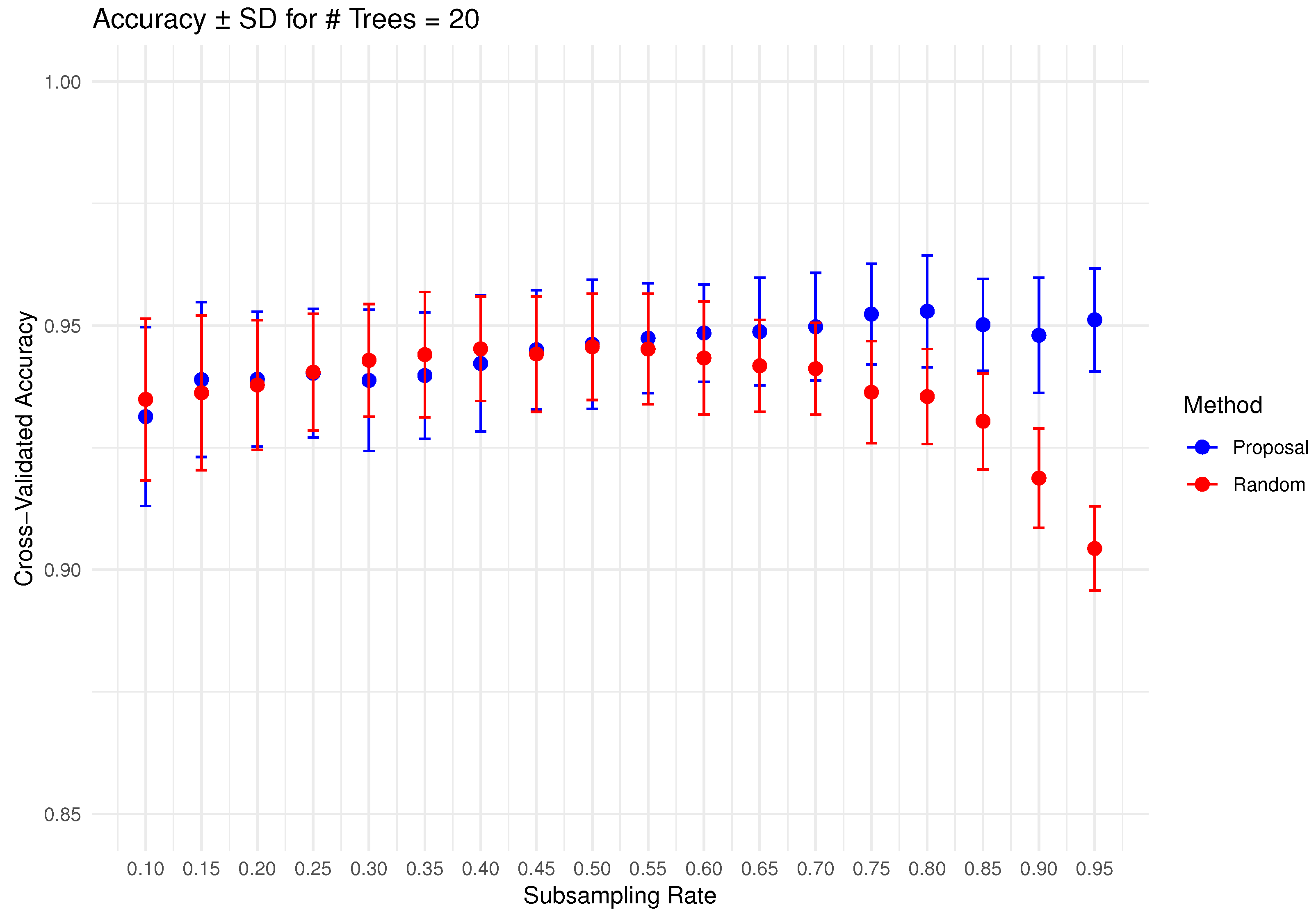
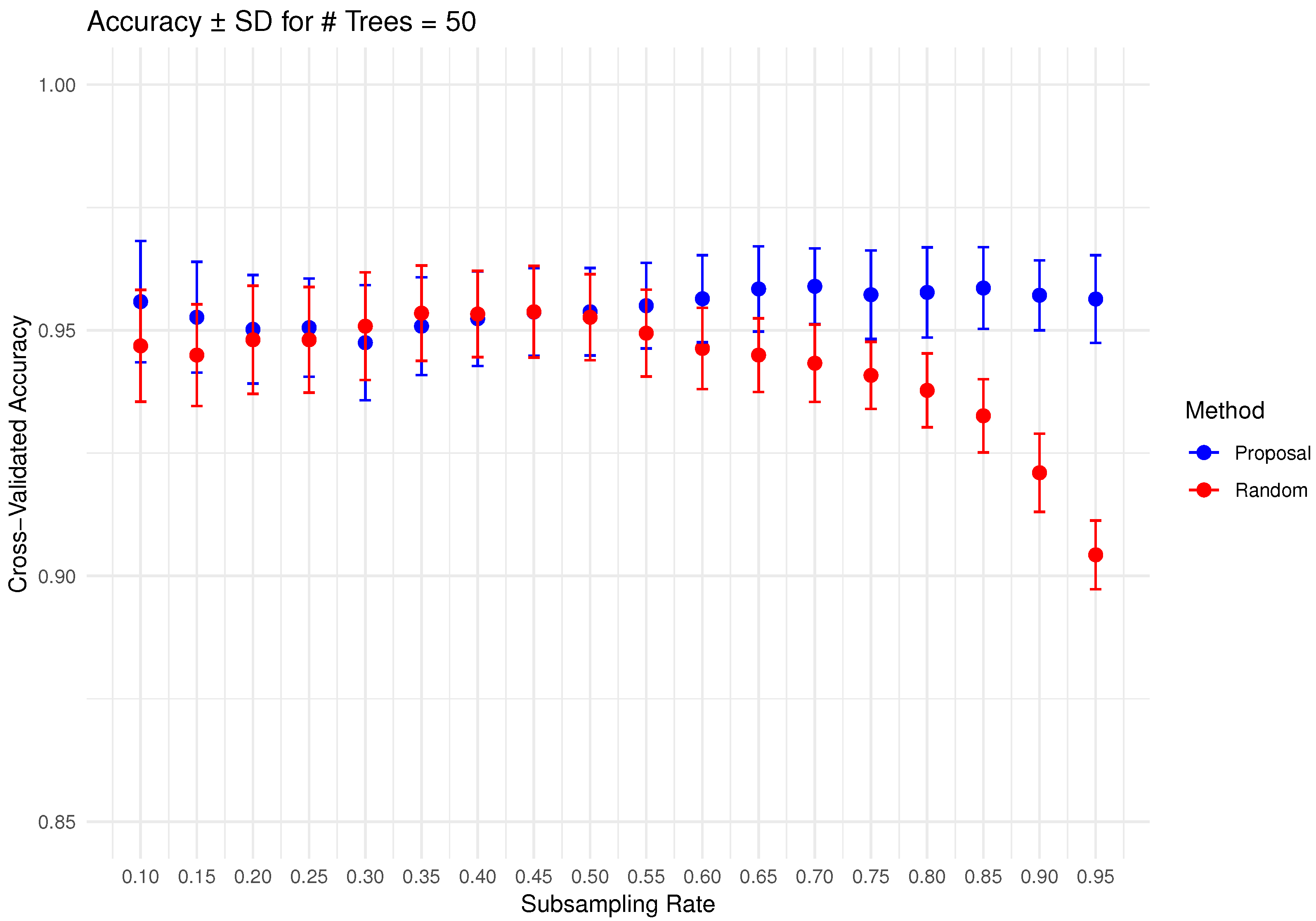
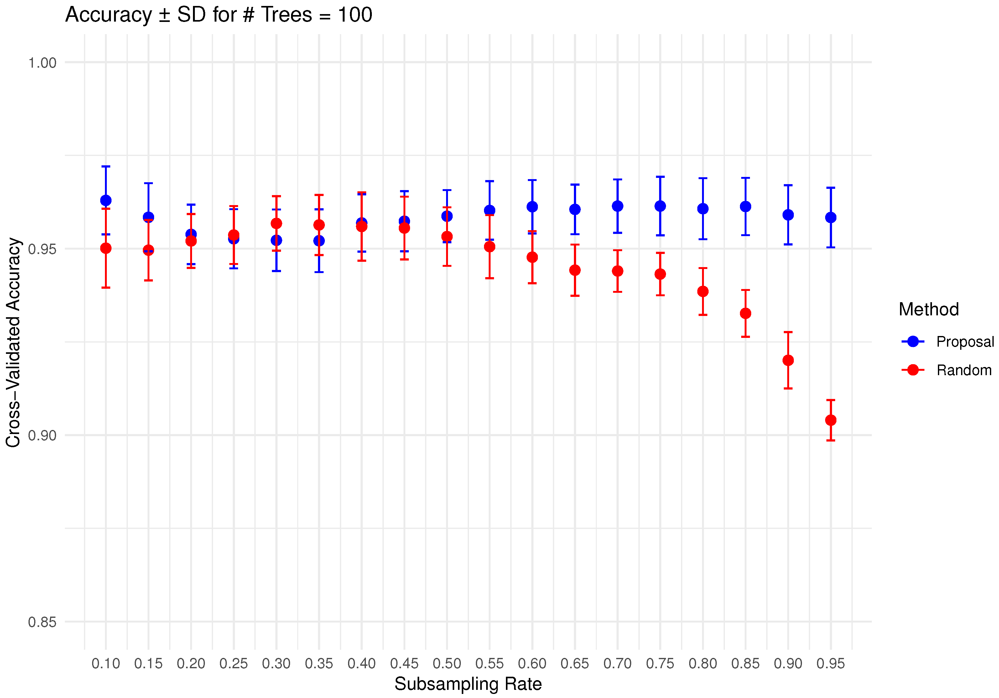
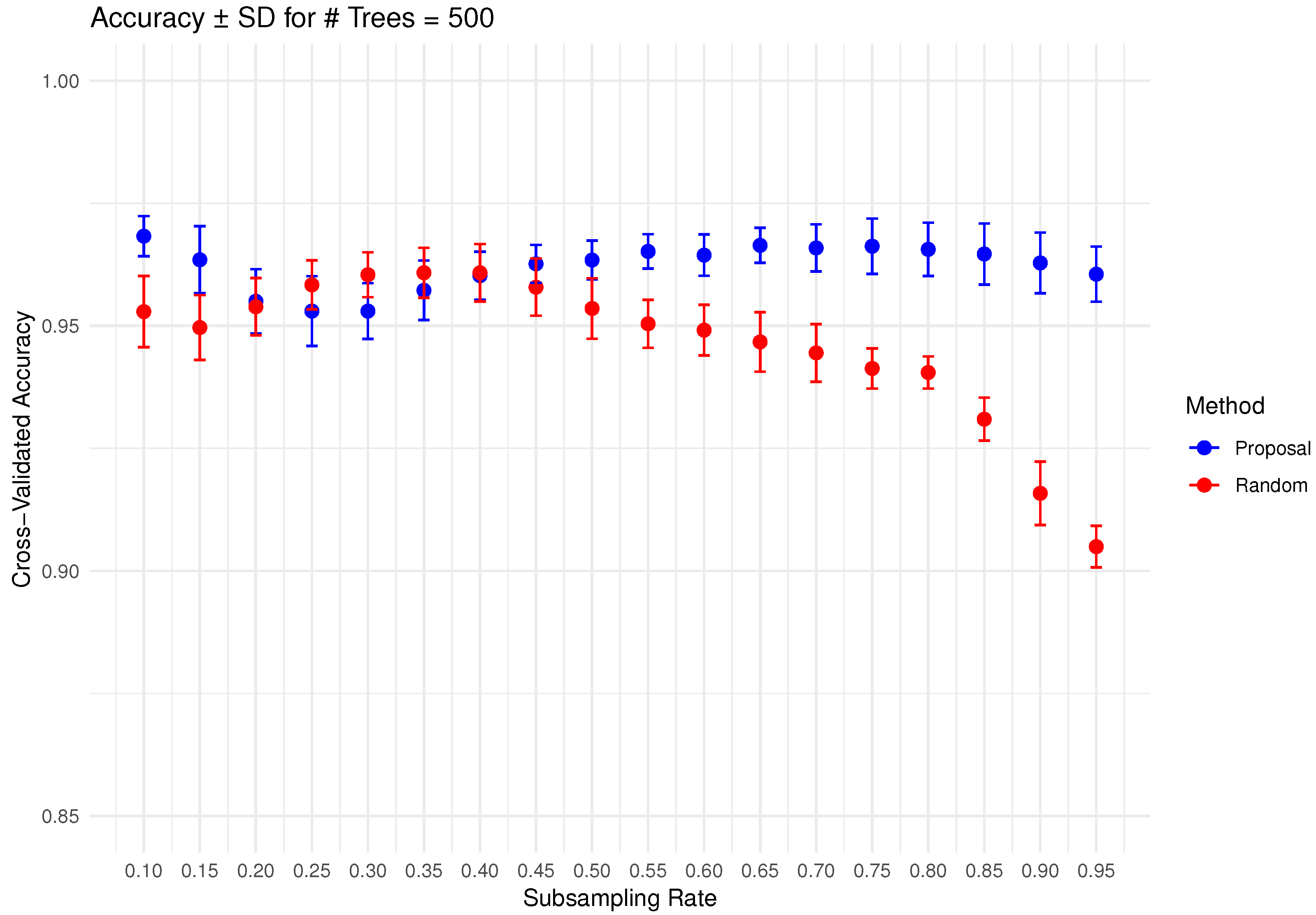
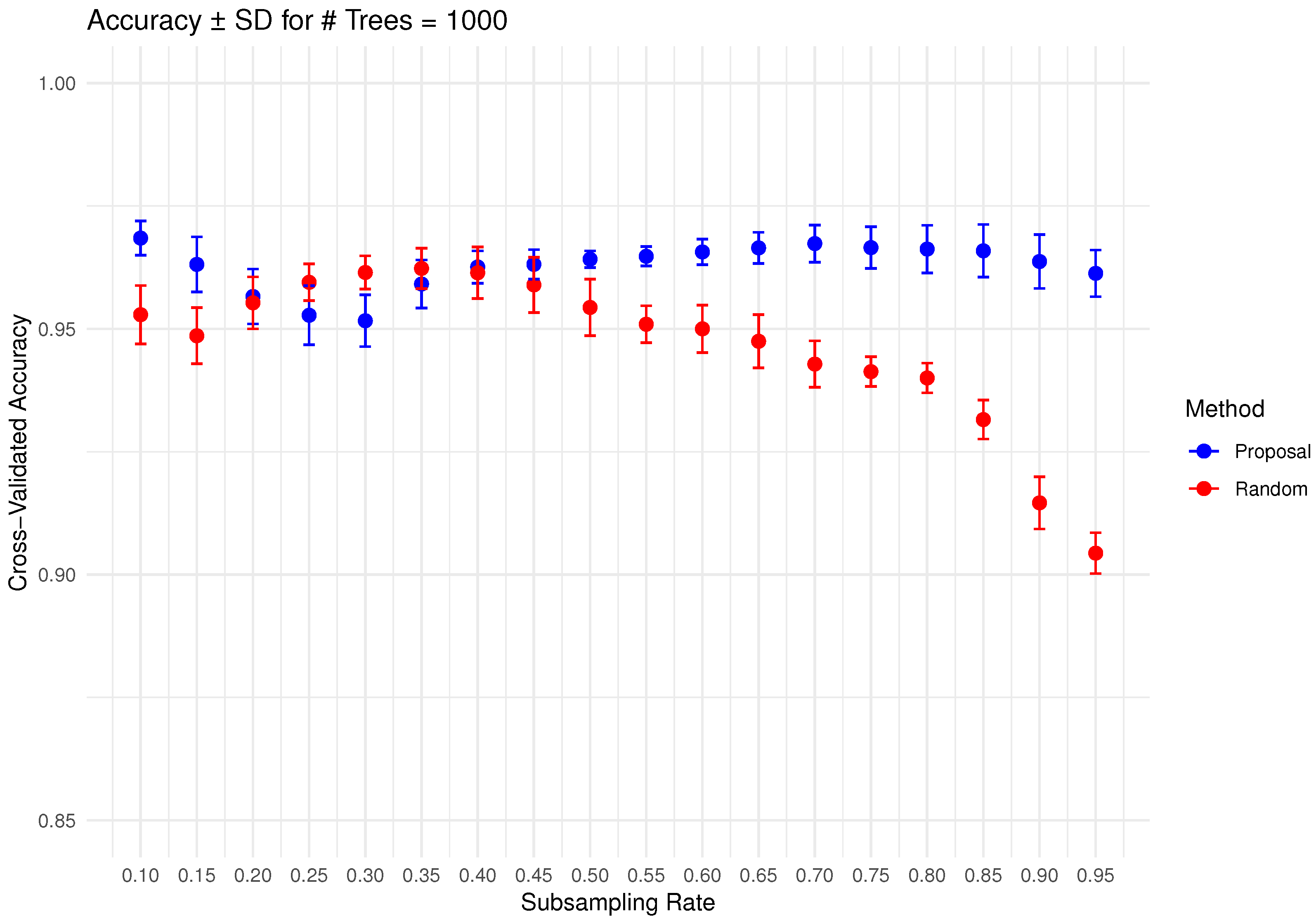
In Figure 6, Figure 7, Figure 8, Figure 9 and Figure 10 below, we display the cross-validated accuracy scores of different methods. The solid dots represent the average score over 100 refits of the subbagging estimator, for a given subsample size and and number of trees. The error bars around each dot indicate the standard error. As anticipated, the standard error of accuracy score decreases as the number of trees increases. These plots show that, on average, our proposed partition and shift subsampling schemes consistently outperform the benchmark random subsampling, with only a few exceptions where their performance scores are quite comparable. This performance gain becomes particularly significant as the subsampling rate and the number of trees increase, even after accounting for sampling variations. As discussed in Section 2.2.2, shift subsampling tends to be particularly advantageous over the other competing methods at relatively large subsampling rates. For example, in Figure 10 when and with 1000 trees per ensemble, shift subsampling is significantly better than the benchmark, yielding a much higher cross-validated accuracy. Overall, the threshold for such significant performance gain appears at a lower subsampling rate when the number of trees grows.
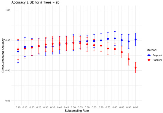
Figure 6.
Cross-validated accuracy with error bars based on the Wine dataset (#trees ).
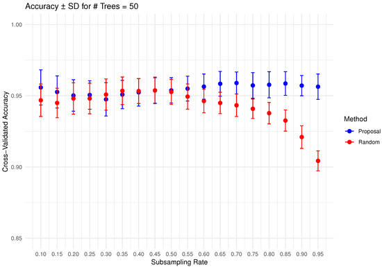
Figure 7.
Cross-validated accuracy with error bars based on the Wine dataset (#trees ).
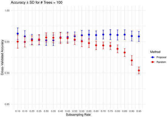
Figure 8.
Cross-validated accuracy with error bars based on the Wine dataset (#trees ).
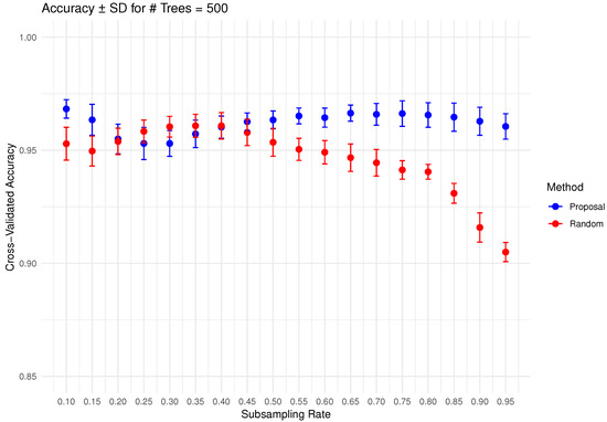
Figure 9.
Cross-validated accuracy with error bars based on the Wine dataset (#trees ).
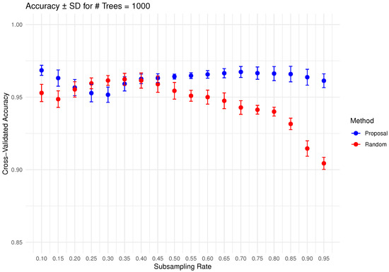
Figure 10.
Cross-validated accuracy with error bars based on the Wine dataset (#trees ).
4. Discussion
This paper explores how diversity among training samples impacts the predictive performance of subsampling-based ensemble methods. To improve the diversity without compromising the training sample size, we introduce two novel subsampling schemes: partition subsampling and shift subsampling. Our probabilistic analyses further justify the improved diversity the proposed methods offer compared to the benchmark random subsampling. Through extensive simulation studies and real-world data illustrations, we show their superior performance in both regression and classification scenarios. In particular, the benefits of utilizing the developed subsampling strategies become more noticeable on challenging datasets or at larger subsampling rates, and the percent of improvement is more significant in regression problems.
For future work, it would be interesting to extend these schemes to other subsampling-based ensemble methods, such as sub-random forest or non-tree-based sub-ensemble estimators. Given their adaptability, we anticipate similar positive trends and conclusions in these broader applications.
Author Contributions
Conceptualization, Q.W.; methodology, M.O. and Q.W.; software, M.O. and Q.W.; validation, M.O. and Q.W.; formal analysis, M.O. and Q.W.; investigation, M.O. and Q.W.; resources, M.O.; data curation, M.O.; writing—original draft preparation, M.O. and Q.W.; writing—review and editing, M.O. and Q.W.; visualization, M.O. and Q.W.; supervision, Q.W. All authors have read and agreed to the published version of the manuscript.
Funding
This research received no external funding.
Data Availability Statement
All the real datasets presented in this paper are available in the UCI Machine Learning Repository (https://archive.ics.uci.edu/).
Acknowledgments
The publication fees for this article are supported by the Wellesley College Library and Technology Services Open Access Fund.
Conflicts of Interest
The authors declare no conflicts of interest.
References
- Galton, F. Regression Towards Mediocrity in Hereditary Stature. J. Anthropol. Inst. Great Br. Irel. 1886, 15, 246–263. [Google Scholar] [CrossRef]
- Heckman, N.; Ramsay, J. Penalized Regression with Model-Based Penalties. Can. J. Stat. 2000, 28, 241–258. [Google Scholar] [CrossRef]
- Dobson, A.; Barnett, A. An Introduction to Generalized Linear Models, 4th ed.; Chapman and Hall/CRC: Boca Raton, FL, USA, 2018. [Google Scholar]
- Gurney, K. An Introduction to Neural Networks; CRC Press: London, UK, 2018. [Google Scholar]
- Zhou, Y.; Gallins, P. A Review and Tutorial of Machine Learning Methods for Microbiome Host Trait Prediction. Front. Genet. 2019, 10, 579. [Google Scholar] [CrossRef] [PubMed]
- Schoot, R.v.; Depaoli, S.; King, R.; Kramer, B.; Märtens, K.; Tadesse, M.G.; Vannucci, M.; Gelman, A.; Veen, D.; Willemsen, J.; et al. Bayesian statistics and modelling. Nat. Rev. Methods Prim. 2021, 1, 1. [Google Scholar] [CrossRef]
- Breiman, L.; Friedman, J.; Stone, C.J.; Olshen, R.A. Classification and Regression Trees; Taylor and Francis: New York, NY, USA, 1984. [Google Scholar]
- Breiman, L. Bagging Predictors. Mach. Learn. 1996, 24, 123–140. [Google Scholar] [CrossRef]
- Breiman, L. Random Forests. Mach. Learn. 2001, 45, 5–32. [Google Scholar] [CrossRef]
- Bühlmann, P.; Yu, B. Analyzing bagging. Ann. Stat. 2002, 30, 927–961. [Google Scholar] [CrossRef]
- Mentch, L.; Hooker, G. Quantifying uncertainty in random forest via confidence intervals and hypothesis tests. J. Mach. Learn. Res. 2016, 17, 1–41. [Google Scholar]
- Peng, W.; Coleman, T.; Mentch, L. Rates of convergence for random forests via generalized U-statistics. Electron. J. Stat. 2022, 16, 232–292. [Google Scholar] [CrossRef]
- Wang, Q.; Wei, Y. Quantifying uncertainty of subsampling-based ensemble methods under a U-statistic framework. J. Statisitcal Comput. Simul. 2022, 92, 3706–3726. [Google Scholar] [CrossRef]
- Kuncheva, L.; Whitaker, C. Measures of Diversity in Classifier Ensembles and Their Relationship with the Ensemble Accuracy. Mach. Learn. 2003, 51, 181–207. [Google Scholar] [CrossRef]
- Brown, G.; Wyatt, J.; Harris, R.; Yao, X. Diversity creation methods: A survey and categorisation. Inf. Fusion 2005, 6, 5–20. [Google Scholar] [CrossRef]
- Kuncheva, L. Combining Pattern Classifiers: Methods and Algorithms; Wiley: Hoboken, NJ, USA, 2004. [Google Scholar]
- Rodríguez, J.J.; Kuncheva, L.I.; Alonso, C.J. Rotation Forest: A new classifier ensemble method. IEEE Trans. Pattern Anal. Mach. Intell. 2006, 28, 1619–1630. [Google Scholar] [CrossRef]
- Freund, Y.; Schapire, R.E. A decision-theoretic generalization of on-line learning and an application to boosting. J. Comput. Syst. Sci. 1997, 55, 119–139. [Google Scholar] [CrossRef]
- Cunningham, P. Ensembles in Machine Learning. 2022. Available online: https://medium.com/data-science/ensembles-in-machine-learning-9128215629d1 (accessed on 15 August 2025).
- Tang, E.K.; Suganthan, P.N.; Yao, X. An analysis of diversity measures. Mach. Learn. 2006, 65, 247–271. [Google Scholar] [CrossRef]
- Wood, D.; Mu, T.; Webb, A.; Reeve, H.W.J.; Lujan, M.; Brown, G. A Unified Theory of Diversity in Ensemble Learning. J. Mach. Learn. Res. 2023, 24, 1–49. [Google Scholar]
- Aeberhard, S.; Forina, M. Wine; UCI Machine Learning Repository: 1991. Available online: https://archive.ics.uci.edu/dataset/109/wine (accessed on 15 August 2025).
- Wang, Q.; Linday, B.G. Variance estimation of a general U-statistic with application to cross-validation. Stat. Sin. 2014, 24, 1117–1141. [Google Scholar]
- Wang, Q.; Guo, A. An efficient variance estimator of AUC with applications to binary classification. Stat. Med. 2020, 39, 4281–4300. [Google Scholar] [CrossRef]
- Wang, Q.; Cai, X. An efficient variance estimator for cross-validation under partition-sampling. Statistics 2021, 55, 660–681. [Google Scholar] [CrossRef]
- Wang, Q.; Cai, X. A new perspective on U-statistic variance estimation. Stat 2025, 14, e70070. [Google Scholar] [CrossRef]
- Hoeffding, W. A class of statistics with asymptotically normal distribution. Ann. Math. Stat. 1948, 19, 293–325. [Google Scholar] [CrossRef]
- Lee, A.J. U-Statistics: Theory and Practice; Marcel Dekker: New York, NY, USA, 1990. [Google Scholar]
- Liaw, A.; Wiener, M. Classification and Regression by randomForest. R News 2002, 2, 18–22. [Google Scholar]
- Friedman, J. Multivariate Adaptive Regression Splines. Ann. Stat. 1991, 19, 1–67. [Google Scholar] [CrossRef]
- Fisher, R.A. Iris; UCI Machine Learning Repository: 1936. Available online: https://archive.ics.uci.edu/dataset/53/iris (accessed on 15 August 2025).
- Janosi, A.; Steinbrunn, W.; Pfisterer, M.; Detrano, R. Heart Disease: Cleveland Database; UCI Machine Learning Repository: 1988. Available online: https://archive.ics.uci.edu/dataset/45/heart+disease (accessed on 15 August 2025).
- Turney, P. Pima Indians Diabetes Data Set; UCI Machine Learning Repository: 1990. Available online: https://www.kaggle.com/datasets/uciml/pima-indians-diabetes-database (accessed on 15 August 2025).
- Hofmann, H. Statlog (German Credit Data); UCI Machine Learning Repository: 1994. Available online: https://archive.ics.uci.edu/dataset/144/statlog+german+credit+data (accessed on 15 August 2025).
- Yeh, I. Real Estate Valuation; UCI Machine Learning Repository: 2018. Available online: https://archive.ics.uci.edu/dataset/477/real+estate+valuation+data+set (accessed on 15 August 2025).
- Tsanas, A.; Xifara, A. Energy Efficiency; UCI Machine Learning Repository: 2012. Available online: https://archive.ics.uci.edu/dataset/242/energy+efficiency (accessed on 15 August 2025).
- Cortez, P.; Morais, A. Forest Fires; UCI Machine Learning Repository: 2008. Available online: https://archive.ics.uci.edu/dataset/162/forest+fires (accessed on 15 August 2025).
- Cortez, P.; Morais, A. A Data Mining Approach to Predict Forest Fires using Meteorological Data. In Proceedings of the 13th Portuguese Conference on Artificial Intelligence (EPIA 2007), Guimarães, Portugal, 3–7 December 2007; pp. 512–523. [Google Scholar]
Disclaimer/Publisher’s Note: The statements, opinions and data contained in all publications are solely those of the individual author(s) and contributor(s) and not of MDPI and/or the editor(s). MDPI and/or the editor(s) disclaim responsibility for any injury to people or property resulting from any ideas, methods, instructions or products referred to in the content. |
© 2025 by the authors. Licensee MDPI, Basel, Switzerland. This article is an open access article distributed under the terms and conditions of the Creative Commons Attribution (CC BY) license (https://creativecommons.org/licenses/by/4.0/).


