A Copula-Based Model for Analyzing Bivariate Offense Data

Abstract

We developed a class of bivariate integer-valued time series models using copula theory. Each count time series is modeled as a Markov chain, with serial dependence characterized through copula-based transition probabilities for Poisson and Negative Binomial marginals. Cross-sectional dependence is modeled via a bivariate Gaussian copula, allowing for both positive and negative correlations and providing a flexible dependence structure. Model parameters are estimated using likelihood-based inference, where the bivariate Gaussian copula integral is evaluated through standard randomized Monte Carlo methods. The proposed approach is illustrated through an application to offense data from New South Wales, Australia, demonstrating its effectiveness in capturing complex dependence patterns.

1. Introduction

Multivariate count time series frequently arise in modern statistical analysis and often exhibit dependence both within and between series. In many applications, time-series counts are observed as bivariate vectors that display serial dependence within each series, as well as cross-correlation between the two. Building on the framework of the integer-valued autoregressive moving average model (INARMA), Quoreshi [1] proposed the bivariate integer-valued moving average model (BINMA), which accommodates both positive and negative correlations between counts. He also extended the BINMA model to a multivariate setting. Wang et al. [2] proposed a bivariate zero-inflated Poisson model to analyze occupational injuries. Heinen and Rengifo [3] proposed a multivariate autoregressive conditional doubly Poisson model capable of handling over-dispersion, serial dependence, and cross-correlation. The cross-correlation between the time series was modeled using a multivariate Gaussian copula, and the parameters were estimated through a two-stage procedure. The work of Karlis and Pedeli [4] presented a bivariate integer-valued autoregressive process of order 1 (BINAR (1)) in which the cross-correlation is modeled by the use of copula to accommodate both positive and negative correlations in Poisson and Negative Binomial counts. Also, they illustrated the use of Frank and Gaussian copulas to specify the joint distribution of the innovations. Marginal time series are modeled using Poisson and Negative Binomial INAR(1) models. Ravishanker et al. [5] applied state space models for multivariate count time series and used them to analyze a market dataset. One major advantage of copula-based methods is that they can separate the modeling of marginal and temporal dependence. Bradshaw and Blei [6] constructed a generative model of underreported campus sexual assault data that allows the estimation of the true incidence and reporting rates. Additionally, they used the Hamiltonian Monte Carlo (HMC) sampling scheme for posterior inference regarding reporting rates and assault incidence in each school and applied this method to analyze campus sexual assault data. Cui and Zhu [7] proposed a new bivariate Poisson INGARCH model, which allows for positive or negative cross-correlation between time series. Ahamad et al. [8] proposed a bivariate count data regression model to capture the dependence between multiple crash outcomes that traditional independent count models fail to represent. In this approach, appropriate marginal distributions (such as Poisson or Negative Binomial) are specified for each crash count type, and a copula function is then used to link the two margins to model their joint dependence. Jeng et al. [9] proposed a copula-based time series model to forecast COVID-19 cases and trends based on wastewater SARS-CoV-2 viral load and clinical variables. The model was developed in two stages. In the first stage, time-series methods were used to examine and characterize the marginal distributions of both the dependent and independent variables. In the second stage, copula-based marginal regression analysis was applied to model and predict the COVID-19 case trends.

Traditional bivariate Negative Binomial regression models typically assume a specific joint distribution for the dependent variables or their associated error terms. A common approach is to impose a bivariate gamma distribution on the error terms when combined in the bivariate framework. However, such assumptions may inadequately capture the underlying dependence structure between the error terms. Moreover, as noted by Xu and Hardin [10], there is no explicit joint distribution for the error terms in this setting. This limitation motivates the need for more flexible approaches. In particular, a copula-based bivariate Negative Binomial model provides a natural extension. In this previous work (alaqawba et al. [11]), we developed a class of copula-based models to analyze bivariate count data, where the marginal distributions were specified as Poisson and zero-inflated Poisson (ZIP). However, when analyzing count time series data, over-dispersion is often present. In this manuscript, we extend that framework by incorporating Negative Binomial marginals, which better accommodate over-dispersion. The copula-based approach enables us to model each marginal distribution appropriately while flexibly capturing the dependence between the series through the selected copula family. This flexibility allows the model to accommodate both positive and negative dependence, providing a more general and adaptable framework for analyzing bivariate count time series data.

The remainder of the paper is organized as follows. Section 2 provides a concise overview of Poisson and Negative Binomial regression models, along with a summary of copula theory. It then introduces the proposed class of copula-based bivariate models for analyzing two dependent time series, where each series is modeled through a copula-based Markov chain and jointly linked using a bivariate copula family. Section 3 outlines the parameter estimation procedure via Maximum Likelihood Estimation (MLE), presents the results of simulation studies, and applies the proposed methodology to a real dataset. Finally, Section 4 concludes the paper.

2. Materials and Methods

2.1. The Poisson Distribution

The Poisson distribution is a common choice for modeling count data. In our proposed copula-based bivariate model, we use it as a marginal distribution. Let $y_t$ represent a random count observed at time t. The probability mass function (pmf) of the Poisson distribution is given by:

$$f\left(y_t\right)={\displaystyle \frac{e^{-\lambda }{\lambda }^{y_t}}{y_t!}},$$

where $\lambda >0$ is the intensity parameter with $E\left(y_t\right)=\lambda$ and $V\left(y_t\right)=\lambda$.

2.2. The Negative Binomial Distribution

With the introduction of an additional parameter $\left(\kappa \right)$ the Negative Binomial distribution is able to account for over-dispersion when compared to the Poisson distribution.

$$f\left(y_t\right)={\displaystyle \frac{\Gamma (\kappa +y_t)}{\Gamma \left(\kappa \right)y_t!}}{\left({\displaystyle \frac{\kappa }{\kappa +\lambda }}\right)}^{\kappa }{\left({\displaystyle \frac{\lambda }{\kappa +\lambda }}\right)}^{y_t}for{y}_t=0,1,2,\dots$$

where $\lambda$ and $\kappa$ are parameters associated with intensity and dispersion with $E\left(y_t\right)=\lambda$ and $V\left(y_t\right)=\lambda +{\displaystyle \frac{{\lambda }^2}{\kappa }}$.

2.3. Copulas

As a multivariate cumulative distribution function (cdf), the copula is a joint function that captures the dependence structure between variables. With uniform margins $U(0,1)$ as in Nelson [12], a n-dimensional copula is a function $C:{[0,1]}^n\to [0,1]$ with the following three properties:

• $C(1,\dots ,u_t,\dots ,1)=u_t,\forall t=1,2,\dots ,n$ and $u_t\in [0,1].$
• $C(u_1,u_2,\dots ,u_n)=0$ if at least one $u_t=0$ for $t=1,2,\dots ,n.$
• For any $u_{t_1},u_{t_2}\in [0,1]$ with $u_{t_1}\le u_{t_2}$, for $t=1,2,\dots ,n,$

  $$\sum _{j_1=1}^2\sum _{j_2=1}^2\cdots \sum _{j_n=1}^2{(-1)}^{j_1+j_2+\cdots +j_n}C(u_{1j_1},u_{2j_2}\dots ,u_{n{j}_n})\ge 0.$$

Let $Y_1,\dots ,Y_n$ be r.v.’s with marginal cdf’s $F_1,\dots ,F_n$ and joint cdf F, then

• there exists an n-dimensional copula C such that for all $y_1,\dots ,y_n\in \mathbb{R}$

  $$F(y_1,y_2,\dots ,y_n)=C(F_1\left(y_1\right),F_2\left(y_2\right),\dots ,F_n\left(y_n\right)).$$
• If $Y_1,\dots ,Y_n$ are continuous then the copula C is unique. Otherwise, C can be uniquely determined on n dimensional rectangle $Range\left(F_1\right)\times Range\left(F_2\right)\times \cdots \times Range\left(F_n\right)$.

When all the margins are integer valued, the multivariate probability mass function can be obtained as

$$f(y_1,y_2,\dots ,y_n)=P(Y_1=y_1,Y_2=y_2,\dots ,Y_n=y_n)$$

$$=\sum _{j_1=1}^2\sum _{j_2=1}^2\cdots \sum _{j_n=1}^2{(-1)}^{j_1+j_2+\dots +j_n}C(u_{1j_1},u_{2j_2}\dots ,u_{n{j}_n})$$

(1)

where $u_{t1}=F_t\left(y_t\right)$ and $u_{t2}=F_t\left(y_t^{-}\right)$. Here $F_t\left(y_t^{-}\right)$ is the left-hand limit of $F_t$ at $y_t$, which is equal to $F_t(y_t-1)$. In the bivariate case,

$$\begin{array}{cc}Pr(Y_1=y_1,Y_2=y_2)\hfill & =C(F\left(y_1\right),F\left(y_2\right);\mathit{\theta })-C(F\left(y_1^{-}\right),F\left(y_2\right);\mathit{\theta })\hfill \\ & -C(F\left(y_1\right),F\left(y_2^{-}\right);\mathit{\theta })+C(F\left(y_1^{-}\right),F\left(y_2^{-}\right);\mathit{\theta }).\hfill \end{array}$$

Here, $\mathit{\theta }$ denotes the dependence parameter of the copula function, and a variety of copula families, denoted by C, are available for selection.

Table 1. Bivariate copula functions.

Copula	Copula Function
Gaussian	$C(u_1,u_2;\delta )={\Phi }_{\delta }({\Phi }^{-1}\left(u_1\right),{\Phi }^{-1}\left(u_2\right)),\delta \in [-1,1]$
Frank	$C(u_1,u_2;\delta )=-{\displaystyle \frac{1}{\delta }}log\left[1+{\displaystyle \frac{(e^{-\delta u_1}-1)(e^{-\delta u_2}-1)}{e^{-\delta -1}}}\right],\delta \in R\left\{0\right\}$
Gumbel	$C(u_1,u_2;\delta )=exp\left[-{\left({(-log\left(u_1\right))}^{\delta }+{(-log\left(u_2\right))}^{\delta }\right)}^{1/\delta }\right],\delta \ge 1$
Clayton	$C(u_1,u_2;\delta )={(u_1^{-\delta }+u_2^{-\delta }-1)}^{-1/\delta },\delta >0$
Plackett	$C(u_1,u_2;\delta )={\displaystyle \frac{[1+(\delta -1)(u_1+u_2)]-\sqrt{{[1+(\delta -1)(u_1+u_2)]}^2-4u_1{u}_2\delta (\delta -1)}}{2(\delta -1)}},\delta \ge 0$
Bivariate t	$C(u_1,u_2;\delta )={\tau }_{\delta }({\tau }^{-1}\left(u_1\right),{\tau }^{-1}\left(u_2\right)),\delta \in [-1,1]$

lists several commonly used copula families. More details on these families can be found in Joe [13]. Bivariate copulas such as Gaussian, Frank, and t can model both positive and negative dependencies, while the Gumbel, Clayton, and Plackett copulas are limited to capturing only positive dependencies. In this study, we focus mainly on the Gaussian copula, as it can accommodate both positive and negative dependence; however, different families of copula may be used depending on the context and nature of the data.

2.4. Copula Based Model for Count Time Series Data

This section focuses on the development of a class of bivariate count time series models. The joint distribution of successive observations is formulated using copula functions, allowing for flexible modeling of both serial dependence and cross-correlation structures. Specifically, cross-dependence between the two series is captured via an additional copula function. The models are constructed under a first-order stationary Markov framework with marginal distributions specified as either Poisson or Negative Binomial. For first-order Markov models, bivariate copula functions such as the bivariate Gaussian copula are chosen to construct the joint distribution between two consecutive observations.

2.5. Copula Based Bivariate Model

Bivariate integer-valued time series model was constructed via copula theory. Suppose that we observe a series of 2-dimensional vector, ${\left\{{\mathit{Y}}_t\right\}}_{t=1}^n$, where ${\mathit{Y}}_t={(Y_{1t},Y_{2t})}^{\prime }$ for $t=1,2,\dots ,n$. Assume that each series ${\left\{Y_{1t}\right\}}_{t=1}^n$ and ${\left\{Y_{2t}\right\}}_{t=1}^n$ follows a first-order Markov process based on copula (see Alqawba and Diawara [14] for an example). Then, the mean vector ${\mathit{\mu }}_t$, and the covariance matrix, say $\Gamma (t,t-1)$ are defined as follows.

$$\begin{array}{ccc}\hfill {\mathit{\mu }}_t& =& \mathrm{E}\left({\mathit{Y}}_t\right)=\left[\begin{array}{c}\mathrm{E}\left(Y_{1t}\right)\\ \mathrm{E}\left(Y_{2t}\right)\end{array}\right],\hfill \end{array}$$

and

$$\begin{array}{ccc}\hfill \Gamma (t,t-1)& =& \mathrm{COV}({\mathit{Y}}_t,{\mathit{Y}}_{t-1})\hfill \\ \\ & =& \left[\begin{array}{cc}\mathrm{COV}(Y_{1t},Y_{1,t-1})& \mathrm{COV}(Y_{1t},Y_{2,t-1})\\ \mathrm{COV}(Y_{2t},Y_{1,t-1})& \mathrm{COV}(Y_{2t},Y_{2,t-1})\end{array}\right].\hfill \end{array}$$

Since the conditional dependence is defined through a first-order Markov process, the covariance matrix $\Gamma (t,t-1)$ is defined for $t=2,\dots ,n.$ The diagonal elements of the covariance matrix correspond to the autocovariance within each time series, while the off-diagonal elements capture the cross-covariance between the two series. Given the presence of serial dependence and cross-correlation, the joint probability distribution of $Y_{1t}$ and $Y_{2t}$ conditional on $Y_{1,t-1}$ and $Y_{2,t-1}$, for $t=1,\dots ,n$, is expressed as:

$$\begin{array}{c}\hfill f(y_{1t},y_{2t}|y_{1,t-1},y_{2,t-1})={\int }_{V^{-1}\left(F_{1,t}^{-}\right)}^{V^{-1}\left(F_{1,t}^{+}\right)}{\int }_{V^{-1}\left(F_{2,t}^{-}\right)}^{V^{-1}\left(F_{2,t}^{+}\right)}{V}_2(z_1,z_2,R)d{z}_{2}d{z}_1,\end{array}$$

(2)

where $V^{-1}$ denotes the inverse cdf of the normal distribution with $V_2(.,R)$ being the probability density function of the bivariate normal distribution. The matrix R is the correlation matrix of the joint distribution, which captures the cross-sectional dependence, and is defined as:

$$R=\left[\begin{array}{cc}1& \rho \\ \rho & 1\end{array}\right],$$

where $\rho$ is a dependence parameter Gaussian copula function that describes the cross-sectional dependence between the two count time series. Also, $F_{i,t}^{+}=F\left(y_{it}\right|y_{i,t-1})$ and $F_{i,t}^{-}=F(y_{it}-1|y_{i,t-1})$, for $i=1,2$, where:

$$\begin{array}{c}\hfill F\left(y_{it}\right|y_{i,t-1})={\displaystyle \frac{F_{12}(y_{it},y_{i,t-1})-F_{12}(y_{it},y_{i,t-1}-1)}{f_{t-1}(y_{i,t-1};\mathit{\theta })}},\end{array}$$

is the conditional cdf of $Y_{it}$ given $Y_{i,t-1}$, for $i=1,2$, and

$$F_{12}(y_{it},y_{i,t-1})=C(F_t\left(y_{it}\right),F_{t-1}\left(y_{i,t-1}\right);\delta ),$$

Here, $C(.;\delta )$ denotes a bivariate copula function with dependence parameter $\delta$, which characterizes the serial dependence within a single time series. The vector of marginal parameters, denoted by $\mathit{\theta }$, reduces to a scalar in the Poisson case, i.e., $\theta =\lambda$. The proposed model is applicable to the analysis of bivariate count time series data with marginal distributions that may follow any discrete distribution, offering flexibility beyond traditional parametric assumptions.

2.6. Inference

Parameter estimation is performed by maximizing the likelihood function, with the log-likelihood constructed using copula theory. Since this function has no closed-form expression, its maximization cannot be performed using standard methods [15]. The maximization technique used is presented next.

Using the conditional density function shown in the Equation (2) for $t=1$, the joint distribution of $Y_{11}$ and $Y_{21}$ is given by

$$f(y_{11},y_{21})={\int }_{V^{-1}\left(F_{1,1}^{-}\right)}^{V^{-1}\left(F_{1,1}^{+}\right)}{\int }_{V^{-1}\left(F_{2,1}^{-}\right)}^{V^{-1}\left(F_{2,1}^{+}\right)}{V}_2(z_1,z_2,R)d{z}_{2}d{z}_1,$$

(3)

and for $t=2,\dots ,n$, the conditional bivariate distribution of $Y_{1t}=y_{1t}$ and $Y_{2t}=y_{2t}$ given $Y_{1,t-1}=y_{1,t-1}$ and $Y_{2,t-1}=y_{2,t-1}$ is given by

$$f(y_{1t},y_{2t}|y_{1,t-1},y_{2,t-1})={\int }_{V^{-1}\left(F_{1,t}^{-}\right)}^{V^{-1}\left(F_{1,t}^{+}\right)}{\int }_{V^{-1}\left(F_{2,t}^{-}\right)}^{V^{-1}\left(F_{2,t}^{+}\right)}{V}_2(z_1,z_2,R)d{z}_{2}d{z}_1.$$

(4)

Hence, joining the Equations in (3) and (4), the likelihood function is given by

$$L(\mathit{\vartheta };\mathbf{y})=f(y_{11},y_{21}).\prod _{t=2}^{n}f(y_{1t},y_{2t}\mid y_{1,t-1},y_{2,t-1}),$$

(5)

where $\mathit{\vartheta }={({\theta }^{\prime },{\delta }_1,{\delta }_2,\rho )}^{\prime }$, here $\mathit{\theta }$ is the vector of marginal parameters, ${\delta }_1$ and ${\delta }_2$ are the serial dependence parameters to deal with the first and second count series, respectively. The bivariate dependence between the two time series is captured by $\rho$. Therefore, taking the log of the function in Equation (5), we can construct the log-likelihood function as follows:

$$logL(\mathit{\vartheta };\mathbf{y})=l(\mathit{\vartheta };\mathbf{y})=logf(y_{1t},y_{2t})+\sum _{t=2}^{n}logf(y_{1t},y_{2t}\mid y_{1,t-1},y_{2,t-1}).$$

(6)

Maximizing the log-likelihood function in Equation (6) yields the ML estimates for the proposed model class. For the likelihood-based estimation of copula models, convergence issues may arise due to the high dimensionality of the parameter space and the nonlinearity of the likelihood surface. In our setting, the log-likelihood involves a bivariate normal integral, given in (2), which has no closed-form solution. To compute this integral, we employ the standard randomized importance sampling method of Genz and Bretz [16], which is effective for dimensions below ten. This procedure is implemented in the mvtnorm package by Hothorn et al. [17], available on CRAN. The package includes the function pmvnorm for computing multivariate normal probabilities.Then, the parameter estimates, i.e., $\widehat{\mathit{\vartheta }}$, can be obtained as

$$\begin{array}{c}\hfill \widehat{\mathit{\vartheta }}=\underset{\mathit{\vartheta }}{\arg \max }l(\mathit{\vartheta };\mathbf{y}).\end{array}$$

This maximization technique produces a numerically calculated Hessian matrix that provides the Fisher’s information matrix (FIM). Using the inverse of the FIM, yields standard errors of the ML estimates of $\mathit{\vartheta }$. In the next section, we evaluate the effectiveness of the proposed class of models through a comprehensive simulation study.

3. Results

3.1. Simulation Studies

A comprehensive simulation study was conducted to assess the proposed estimation method and verify the asymptotic properties of the parameter estimates. In our simulation procedure, we first generate a correlated Gaussian time series and then transform it into uniform random variables using the cdf of the standard normal distribution. These uniforms are then mapped through the inverse cdf of the chosen count distribution, producing dependent integer-valued time series that preserve both the serial and cross-dependence structures. We first consider bivariate Poisson count time series data. For each univariate series, a first-order stationary copula-based Markov model was specified, where a copula family defines the joint distribution of consecutive observations. The two series were then coupled at each time point using a bivariate copula function. Here, ${\lambda }_1$ and ${\lambda }_2$ denote the means of the two marginal distributions; ${\delta }_1$ and ${\delta }_2$ measure serial dependence within each series; and $\rho$ measures the cross-correlation between the series. A Gaussian copula was chosen as the candidate copula family, with true parameters ${\lambda }_1=4$, ${\lambda }_2=6$, ${\delta }_1=0.5$, ${\delta }_2=0.4$, and $\rho =0.5$. Assuming stationarity, the parameters of the marginal distributions, $\theta$, are held constant over time. Simulations were performed for sample sizes of $n=$ 50, 100, 300 and 1000, each replicated 500 times. For the five parameters, standard error (SE), mean square error (MSE), and mean absolute error (MAE) were computed, with results summarized in

Table 2. Parameter estimates using Gaussian copula for univariate and joint distributions with Poisson marginals.

Sample Size	Parameter	Estimate	SE	MSE	MAE
50	${\lambda }_1\left(4\right)$	4.099	0.572	0.321	0.478
	${\lambda }_2\left(6\right)$	6.096	0.594	0.247	0.411
	${\delta }_1\left(0.5\right)$	0.418	0.103	0.115	0.119
	${\delta }_2\left(0.4\right)$	0.333	0.117	0.017	0.112
	${\rho }_1\left(0.5\right)$	0.476	0.101	0.013	0.092
100	${\lambda }_1\left(4\right)$	4.107	0.395	0.166	0.323
	${\lambda }_2\left(6\right)$	6.100	0.434	0.198	0.348
	${\delta }_1\left(0.5\right)$	0.429	0.067	0.009	0.079
	${\delta }_2\left(0.4\right)$	0.350	0.074	0.008	0.072
	${\rho }_1\left(0.5\right)$	0.458	0.071	0.007	0.066
300	${\lambda }_1\left(4\right)$	4.099	0.213	0.055	0.188
	${\lambda }_2\left(6\right)$	6.079	0.231	0.059	0.194
	${\delta }_1\left(0.5\right)$	0.436	0.039	0.006	0.065
	${\delta }_2\left(0.4\right)$	0.352	0.040	0.004	0.052
	${\rho }_1\left(0.5\right)$	0.455	0.039	0.004	0.051
1000	${\lambda }_1\left(4\right)$	4.102	0.122	0.024	0.129
	${\lambda }_2\left(6\right)$	6.081	0.127	0.019	0.118
	${\delta }_1\left(0.5\right)$	0.437	0.019	0.004	0.065
	${\delta }_2\left(0.4\right)$	0.357	0.021	0.002	0.044
	${\rho }_1\left(0.5\right)$	0.455	0.022	0.002	0.047

. The MSE and MAE are defined as follows.

$$MSE={\displaystyle \frac{1}{m}}\sum _{i=1}^m{({\theta }_i-\widehat{{\theta }_i})}^2,MAE={\displaystyle \frac{1}{m}}\sum _{i=1}^m\mid {\theta }_i-\widehat{{\theta }_i}\mid ,$$

where $\widehat{{\theta }_i}$ estimated value of the parameter and m is the number of replications. We conducted another simulation setting using the Gaussian copula as the candidate copula family with true parameters (${\lambda }_1$ = 3, ${\lambda }_2$ = 5, ${\delta }_1$ = $0.6$, ${\delta }_2$ = $0.4$, $\rho$ = $-0.5$). In this simulation scenario, the two time series are assumed to have negative cross-correlation. The corresponding results are presented in

Table 3. Parameter estimates using Gaussian copula for univariate and joint distributions with Poisson marginals under negative cross-correlation.

Sample Size	Parameter	Estimate	SE	MSE	MAE
50	${\lambda }_1\left(3\right)$	3.139	0.613	0.394	0.494
	${\lambda }_2\left(5\right)$	4.996	0.508	0.258	0.409
	${\delta }_1\left(0.6\right)$	0.488	0.092	0.021	0.119
	${\delta }_2\left(0.4\right)$	0.333	0.122	0.019	0.109
	$\rho (-0.5)$	−0.449	0.109	0.015	0.096
100	${\lambda }_1\left(3\right)$	3.144	0.423	0.199	0.356
	${\lambda }_2\left(5\right)$	5.003	0.379	0.143	0.306
	${\delta }_1\left(0.6\right)$	0.501	0.063	0.014	0.100
	${\delta }_2\left(0.4\right)$	0.340	0.081	0.010	0.081
	$\rho (-0.5)$	−0.453	0.075	0.008	0.069
300	${\lambda }_1\left(3\right)$	3.141	0.229	0.072	0.217
	${\lambda }_2\left(5\right)$	4.983	0.201	0.041	0.165
	${\delta }_1\left(0.6\right)$	0.509	0.035	0.009	0.091
	${\delta }_2\left(0.4\right)$	0.345	0.040	0.004	0.058
	$\rho (-0.5)$	−0.446	0.038	0.004	0.057
1000	${\lambda }_1\left(3\right)$	3.139	0.126	0.039	0.159
	${\lambda }_2\left(5\right)$	4.974	0.104	0.011	0.092
	${\delta }_1\left(0.6\right)$	0.512	0.019	0.008	0.087
	${\delta }_2\left(0.4\right)$	0.351	0.022	0.003	0.049
	$\rho (-0.5)$	−0.443	0.021	0.003	0.048

.

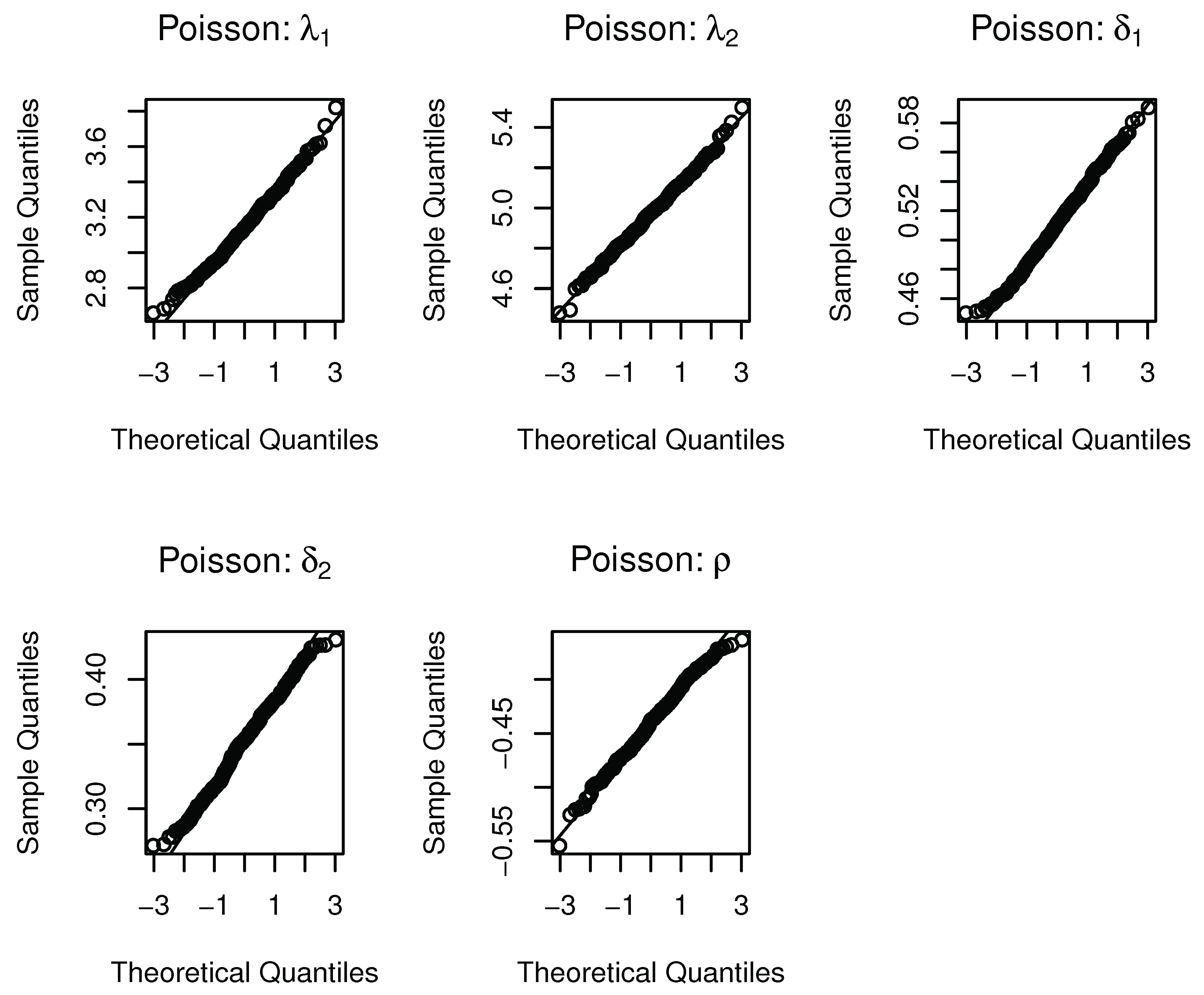
Table 2 and Table 3 demonstrate that the parameter estimates converge to the true values, with standard errors decreasing as the sample size increases. Further, we observe that both the MSE and MAE for the parameter estimates decrease as the sample size increases. This pattern is expected, since larger sample sizes provide more information about the underlying dependence structure, leading to more accurate and stable parameter estimates. In practical terms, as we increase the sample size, the parameter estimates produced by the MLE approach become more precise, resulting in smaller bias and reduced variability. Figure 1 and Figure 2 present the Q–Q plots for the parameter estimates obtained using Poisson marginals. The Q–Q plots show that the empirical distribution of the parameter estimates aligns closely with the ${45}^0$ reference line, indicating that the sampling distribution of the estimates is approximately normal. This supports the asymptotic normality of the maximum likelihood estimates and suggests stable inference as sample size increases.

With the introduction of one additional parameter the Negative Binomial(NB) distribution is able to account for over-dispersion when compared to the Poisson distribution. We have performed simulations choosing the Gaussian copula for univariate and joint distributions with NB marginals.

Table 4. Parameter estimates using Gaussian copula for univariate and joint distributions with Negative Binomial marginals.

Sample Size	Parameter	Estimate	SE	MSE	MAE
50	${\lambda }_1\left(4\right)$	4.050	0.724	0.525	0.578
	${\kappa }_1\left(1.5\right)$	1.554	0.603	0.367	0.428
	${\lambda }_2\left(6\right)$	6.057	0.852	0.728	0.669
	${\kappa }_2\left(2.5\right)$	2.469	0.759	0.576	0.591
	${\delta }_1\left(0.3\right)$	0.265	0.127	0.017	0.105
	${\delta }_2\left(0.3\right)$	0.268	0.121	0.016	0.097
	$\rho \left(0.5\right)$	0.505	0.111	0.012	0.085
100	${\lambda }_1\left(4\right)$	4.098	0.506	0.265	0.405
	${\kappa }_1\left(1.5\right)$	1.421	0.361	0.131	0.276
	${\lambda }_2\left(6\right)$	6.108	0.612	0.385	0.480
	${\kappa }_2\left(2.5\right)$	2.315	0.557	0.331	0.426
	${\delta }_1\left(0.3\right)$	0.278	0.087	0.008	0.071
	${\delta }_2\left(0.3\right)$	0.280	0.087	0.008	0.071
	$\rho \left(0.5\right)$	0.499	0.079	0.006	0.063
300	${\lambda }_1\left(4\right)$	4.085	0.291	0.092	0.241
	${\kappa }_1\left(1.5\right)$	1.451	0.173	0.044	0.175
	${\lambda }_2\left(6\right)$	6.118	0.375	0.155	0.311
	${\kappa }_2\left(2.5\right)$	2.342	0.292	0.133	0.308
	${\delta }_1\left(0.3\right)$	0.292	0.051	0.003	0.041
	${\delta }_2\left(0.3\right)$	0.286	0.049	0.003	0.041
	$\rho \left(0.5\right)$	0.496	0.045	0.002	0.036
1000	${\lambda }_1\left(4\right)$	4.101	0.175	0.041	0.162
	${\kappa }_1\left(1.5\right)$	1.362	0.093	0.027	0.145
	${\lambda }_2\left(6\right)$	6.088	0.192	0.044	0.164
	${\kappa }_2\left(2.5\right)$	2.253	0.148	0.083	0.252
	${\delta }_1\left(0.3\right)$	0.294	0.027	0.001	0.022
	${\delta }_2\left(0.3\right)$	0.292	0.029	0.001	0.024
	$\rho \left(0.5\right)$	0.497	0.024	0.001	0.019

and

Table 5. Parameter estimates using Gaussian copula for univariate and joint distributions with Negative Binomial marginals under negative cross-correlation.

Sample Size	Parameter	Estimate	SE	MSE	MAE
50	${\lambda }_1\left(4\right)$	4.052	0.731	0.535	0.589
	${\kappa }_1\left(1.5\right)$	1.593	0.564	0.326	0.417
	${\lambda }_2\left(6\right)$	6.109	0.915	0.848	0.716
	${\kappa }_2\left(2.5\right)$	2.586	0.712	0.514	0.535
	${\delta }_1\left(0.3\right)$	0.263	0.126	0.017	0.105
	${\delta }_2\left(0.3\right)$	0.260	0.125	0.017	0.105
	$\rho (-0.5)$	−0.490	0.112	0.012	0.087
100	${\lambda }_1\left(4\right)$	4.100	0.507	0.266	0.405
	${\kappa }_1\left(1.5\right)$	1.457	0.351	0.125	0.277
	${\lambda }_2\left(6\right)$	6.091	0.652	0.432	0.527
	${\kappa }_2\left(2.5\right)$	2.361	0.563	0.336	0.464
	${\delta }_1\left(0.3\right)$	0.278	0.089	0.008	0.073
	${\delta }_2\left(0.3\right)$	0.281	0.088	0.008	0.071
	$\rho (-0.5)$	−0.495	0.081	0.007	0.065
300	${\lambda }_1\left(4\right)$	4.095	0.299	0.098	0.248
	${\kappa }_1\left(1.5\right)$	1.372	0.174	0.046	0.181
	${\lambda }_2\left(6\right)$	6.128	0.361	0.146	0.301
	${\kappa }_2\left(2.5\right)$	2.259	0.288	0.140	0.316
	${\delta }_1\left(0.3\right)$	0.291	0.051	0.003	0.041
	${\delta }_2\left(0.3\right)$	0.289	0.052	0.003	0.042
	$\rho (-0.5)$	−0.497	0.047	0.002	0.037
1000	${\lambda }_1\left(4\right)$	4.108	0.201	0.052	0.181
	${\kappa }_1\left(1.5\right)$	1.419	0.136	0.025	0.131
	${\lambda }_2\left(6\right)$	6.092	0.218	0.056	0.189
	${\kappa }_2\left(2.5\right)$	2.402	0.236	0.065	0.024
	${\delta }_1\left(0.3\right)$	0.295	0.029	0.001	0.023
	${\delta }_2\left(0.3\right)$	0.289	0.032	0.001	0.027
	$\rho (-0.5)$	−0.487	0.027	0.001	0.024

demonstrate that the parameter estimates converge to the true values, with standard errors decreasing as the sample size increases. These results indicate that our proposed model is performing well with the Negative Binomial marginals for both negative and positive cross-correlations.

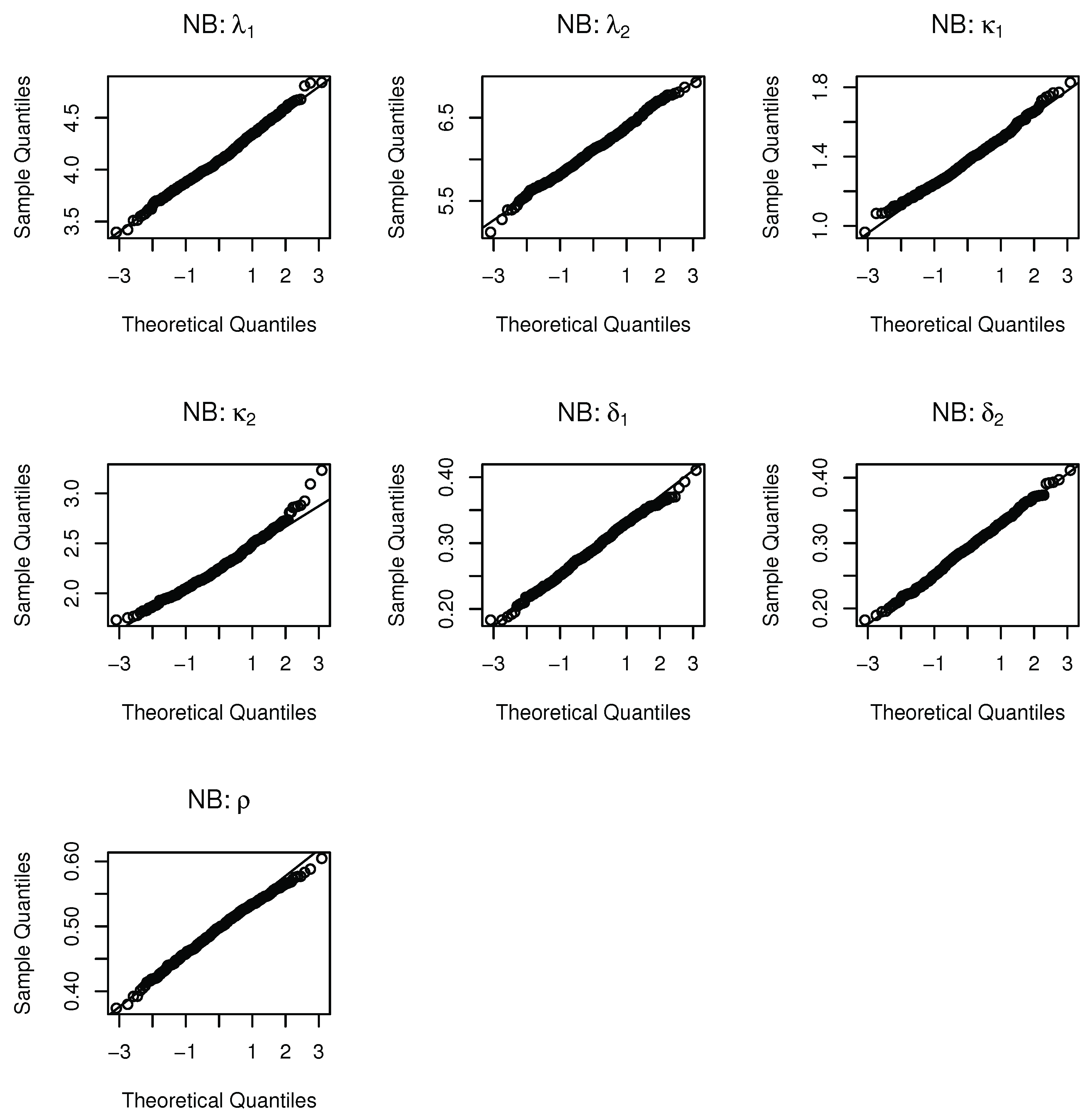
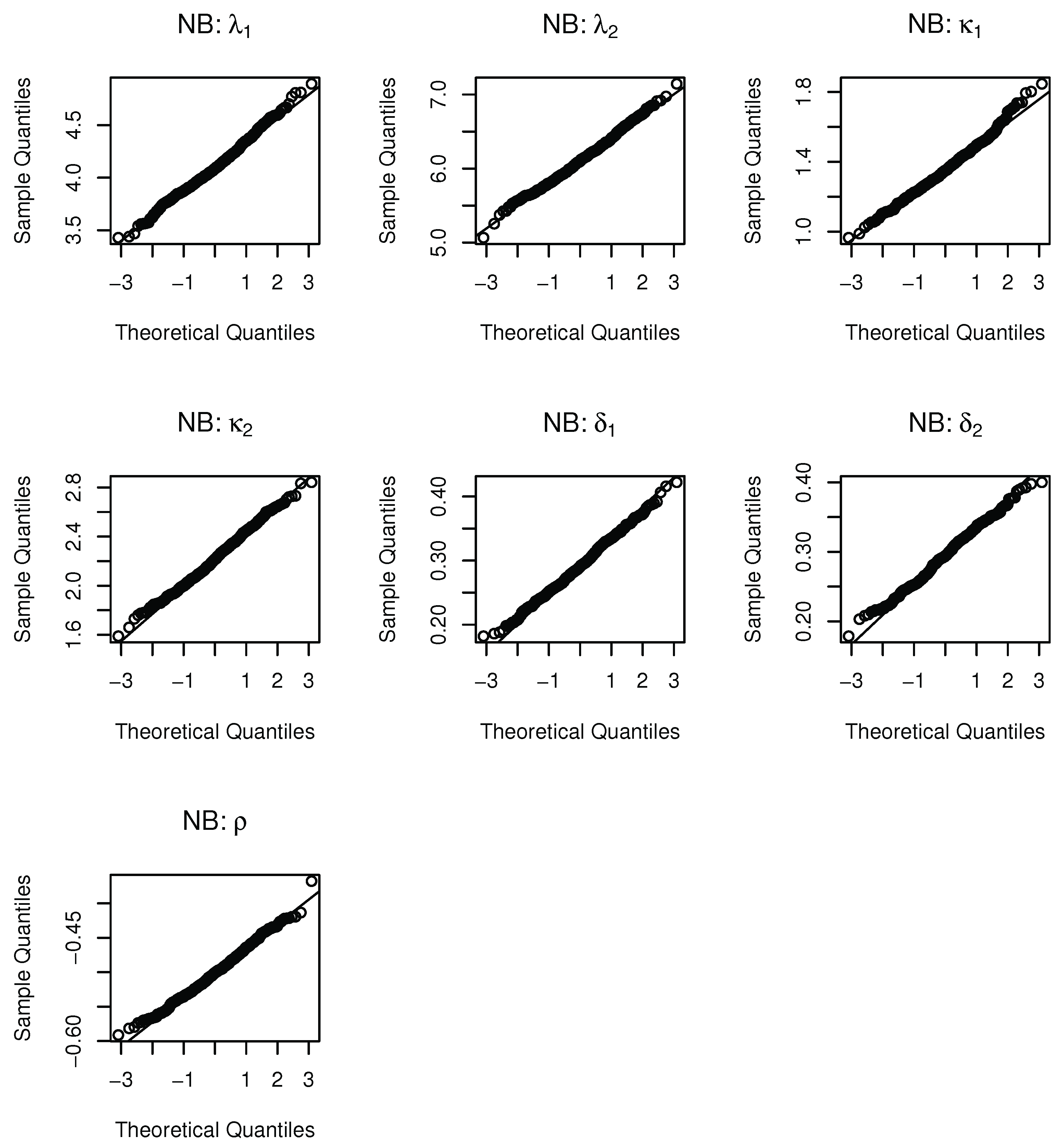
Figure 3 and Figure 4 present the Q–Q plots for the parameter estimates obtained using Negative Binomial marginals. The Q–Q plots show that the empirical distribution of the parameter estimates aligns closely with the ${45}^0$ reference line, indicating that the sampling distribution of the estimates is approximately normal.

3.2. Real-Data Application

In this application, we fit a copula-based bivariate model to analyze offense data from New South Wales, Australia. The dataset, obtained from the NSW Bureau of Crime Statistics and Research, is categorized by local government area, offense category, and month. The analyzed series consists of 228 paired monthly observations spanning from August 1995 to July 2014. This dataset has also been used in previous research (Yang et al. [18]). We selected sexual offense counts from Northern Beaches and Waverley city for analysis. The sexual offense counts are the sum of two subcategories:

• Sexual assault, and
• Sexual touching, sexual act and other sexual offenses.

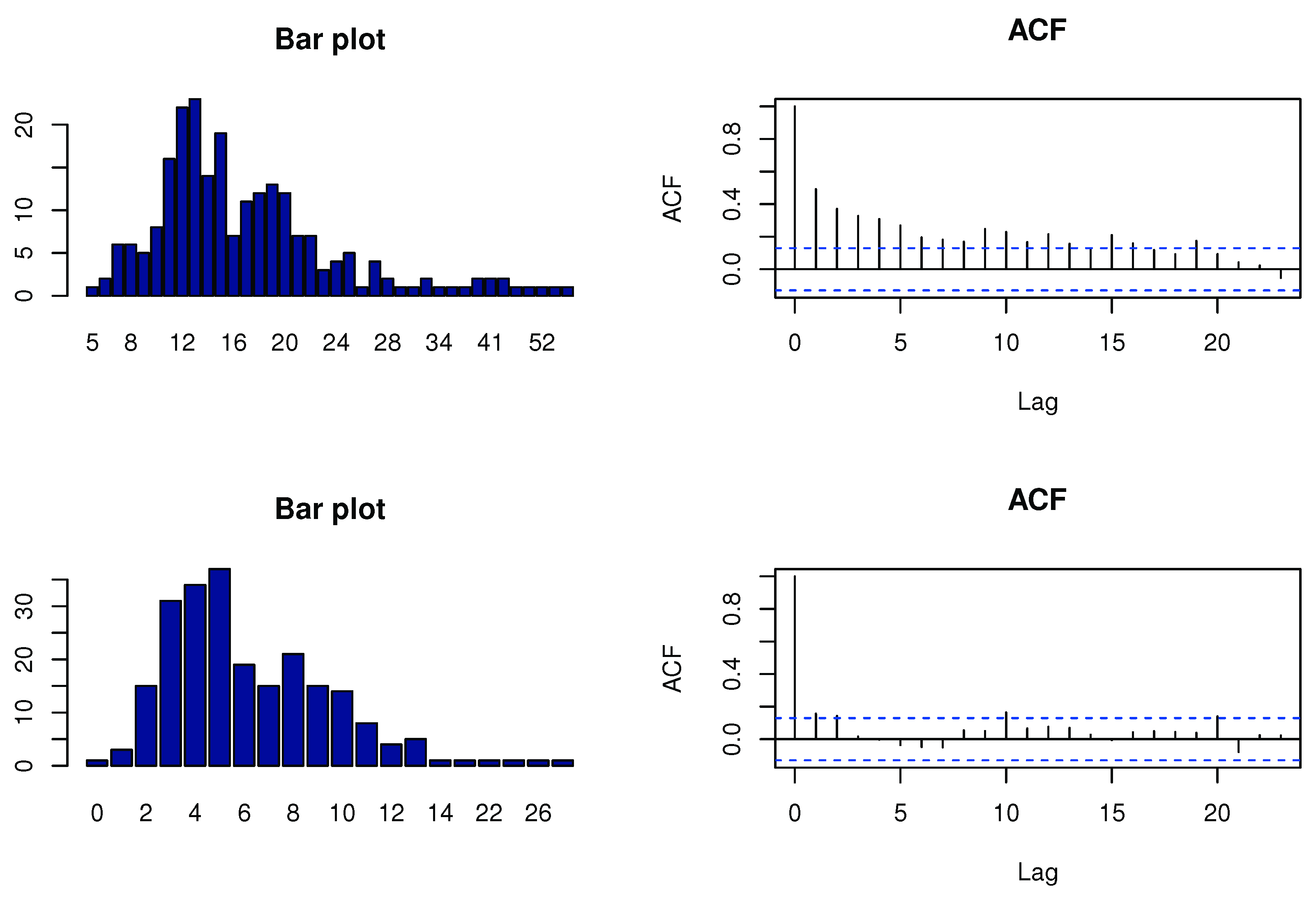
The empirical means for the two count time series are 17.452 (Northern Beaches) and 6.316 (Waverley), respectively. The monthly counts of sexual offenses for the two areas are shown in Figure 5. Compared to the Waverley count time series, the Northern Beaches count series exhibits higher counts and greater variation over time. Figure 6 presents bar plots of the count distributions and the sample autocorrelation functions (ACFs) for the two count series. The ACFs reveal clear serial dependence in both series. This observation motivates a detailed examination of serial and cross-series dependencies using the proposed copula-based bivariate model.

We do not observe any noticeable trends or seasonality in either count time series, supporting the stationarity assumption. Furthermore, the bar plots indicate that there is no evidence of zero-inflation in either series. We analyze these data using a copula-based bivariate model with Poisson and negative binomial marginals. The parameter estimates from our proposed model are compared with those from alternative bivariate count time series models, and model performance is evaluated using the AIC criterion. The manuscript by Yang et al. [18] shows the parameter estimates for BINAR (1) and all the other models presented in

Table 6. Parameter estimates of the sexual offense counts under different models.

Model	Parameter	Estimate	SE	AIC
BINAR(1)	${\alpha }_1$	0.276	0.018	3031.74
	${\alpha }_2$	0.099	0.028
	${\lambda }_1$	12.630	0.381
	${\lambda }_2$	5.676	0.199
	$\varphi$	0.405	0.235
BINDSETINAR(2,1)	${\alpha }_{1,1}$	0.000	0.041	2968.84
	${\alpha }_{1,2}$	0.285	0.023
	${\lambda }_1$	15.712	0.617
	${\alpha }_{2,1}$	0.004	0.068
	${\alpha }_{2,2}$	0.115	0.033
	${\lambda }_2$	5.973	0.344
$BTINA{R}_I\left(1\right)$	${\alpha }_{1,1}$	0.036	0.038	2955.53
	${\alpha }_{1,2}$	0.044	0.030
	${\alpha }_{2,1}$	0.317	0.021
	${\alpha }_{2,2}$	0.293	0.047
	${\lambda }_1$	15.329	0.596
	${\lambda }_2$	5.761	0.207
	$\varphi$	0.477	0.275
$BTINA{R}_{II}\left(1\right)$	${\alpha }_{1,1}$	0.200	0.020	3010.99
	${\alpha }_{1,2}$	0.019	0.098
	${\alpha }_{2,1}$	0.337	0.018
	${\alpha }_{2,2}$	0.094	0.040
	${\lambda }_1$	12.822	0.376
	${\lambda }_2$	5.862	0.393
	$\varphi$	0.389	0.245
$BTINA{R}_{III}\left(1\right)$	${\alpha }_{1,1}$	0.093	0.035	2960.57
	${\alpha }_{1,2}$	0.072	0.036
	${\alpha }_{2,1}$	0.331	0.021
	${\alpha }_{2,2}$	0.301	0.036
	${\lambda }_1$	14.544	0.565
	${\lambda }_2$	5.717	0.218
	$\varphi$	0.557	0.276

.

We compare our model with following bivariate integer-valued time series models using the AIC criterion.

• The Poisson BINAR(1) model (Pedeli and Karlis (2011) [19]).
• BINDSETINAR(2,1) model (Monteiro et al. (2012) [20]).
• The first order bivariate threshold integer-valued autoregressive process (BTINAR(1)) (Yang et al. [18]).

We have used several candidate copula families to model the joint distribution. Their corresponding AIC values are reported in

Table 7. AIC values of bivariate models fitted with different copula families.

	Marginal Distribution
Copula	Negative Binomial	Poisson
Gaussian	2719.38	3214.91
Frank	2747.75	3119.16
Clayton	2728.31	3168.33

to evaluate comparative model fit and identify the most suitable copula family. By comparing the observed AIC values, the models with Negative Binomial marginals outperformed those with Poisson marginals. Among these, the Gaussian copula with Negative Binomial marginals has the lowest AIC.

Table 8. Parameter estimates for the bivariate Poisson and Negative Binomial models.

Parameter	Poisson		Negative Binomial
	Estimate	SE	Estimate	SE
${\lambda }_1$	20.929	0.003	17.571	0.052
${\kappa }_1$			4.406	0.538
${\lambda }_2$	7.397	0.001	6.142	0.047
${\kappa }_2$			5.591	1.011
${\delta }_1$	0.341	0.025	0.377	0.129
${\delta }_2$	0.157	0.001	0.207	0.071
$\rho$	0.129	0.032	0.061	0.093
AIC	3214.91		2719.38

presents the parameter estimates for the copula-based model, where a Gaussian copula is used to construct the joint distribution with Poisson and Negative Binomial marginals. In this setting, parameters with subscript “1” correspond to the offense counts recorded in the Northern beaches, and parameters with subscript “2” correspond to the counts in Waverley city.

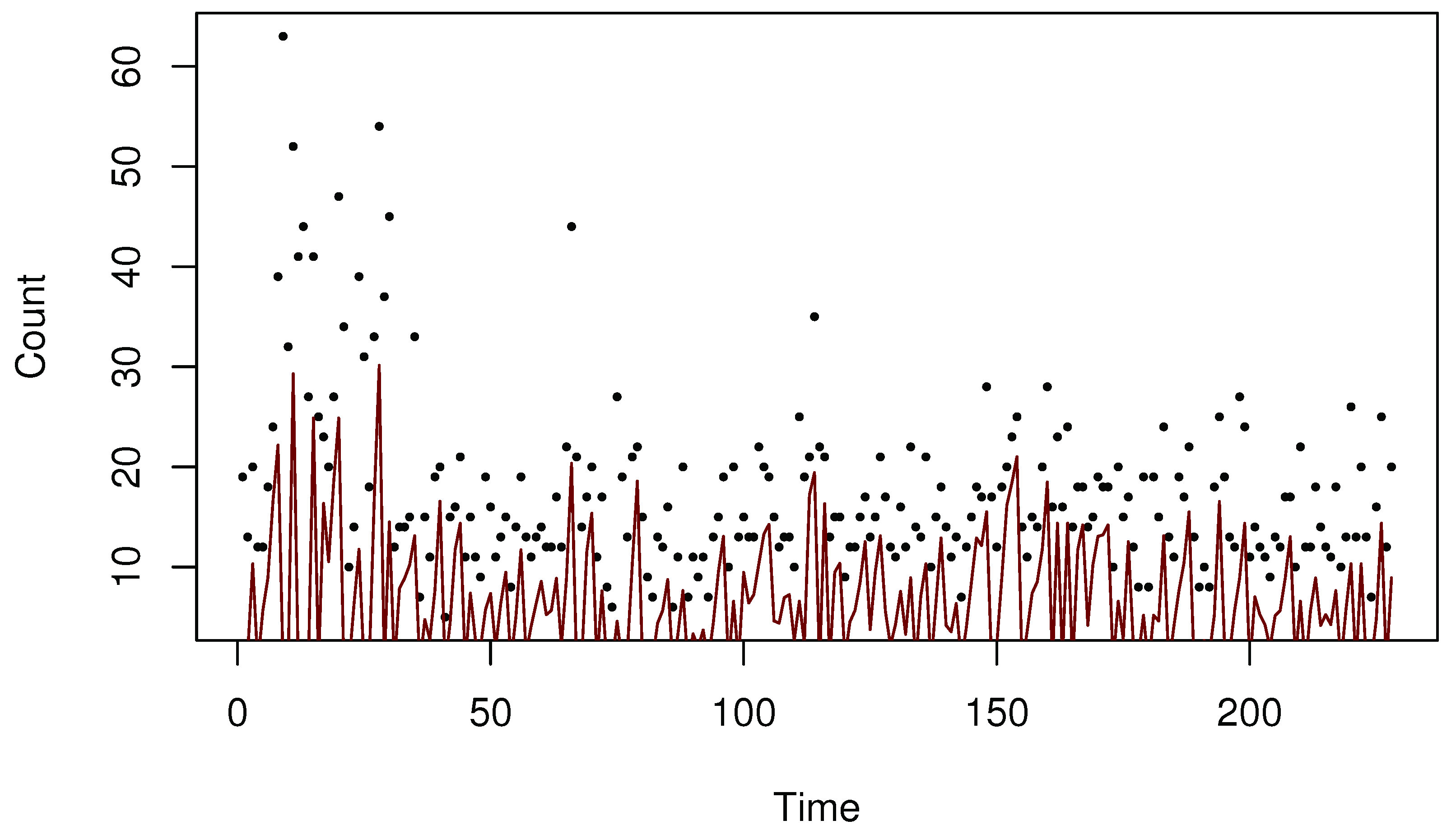
A comparison of the results shows that our proposed model with Negative Binomial marginals yields a lower AIC value (2719.38), indicating improved model fit. The parameter estimates for ${\lambda }_1$ and ${\lambda }_2$ exhibit smaller standard errors compared to those obtained from all other fitted models, which emphasizes the robustness of our proposed method. Since the model with Negative Binomial marginals can accommodate the over-dispersion present in the data, we can expect better performance compared to other fitted models.

Figure 7 and Figure 8 present the predicted values, which correspond to the conditional expectations of $Y_t$ given $Y_{t-1}$ under the bivariate negative binomial model for $t=2,\dots ,n$. Overall, the proposed model performs well, with some reduced accuracy for larger count values.

4. Discussion

In this paper, we introduced a class of bivariate integer-valued time series models based on copula theory. Serial dependence was captured through copula-based transition probabilities within a Markov chain framework, using both Poisson and Negative Binomial marginals. The cross-sectional dependence was modeled with a bivariate Gaussian copula. The performance of the likelihood-based estimation procedure was evaluated through simulation studies. Importance sampling was used to efficiently evaluate the bivariate normal integral. The models were also applied to a real-world count dataset using both marginal distributions. Model comparisons based on the AIC criterion indicated that the proposed approach with Negative Binomial marginals achieved the best fit. Both the simulation results and the empirical analysis confirmed the effectiveness of the proposed methodology.

As a future extension, we plan to construct a multivariate framework for higher-dimensional data using vine copulas.

References

1. Quoreshi, A.S. Bivariate time series modeling of financial count data. Commun. Stat.-Theory Methods 2006, 35, 1343–1358. [Google Scholar] [CrossRef]
2. Wang, K.; Lee, A.H.; Yau, K.K.; Carrivick, P.J. A bivariate zero-inflated Poisson regression model to analyze occupational injuries. Accid. Anal. Prev. 2003, 35, 625–629. [Google Scholar] [CrossRef] [PubMed]
3. Heinen, A.; Rengifo, E. Multivariate autoregressive modeling of time series count data using copulas. J. Empir. Financ. 2007, 14, 564–583. [Google Scholar] [CrossRef]
4. Karlis, D.; Pedeli, X. Flexible bivariate INAR (1) processes using copulas. Commun. Stat.-Theory Methods 2013, 42, 723–740. [Google Scholar] [CrossRef]
5. Ravishanker, N.; Venkatesan, R.; Hu, S. Dynamic models for time series of counts with a marketing application. In Handbook of Discrete-Valued Time Series; Chapman and Hall/CRC: Boca Raton, FL, USA, 2016. [Google Scholar]
6. Bradshaw, C.; Blei, D.M. A Bayesian model of underreporting for sexual assault on college campuses. Ann. Stat. 2024, 18, 3146–3164. [Google Scholar] [CrossRef]
7. Cui, Y.; Zhu, F. A new bivariate integer-valued GARCH model allowing for negative cross-correlation. Test 2018, 27, 428–452. [Google Scholar] [CrossRef]
8. Ahamad, N.; Gayah, V.V.; Donnell, E.T. Copula-based bivariate count data regression models for simultaneous estimation of crash counts based on severity and number of vehicles. J. Acc. Anal. Prev. 2023, 181, 106928. [Google Scholar] [CrossRef] [PubMed]
9. Jeng, A.H.; Singh, R.; Diawara, N.; Curtis, K.; Gonzalez, R.; Welch, N.; Jackson, C.; Jurgens, D.; Adikari, S. Application of wastewater-based surveillance and copula time-series model for COVID-19 forecast. Sci. Total Environ. 2023, 885, 163655. [Google Scholar] [CrossRef] [PubMed]
10. Xu, X.; Hardin, J.W. Regression models for bivariate count outcomes. Stata J. 2016, 16, 301–315. [Google Scholar] [CrossRef]
11. Alqawba, M.; Fernando, D.; Diawara, N. A class of copula-based bivariate poisson time series models with applications. Computation 2021, 9, 108. [Google Scholar] [CrossRef]
12. Nelsen, R.B. An Introduction to Copulas; Springer: Cham, Switzerland, 2007. [Google Scholar]
13. Joe, H. Dependence Modeling with Copulas; Chapman and Hall/CRC: Boca Raton, FL, USA, 2014. [Google Scholar]
14. Alqawba, M.; Diawara, N. Copula-based Markov zero-inflated count time series models with application. J. Appl. Stat. 2021, 48, 786–803. [Google Scholar] [CrossRef] [PubMed]
15. Panagiotelis, A.; Czado, C.; Joe, H. Pair copula constructions for multivariate discrete data. J. Am. Stat. Assoc. 2012, 107, 1063–1072. [Google Scholar] [CrossRef]
16. Genz, A.; Bretz, F. Computation of Multivariate Normal and t Probabilities; Springer Science & Business Media: Cham, Switzerland, 2009; Volume 195. [Google Scholar]
17. Hothorn, T.; Bretz, F.; Genz, A. On multivariate t and Gauss probabilities in R. Sigma 2001, 1000, 3. [Google Scholar]
18. Yang, K.; Zhao, Y.; Li, H.; Wang, D. On bivariate threshold Poisson integer-valued autoregressive processes. J. Metrika. 2023, 86, 931–963. [Google Scholar] [CrossRef]
19. Pedeli, X.; Karlis, D. A bivariate INAR (1) process with application. J. Stat. Model. 2011, 11, 325–349. [Google Scholar] [CrossRef]
20. Monteiro, M.; Scotto, M.G.; Pereira, I. Integer-valued self-exciting threshold autoregressive processes. Commun. Stat.-Theory 2012, 41, 2717–2737. [Google Scholar] [CrossRef]
Figure 1. Q–Q Plots of ML estimates for n = 1000 under positive cross-correlation with Poisson marginals.
Stats 08 00111 g001
Figure 2. Q–Q Plots of ML estimates for n = 1000 under negative cross-correlation with Poisson marginals.
Stats 08 00111 g002
Figure 3. Q–Q plots of the ML estimates for n = 1000 with positive cross-correlation with Negative Binomial marginals.
Stats 08 00111 g003
Figure 4. Q–Q plots of the ML estimates for n = 1000 with negative cross-correlation with Negative Binomial marginals.
Stats 08 00111 g004
Figure 5. Sexual offenses counts for Waverley and Northern beaches.
Stats 08 00111 g005
Figure 6. Bar plot and ACF for counts of offenses for Waverley (Top) and Northern beaches (Bottom).
Stats 08 00111 g006
Figure 7. Predicted values of the offense counts for the Waverley City based on the bivariate Negative Binomial model. Dots represent the observed counts, and the lines represent the predicted values.
Stats 08 00111 g007
Figure 8. Predicted values of the offense counts for the Northern Beaches based on the bivariate Negative Binomial model. Dots represent the observed counts, and the lines represent the predicted values.
Stats 08 00111 g008