Article

Analysis of the Truncated XLindley Distribution Using Bayesian Robustness

1
Probability Statistics Laboratory (LPS), Department of Mathematics, Badji Mokhtar University, BP12, Annaba 23000, Algeria
2
Department of Software and Information Systems Technologies, Faculty of New Information and Communication Technologies, University of Abdelhamid Mehri Constantine 2, Constantine 25000, Algeria
3
Laboratory of Statistics and Stochastic Processes, University of Djillali Liabes BP 89, Sidi Bel Abbes 22000, Algeria
*
Author to whom correspondence should be addressed.
Stats 2025, 8(4), 108; https://doi.org/10.3390/stats8040108
Submission received: 20 September 2025 / Revised: 31 October 2025 / Accepted: 2 November 2025 / Published: 5 November 2025
(This article belongs to the Special Issue Robust Statistics in Action II)

Abstract

In this work, we present a robust examination of the Bayesian estimators utilizing the two-parameter Upper truncated XLindley model, a unique Lindley model variant, and the oscillation of posterior risks. We provide the model in a censored scheme along with its likelihood function. The topic of sensitivity and robustness analysis of the Bayesian estimators was only covered by a small number of authors. As a result, very few apps have been created in this field. The oscillation of the posterior hazards of the Bayesian estimator is used to illustrate the method. By using a Monte Carlo simulation study, we show that, with the correct generalized loss function, a robust Bayesian estimator of the parameters corresponding to the smallest oscillation of the posterior risks may be obtained; robust estimators can be obtained when the parameter space is low-dimensional. The robustness and precision of Bayesian parameter estimation can be enhanced in regimes where the parameters of interest are of small magnitude.

1. Introduction

Statistical analysis is frequently heavily dependent on the assumed probability distributions; however, not all statistical problems follow the classical or standard probability distributions. In reliability and survival analysis, selecting an appropriate fundamental model is becoming increasingly important for new data analysis; even minor deviations from the fundamental model may have a major impact on the results.
New probability distributions have emerged as a crucial tool for enhancing statistical modeling in lifetime data modeling, survival research, and reliability analysis in recent years. Because of its adaptability in modeling data with non-monotonic hazard rates the Lindley and its generalized versions have drawn the most attention among them. Compared to traditional exponential or gamma models, the XLindley distribution in particular offers a better fit for a variety of lifespan data types. The examination of shortened versions of such distributions is practically significant because, in many real-world scenarios, the observed data are constrained or abbreviated because of experimental, financial, or physical constraints.
Newly founded distributions have been the subject of numerous studies lately, and truncated distributions have numerous uses; Bantan et al. [1] introduced the Truncated Inverted Kumaraswamy-generated family of distributions. Aldahlan et al. [2] introduced the truncated Cauchy power family of distributions. Mansour et al. [3] provided a new generalization of the reciprocal exponential model, Singh et al. [4] studied the modified Topp-Leone distribution with application to COVID-19 and reliability data. Elshahhat et al. [5] introduced the inverted hjorth distribution with applications in environmental and pharmaceutical Sciences.
The upper truncated XLindley distribution (UXLD), initially made clear by khoudja et al. [6], is inspired by a one-parameter distribution called XLindley distribution, which is a mixture of Exponential distribution and Lindley distribution. The XLindley distribution (XLD) is a straightforward and user-friendly tool for assessing a wide range of real-world data sets, including those pertaining to the corona, ebola, and nipah viruses. It provides satisfactory fits to a large number of data sets. For example, see the works of Ghitany et al. [7], Zeghoudi and Chouia [8], and Talhi and Aiachi [9].
The sensitivity of Bayesian analysis findings to the analysis’ inputs is an issue of robust Bayesian analysis. Rather than being explicitly described, a prior in robust Bayesian analysis is presumed to belong to a family of distributions, which results in a set of Bayes actions. Furthermore, although numerous studies have concentrated on estimating the XLindley parameters through classical approaches, scant attention has been directed toward its Bayesian analysis, particularly concerning model uncertainty and robustness issues.
Motivated by these observations, this paper aims to perform a comprehensive Bayesian robustness analysis of the truncated XLindley distribution, providing more reliable inference under prior misspecification and outlier contamination. The point estimation of the truncated XLindley distribution’s parameters is the main focus of the majority of current Bayesian approaches. In this work, we aim to perform a robust Bayesian analysis by examining the oscillations of the posterior risks associated with the parameter estimators. This gives us a numerical indicator of robustness by enabling us to evaluate how sensitive the Bayesian estimates are to changes in the prior or model assumptions. Our method offers a more robust framework for parameter inference under uncertainty by concentrating on the stability of the posterior risks, which goes beyond conventional estimation.
As per Mȩczarski and Zieliński’s [10] methodology, we suggest using an appropriate generalized loss function to do robustness and sensitivity analysis of the Bayesian estimators. The model’s genesis is presented in the Section 2. The Section 3 does a Bayesian robustness study of this model. In the Section 4, we used a generalized quadratic loss function. The study examines the Bayesian stability of the model’s two parameters. Analyzing the effectiveness of the Bayesian estimators is the focus of the Section 5, which involves an extensive simulation study.

2. Model’s Origins

Let ( X 1 , X 2 , …, X n ) be a random sample with density from UXLD ( α , β):
f U X L x , α , β = α 2 2 + α + x 1 + β 2 e α x + β x 1 + α 2 A β x ,
where x 0 ,     with   α > 0   and   β > 0 , where A β x = 1 + β 2 e β x 1 + β x .
The likelihood function that is derived from the observation x = {   x 1 , x 2 , …, x n } is
L x 1 , . . , , x n α , β = e i = 1 n α i + β x i α 2 n 1 + β 2 n 1 + α 2 n i = 1 n 2 + α + x i A β x i .
Assume that the prior of the parameters ( α , β) is π0 ( α , β). We obtain the associated posterior distribution by applying the Bayes rule:
π α ;   β x = L x ; α , β . π 0 α , β 0 + 0 + L x ; α , β . π 0 α , β d α   d β .
In most cases, the posterior density lacks a tractable formulation, in which case the Bayesian estimators can only be computed via Monte Carlo techniques. We will use the suggested approach to undertake a robust Bayesian analysis of this estimation in the following through Mȩczarski and Zieliński [10] methodology. The next section goes into detail about this procedure.

3. The Robustness of Bayesian Models

In statistical modeling and decision-making under uncertainty, Bayesian methods provide a coherent framework for updating beliefs in light of new evidence. However, Bayesian inferences often rely on assumptions about prior distributions, likelihood models, or hyperparameters, which may be imperfectly specified or only partially known. Bayesian robustness addresses the sensitivity of Bayesian conclusions to these assumptions, aiming to ensure that posterior inferences remain reliable even when the model is ambiguous or the prior is uncertain.
Robust Bayesian analysis investigates how variations in the prior, likelihood, or loss function influence posterior distributions, predictive outcomes, or decision-making criteria. Techniques such as prior sensitivity analysis, posterior predictive checks, and divergence measures (e.g., Kullback-Leibler divergence) are commonly used to quantify robustness. The goal is not only to detect potential vulnerabilities in Bayesian models but also to design models and priors that produce stable, trustworthy inferences under realistic conditions. Bayesian robustness is particularly relevant in high-stakes applications—such as medicine, finance, and engineering—where decisions based on fragile models can have significant consequences. By emphasizing resilience to model uncertainty, robust Bayesian methods bridge the gap between theoretical rigor and practical reliability, ensuring that probabilistic reasoning remains dependable in the face of ambiguity. For more details, one may refer to Chadli et al. [11], Berger et al. [12], and Micheas [13].

3.1. Basic Quadratic Loss Function

3.1.1. Stability for α in Bayesian Models

The prior densities of α and β are as follows when the following priors are taken into consideration for α and β, respectively: β ∼ non-informative and α ∼ Gamma ( a 0 , b 0 ), a 0 > 0, b 0 > 0.
π 0 α = b 0 a 0 α a 0 1 e α b 0 Γ a 0 ,
π 1 β = 1 β , β > 0 .
The Bayes theorem provides the joint posterior distribution of the parameters α and β as follows:
π α , β x = π 0 α π 1 β L x , α , β 0 + 0 + π 0 α π 1 β L x , α , β d α   d β .
This is typically stated more simply as
π α , β x π 0 α π 1 β L x , α , β .
Then,
π α , β x α e α b 0 + i = 1 n α x i + β x i α a 0 1 + 2 n 1 + α 2 n 1 + β 2 n β i = 1 n 2 + α + x i A β x i .
Nevertheless, the parameters α and β’s marginal posterior distributions do not match any known distributions. We employ Markov chain Monte Carlo (MCMC) techniques, particularly the Metropolis–Hastings algorithm within a Gibbs sampling (see, Gilks et al. [14]) in order to extract samples from the parameter’s marginal distributions.
The saved sample is α N = ( α 1 , …, α N ). The computation of the Bayesian estimator α ^ of α is performed with it. We find the mean under the quadratic loss function. Recall that a 0 and b 0 are prerequisites for our estimator. Thus, α ^ α 0 , b 0 = m e a n   α N is noted.
Assuming that the prior is not precisely specified, we use the Mȩczarski and Zieliński [10] methodology to perform the stability Bayesian analysis on α. Specifically, we retain the value b 0 fixed and take into account the parameter a 1 a a 2 rather than a 0 with a 1 and a 2 fixed. Next, we get the posterior risk PR (a) for α when a fluctuates between a 1 and a 2 .
P R a = E α α ^ a 0 , b 0 2 x = E α 2 x , a , b 0 + α ^ 2 a 0 , b 0 2 α ^ a 0 , b 0 E α x , a , b 0 .
where E α x , a , b 0 = 0 α π 0 α x , a , b 0 d α .
And the associated oscillation of the posterior risk, designated as R 1 , of the Bayesian estimator of α is
R 1 = max a 1 a a 2 P R a min a 1 a a 2 P R a .

3.1.2. Stability for β in Bayesian Models

We now employ a Gamma ( u 0 , v 0 ) prior for β and a non-informative prior for α . α and β have density priors that are, respectively,
π 0 α = 1 α   , α > 0 ,
π 1 β = v 0 u 0 β u 0 1 e β v 0 Γ u 0 .
Given the parameters α and β, the joint posterior distribution is given by
π α , β x = e β u 0 + i = 1 n α x i + β x i i = 1 n 2 + α + x i A β x i α 2 n 1 1 + α 2 n β t 0 1 1 + β 2 n .
Once again, we employ the Gibbs sampling with Metropolis–Hastings’s step to get the marginal distributions of the parameters.
Relying on Mȩczarski and Zieliński’s [10] methodology, we conduct a stability Bayesian analysis on β by holding constant the value v 0 and examining the parameter u 1 u u 2 , keeping u 1 and u 2 fixed. Next, we get the posterior risk PR(u) for β when u fluctuates between u 1 and u 2 .
P R u = E [ ( β β ^ ( u 0 , v 0 ) ) 2 x ] = E β 2 x ; u , v 0 + β ^ 2 u 0 , v 0 2 β ^ u 0 , v 0 E β x ; u , v 0 ,
where E β x ; u , v 0 = 0 α π 0 α x ; u , v 0 d β .
E β 2 x ; u , v 0 = 0 β 2 π 0 β x ; u , v 0 d β .
And the associated oscillation of the posterior risk, designated as R 2 , of the Bayesian estimate of β is
R 2 = max u 1 u u 2 P R u min u 1 u u 2 P R u .

3.2. Generalized Quadratic Loss Function

Now, we propose to apply the same concept as Larbi and Fellag [15] and consider a generalized quadratic loss function of the form L d ; t = t k ( d t ) 2 , where t is to be estimated, d is a Bayesian estimator, and k ∈ Z is the parameter of the generalized loss function. Notably, the basic quadratic loss function is derived for k = 0. Since the oscillation of the PR’s depends on k for both α and β, our goal is to determine if there exist values of k 0 such that the oscillation is smaller when we use the basic quadratic loss function (k = 0).

3.2.1. Bayesian Stability for α

The Bayesian estimation of α under the generalized loss function is
α ^ α 0 , b 0 , k = E α k + 1 x E α k x ;   k Ζ .
Next, the posterior risk for the α estimator is
P R a , k = E α k + 2 x ; a ,   b 0 2 α ^ a 0 , b 0 , k E α k + 1 x ; a ,   b 0 + E α k x ; a ,   b 0 α ^ a 0 , b 0 , k 2 .
Hence, the following formula provides the oscillation of the posterior risk of α.
R 1 = max a 1 a a 2 P R a min a 1 a a 2 P R a .

3.2.2. Bayesian Stability for β

For β, the Bayesian estimator is
β ^ u 0 , v 0 , k = E β k + 1 x E β k x ;   k Ζ .
The estimation of β’s posterior risk is provided by
P R β , k = E β k + 2 x ; u ,   v 0 2 β ^ u 0 , v 0 , k E β k + 1 x ; u ,   v 0 + E β k x ; u ,   v 0 β ^ u 0 , v 0 , k 2 .
And the posterior risk of β oscillates, which is
R 2 = max u 1 u u 2 P R u min u 1 u u 2 P R u .
Using MCMC techniques, the estimator, posterior risk, and oscillation formulas in the two scenarios must be numerically approximated.

4. Monte Carlo Study

4.1. Bayesian Stability for α

To check whether the stationary distribution of the Gibbs method is satisfactory, let us first provide an example.

Example

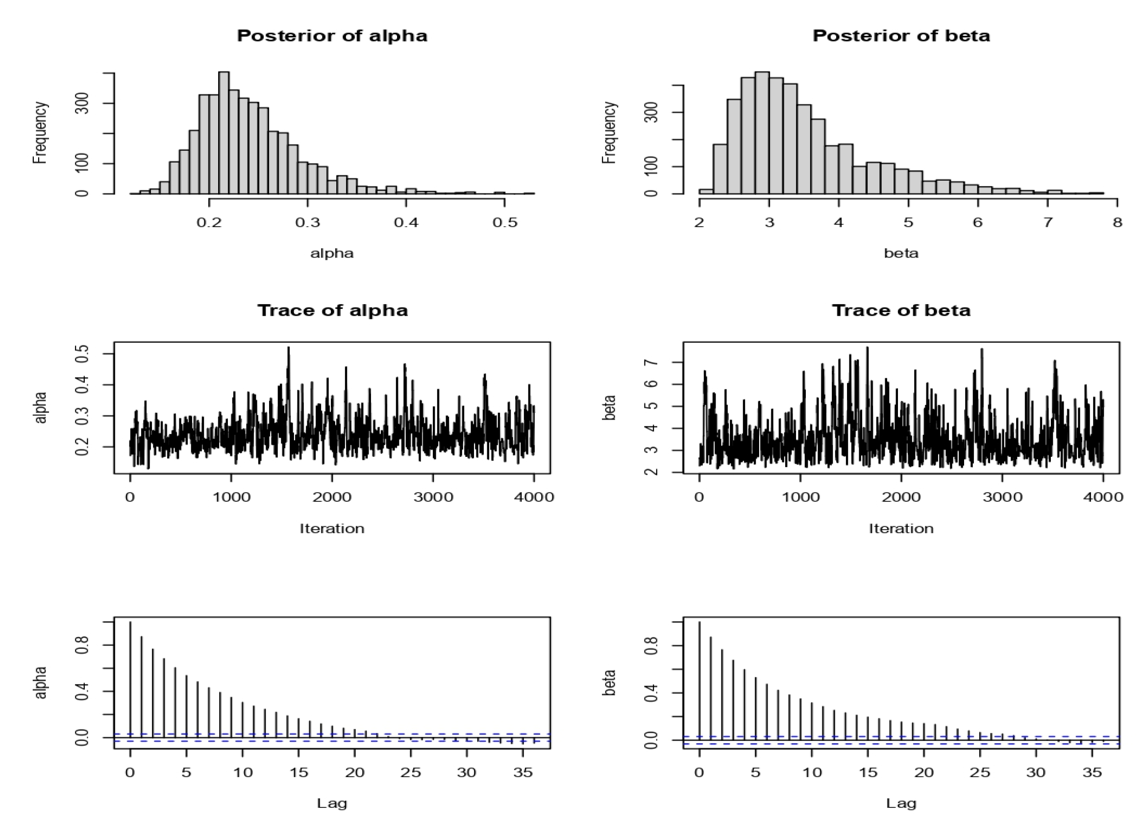
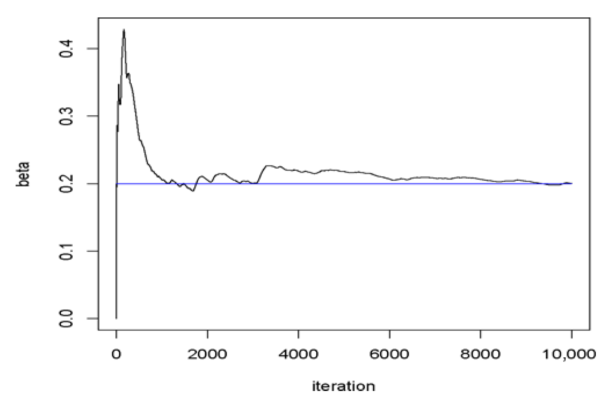
Let us consider a UXLD (0.5, 10) sample of size n = 50, where a 0 = 0.6 and b 0 = 8. We run 1000 iterations with B(1) = 50 as the starting value. The mean and values of α are shown in Figure 1. Furthermore, to ensure MCMC convergence, Figure 2 reported the histogram, trace, the auto-correlation function (ACF) plots of the two parameters, α and β.
Observe that α values fluctuate within a justifiable range surrounding the actual value. Furthermore, we note that the mean rapidly stabilizes at a value that is not far from the genuine value. Thus, it can be said that the stationary distribution has been roughly attained. Let us now examine three samples, n = 10, 30, and 50, where a 0 = 0.6 and b 0 = 8 are fixed. The posterior risks of the Bayesian estimators of α for various values of α and β are displayed in Table 1.
Let us now examine the stability of the α Bayesian estimators. To do this, we adjust a within the interval 0.5 < a ≤ 1.5 while maintaining b 0 = 8. The posterior risk oscillation is provided in Table 2.
Let us now examine the stability of the Bayesian estimators of α when k fluctuates under the generalized quadratic loss provided above. Since the outcomes remain constant with β, we can fix it to one without compromising generality. The simulation analysis is thus limited to α in {0.2, 0.4, 0.6, 1}. Additionally, we set b 0 = 8 and a 0 = 0.6 for each of the three samples with n = 10, 30, and 50.
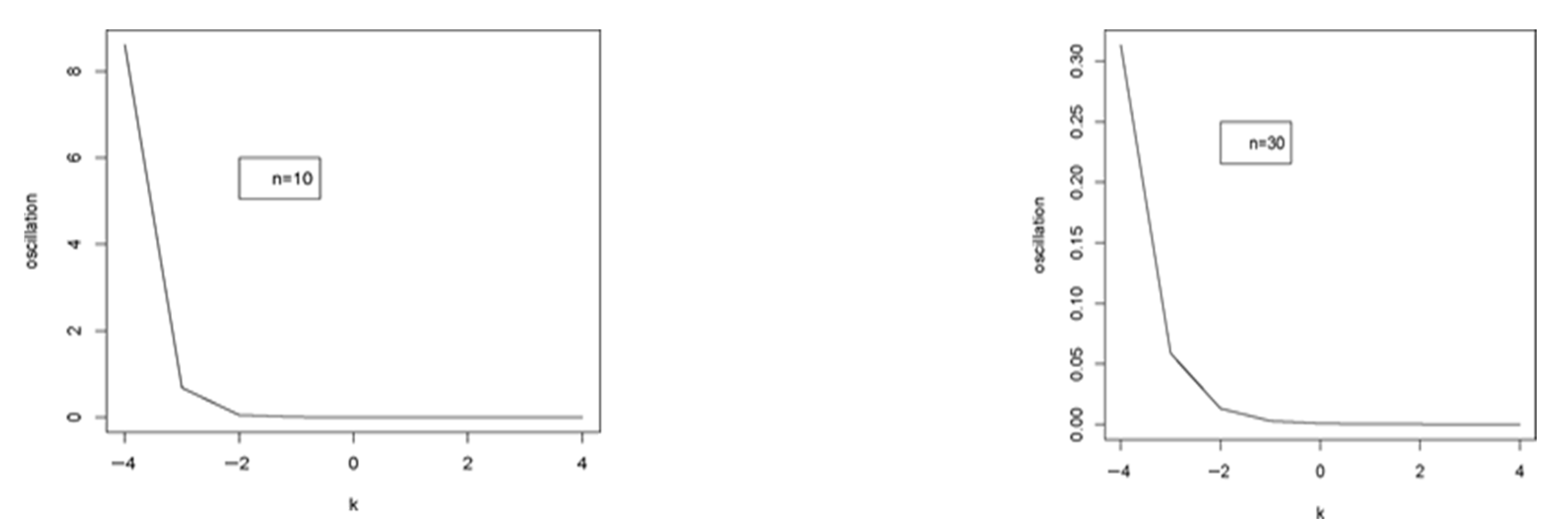
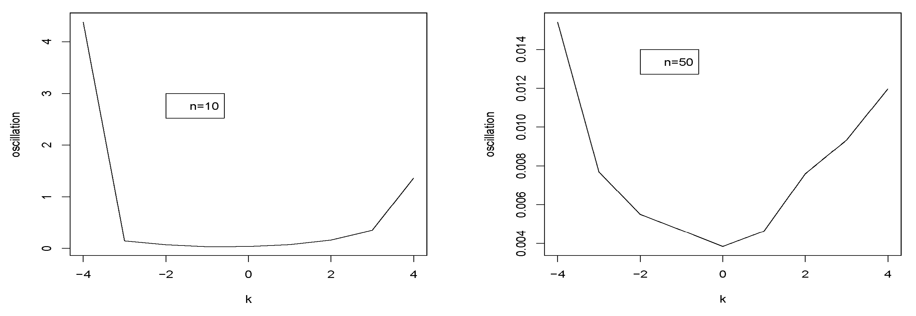
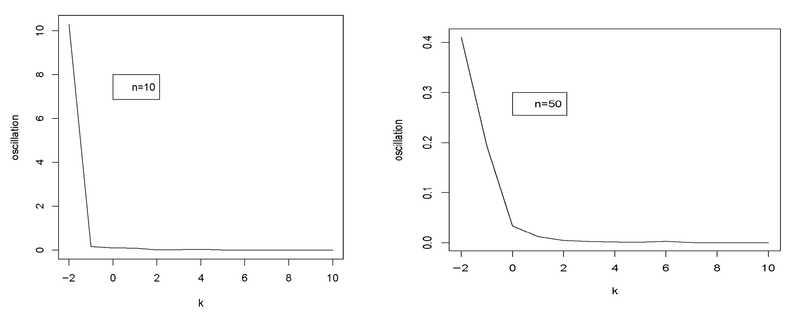
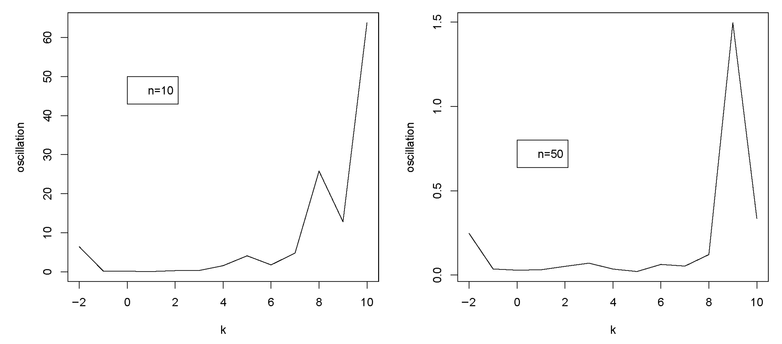
The posterior risk oscillations for various values of k are shown in Figure 2, Figure 3 and Figure 4. For large values of α , we observe that the values of the estimator of α are far from the genuine value (see Table 1). Additionally, it can be observed that, except in cases where α is high, the oscillation diminishes as n increases (see Table 2). It can be further stated that the oscillations are invariant with regard to β and less when α is near zero. We note that under the generalized quadratic loss function:
(i)
When k increases for n = 10, 30, 50, the oscillation diminishes for α = 0.2 (refer to Figure 3).
(ii)
The oscillation values for α = 0.4 fall to a specific value k0, after which they increase for n = 10, 30, and 50 (refer to Figure 4).
(iii)
When α = 1, the oscillation increases for k = 30, 50 and then reduces until a certain value k 1 at which point it grows (refer to Figure 5).
Subsequently, it may be inferred that across all examined values of α , we can enhance the robust α ’s Bayesian estimation. When α is small and k is sufficiently large, the optimal condition is achieved.

4.2. Bayesian Stability of β

As in the preceding subsection, let us first confirm whether the Gibbs algorithm’s stationary distribution is approximately achieved in this instance. Next, we take a look at the example that follows.

Example

Let us consider a UXLD (4, 0.3) sample of size n = 50, where u 0 = 0.3 and v 0 = 4. Since the conditional distribution β| α is unknown, we run 10,000 iterations with the initial value of B(1) = 0.1. Figure 6 displays the values of β that were acquired for each iteration along with its mean. Furthermore, to ensure MCMC convergence, Figure 7 reported the histogram, trace, and ACF plots of the two parameters, α and β.
It is evident that there is a reasonable range of variation in the values of β around the genuine value. Furthermore, we note that the mean rapidly stabilizes at a value that is not far from the genuine value. Thus, it can be said that the stationary distribution has been roughly attained. We examine three samples, n = 10, 30, and 50, with fixed u 0 = 0.3 and v 0 = 4. For certain values of α and β, we compute the posterior risks of the Bayesian estimators of β. Table 3 displays the acquired results.
Now, we adjust u in the interval 0.5 ≤ u ≤ 1.5 while maintaining v 0 = 4 constant in order to examine the stability of the Bayesian estimators of β. Table 4 provides the posterior risk oscillations.
Let us now examine the stability of the Bayesian estimators of β when k fluctuates under the generalized quadratic loss provided above. As the outcomes remain constant with α , we can fix α = 1 without sacrificing generality. The simulation investigation is then limited to β ∈ {0.08, 0.1, 0.4, 0.6, 0.8}. Additionally, we set v 0 = 4 and u 0 = 0.3 for each of the three samples with n = 10, 30, and 50.
The oscillations of the posterior risks for various values of k are shown in Figure 8 and Figure 9. For large values of β, we observe that the values of the estimator of β are far from the genuine value (see Table 3). Additionally, it can be observed that the oscillations are invariant with regard to α and less when β is near zero (see Table 4). We note that under the generalized quadratic loss function:
(i)
When k increases for n = 10, 50, the oscillation diminishes for small β (refer to Figure 8).
(ii)
As k increases for n = 10, 50, the oscillation values increase for β greater (see Figure 9).
Thus, when β has very small values, we can say that the robust Bayesian estimation of β can be improved.

5. Conclusions

This paper employs a particular methodology to perform robustness and sensitivity analysis of the Bayesian estimators of an upper truncated XLindley model. Two parameters were taken into consideration, and the robustness of the posterior risk was examined in terms of its oscillation. Then, we demonstrated that robust estimators may be derived for the parameters when they are not high under an appropriate generalized loss function using an exhaustive Monte Carlo technique.

Author Contributions

All authors contributed equally. All authors have read and agreed to the published version of the manuscript.

Funding

There are no funds received for this paper.

Data Availability Statement

The data used in this paper were generated through simulation as described in the Monte Carlo study section.

Conflicts of Interest

The authors declare no conflicts of interest.

References

  1. Bantan, R.A.R.; Jamal, F.; Chesneau, C.; Elgarhy, M. Truncated Inverted Kumaraswamy Generated Family of Distributions with Applications. Entropy 2019, 21, 1089. [Google Scholar] [CrossRef]
  2. Aldahlan, M.A.; Jamal, F.; Chesneau, C.; Elgarhy, M.; Elbatal, I. The Truncated Cauchy Power Family of Distributions with Inference and Applications. Entropy 2020, 22, 346. [Google Scholar] [CrossRef]
  3. Mansour, M.M.; Butt, N.S.; Yousof, H.; Ansari, S.I.; Ibrahim, M. A Generalization of Reciprocal Exponential Model: Clayton Copula, Statistical Properties and Modeling Skewed and Symmetric Real Data Sets: A Generalization of Reciprocal Exponential Model. Pak. J. Stat. Oper. Res. 2020, 16, 373–386. [Google Scholar] [CrossRef]
  4. Singh, B.; Tyagi, S.; Singh, R.P.; Tyagi, A. Modified Topp-Leone Distribution: Properties, Classical and Bayesian Estimation with Application to COVID-19 and Reliability Data. Thail. Stat. 2025, 23, 72–96. [Google Scholar]
  5. Elshahhat, A.; Abo-Kasem, O.E.; Mohammed, H.S. The Inverted Hjorth Distribution and Its Applications in Environmental and Pharmaceutical Sciences. Symmetry 2025, 17, 1327. [Google Scholar] [CrossRef]
  6. Khodja, N.; Aiachi, H.; Talhi, H.; Benatallah, I.N. The truncated XLindley distribution with classic and Bayesian inference under censored data. Adv. Math. Sci. J. 2021, 10, 1191–1207. [Google Scholar]
  7. Ghitany, M.E.; Al-Mutairi, D.K.; Nadarajah, S. Zero-truncated Poisson–Lindley distribution and its application. Math. Comput. Simul. 2008, 79, 279–287. [Google Scholar] [CrossRef]
  8. Zeghdoudi, H.; Chouia, S. The XLindley Distribution: Properties and Application. J. Stat. Theory Appl. 2021, 20, 318–327. [Google Scholar] [CrossRef]
  9. Talhi, H.; Aiachi, H. On Truncated Zeghdoudi Distribution: Posterior Analysis under Different Loss Functions for Type II Censored Data. Pak. J. Stat. Oper. Res. 2021, 17, 497–508. [Google Scholar] [CrossRef]
  10. Mȩczarski, M.; Zieliński, R. Stability of the Bayesian estimator of the Poisson mean under the inexactly specified gamma prior. Statist. Probab. Lett. 1991, 12, 329–333. [Google Scholar] [CrossRef]
  11. Chadli, A.; Talhi, H.; Fellag, H. Comparison of the Maximum Likelihood and Bayes Estimators of the parameters and mean Time Between Failure for bivariate exponential Distribution under different loss functions. Afr. Stat. 2013, 8, 499–514. [Google Scholar]
  12. Berger, J.O.; Rios Insua, D.; Ruggeri, F. Bayesian robustness. In Robust Bayesian Analysis; Insua, D.R., Ruggeri, F., Eds.; Springer: New York, NY, USA, 2000. [Google Scholar]
  13. Micheas, A.C. A Unified Approach to Prior and Loss Robustness. Comm. Statist. Theory Methods 2006, 35, 309–323. [Google Scholar] [CrossRef]
  14. Gilks, W.R.; Richardson, S.; Spiegelhalter, D.J. Introducing Markov Chain Monte Carlo. In Markov Chain Monte Carlo in Practice; CRC Press: Boca Raton, FL, USA, 1995; pp. 1–17. [Google Scholar]
  15. Larbi, L.; Fellag, H. Robust bayesian analysis of an autoregressive model with exponential innovations. Afr. Stat. 2016, 11, 955–964. [Google Scholar] [CrossRef]
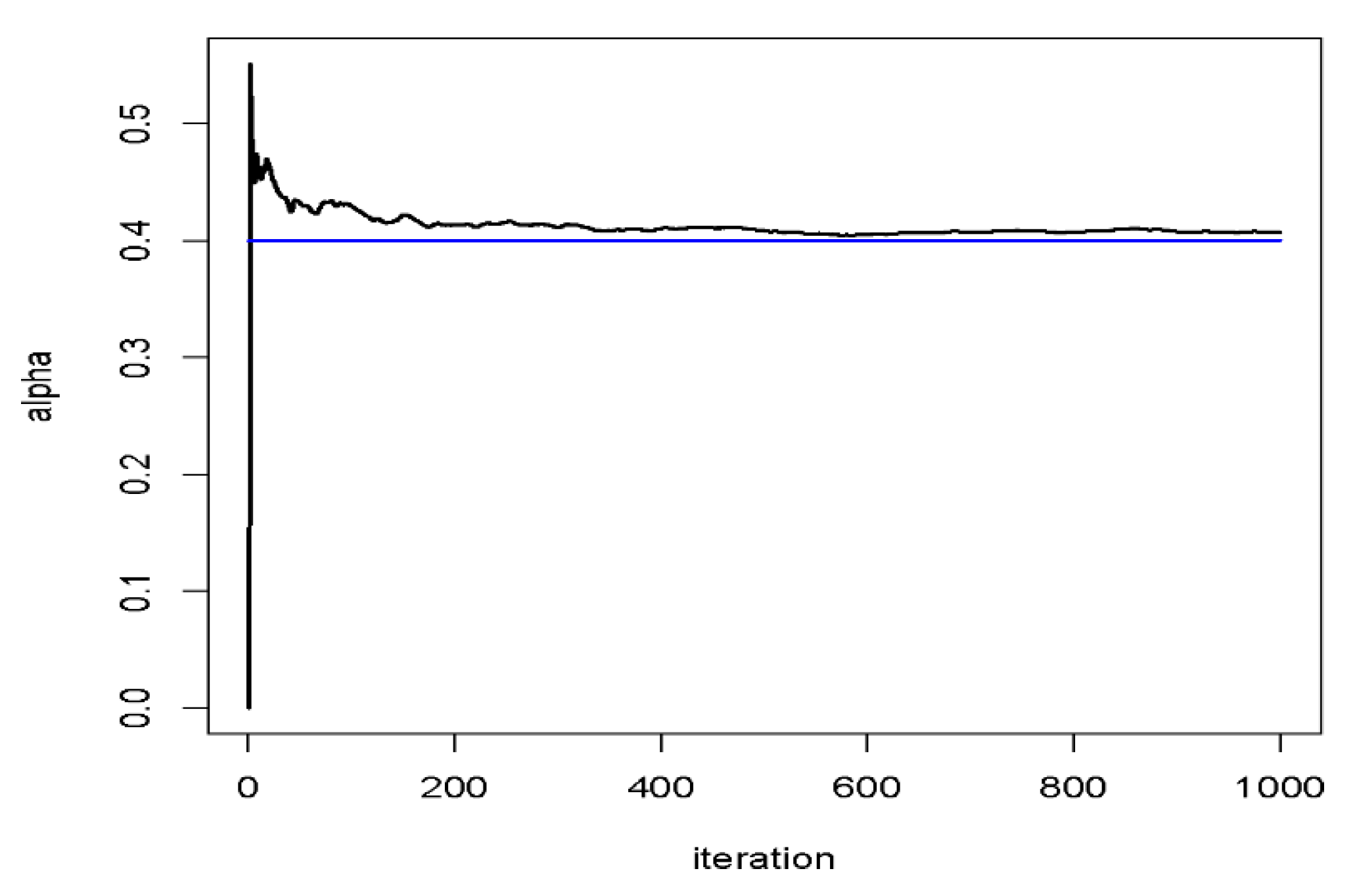
Figure 1. Changes in the values of α using the mean.
Stats 08 00108 g001
Figure 2. MCMC convergence plot of the UXLD (Stability for α ).
Stats 08 00108 g002
Figure 3. Changes in the PR oscillation with k for α when n = 10, 30, α = 0.2.
Stats 08 00108 g003
Figure 4. Changes in the PR oscillation with k for α when n = 10, 50, α = 0.4.
Stats 08 00108 g004
Figure 5. Changes in the PR oscillation with k for α when n = 10, 30 and α = 1.
Stats 08 00108 g005
Figure 6. Variation between β values and its mean.
Stats 08 00108 g006
Figure 7. MCMC convergence plot of the UXLD (Stability of β).
Stats 08 00108 g007
Figure 8. Changes in the PR oscillation with k for β when n = 10, 50, β = 0.08.
Stats 08 00108 g008
Figure 9. Changes in the PR oscillation with k for β when n = 10 and 50 and β = 0.4.
Stats 08 00108 g009
Table 1. α estimators for n = 10, 30, 50, with PRs in brackets, for a 0 = 0.6 and b 0 = 8.
α βn
103050
0.20.1646 (0.0025)0.2312 (0.0028)0.2234 (0.0015)
0.210.1867 (0.0041)0.2002 (0.0017)0.21208 (0.0012)
50.1423 (0.0020)0.2062 (0.0018)0.2869 (0.0025)
200.3213 (0.0113)0.1853 (0.0017)0.2052 (0.0012)
0.20.3340 (0.0265)0.3032 (0.0044)0.3264 (0.0035)
0.410.3327 (0.0139)0.5600 (0.0190)0.4596 (0.0074)
50.3505 (0.0146)0.4344 (0.0115)0.4715 (0.0089)
200.3876 (0.0189)0.2611 (0.0034)0.4063 (0.0056)
0.20.4692 (0.0325)0.5974 (0.0303)0.6318 (0.0182)
110.4955 (0.0317)0.7672 (0.0466)0.7225 (0.0264)
50.4199 (0.0249)0.5528 (0.0198)0.6288 (0.0165)
200.43611 (0.0463)0.5718 (0.0217)0.5940 (0.0146)
0.21.1850 (0.1388)3.4193 (0.3725)5.6590 (0.6387)
2011.2088 (0.1401)0.9099 (0.1030)1.2388 (0.1325)
50.8152 (0.0879)0.8236 (0.1358)1.2353 (0.3469)
200.7521 (0.0571)0. 9499 (0.0787)1.7520 (0.1229)
Table 2. PR oscillations of α estimators for n = 10, 30, and 50 when a 0 = 0.6 and b 0 = 8.
α βn
103050
0.20.20.00090.00150.0009
10.00190.00140.0002
50.00180.00040.0004
200.00510.00050.00007
0.20.02770.00060.0005
0.410.00890.00880.0010
50.04520.00810.0034
200.01460.00080.0007
0.20.00790.00580.0031
110.01400.00700.0040
50.00230.00260.0024
200.01670.00260.0019
0.20.03330.08640.1383
2010.03750.36690.3928
50.17540.40660.3588
200.05990.21780.5529
Table 3. β estimators for n = 10, 30, 50, with PR’s enclosed in brackets, for u 0 = 0.3 and v 0 = 4.
α βn
103050
0.20.20.1696 (0.0212)0.1096 (0.0050)0.1825 (0.0251)
10.0831 (0.0089)0.2009 (0.0150)0.1129 (0.0020)
50.16022 (0.0197)0.1500 (0.0273)0.1920 (0.0286)
100.1805 (0.0264)0.2128 (0.0319)0.2615 (0.0965)
0.20.1530 (0.0207)0.1958 (0.0223)0.2729 (0.0207)
0.410.2817 (0.0382)0.2730 (0.0212)0.2864 (0.0202)
50.2004 (0.0222)0.2813 (0.0337)0.3828 (0.0474)
100.2120 (0.0316)0.2288 (0.0327)0.2710 (0.0230)
0.20.2919 (0.0489)0.3670 (0.0748)0.6435 (0.0671)
110.2221 (0.0334)0.4716 (0.0506)0.5565 (0.0565)
50.1857 (0.0354)0.4122 (0.0344)0.6075 (0.0589)
100.2620 (0.0417)0.2775 (0.0296)0.4035 (0.0471)
0.20.3519 (0.0929)0.6078 (0.0838)1.0438 (0.1725)
2010.4933 (0.0745)1.3863 (0.0312)1.8561 (0.4235)
50.3925 (0.0934)1.0965 (0.2054)1.5682 (0.2850)
100.4321 (0.0429)0.7656 (0.1948)1.3402 (0.2297)
Table 4. PR’s of β estimators oscillating for n = 10, 30, 50, and v 0 = 4 with u 0 = 0.3.
α βn
103050
0.20.20.07830.00490.0321
10.02530.02540.0213
50.25930.42730.3667
100.16690.25450.1618
0.20.04690.03700.0154
0.410.05750.02010.0155
50.05830.06060.1287
100.06520.11710.1121
0.20.06250.06830.0340
110.06280.03650.0306
50.08540.05470.0842
100.06540.06630.0725
0.20.30240.43660.3037
2010.24160.80710.8361
50.49730.27000.2904
100.38190.38200.2793
Disclaimer/Publisher’s Note: The statements, opinions and data contained in all publications are solely those of the individual author(s) and contributor(s) and not of MDPI and/or the editor(s). MDPI and/or the editor(s) disclaim responsibility for any injury to people or property resulting from any ideas, methods, instructions or products referred to in the content.