Abstract
This study presents a comprehensive framework for agro-meteorological prediction, combining stochastic modeling, machine learning techniques, and environmental feature engineering to address challenges in yield prediction and wind behavior modeling. Focused on mango cultivation in the Mediterranean region, the workflow integrates diverse datasets, including satellite-derived variables such as NDVI, soil moisture, and land surface temperature (LST), along with meteorological features like wind speed and direction. Stochastic modeling was employed to capture environmental variability, while a proxy yield was defined using key environmental factors in the absence of direct field yield measurements. Machine learning models, including random forest and multi-layer perceptron (MLP), were hybridized to improve the prediction accuracy for both proxy yield and wind components (U and V that represent the east–west and north–south wind movement). The hybrid model achieved mean squared error (MSE) values of 0.333 for U and 0.181 for V, with corresponding R2 values of 0.8939 and 0.9339, respectively, outperforming the individual models and demonstrating reliable generalization in the 2022 test set. Additionally, although NDVI is traditionally important in crop monitoring, its low temporal variability across the observation period resulted in minimal contribution to the final prediction, as confirmed by feature importance analysis. Furthermore, the analysis revealed the significant influence of environmental factors such as LST, precipitable water, and soil moisture on yield dynamics, while wind visualization over digital elevation models (DEMs) highlighted the impact of terrain features on the wind patterns. The results demonstrate the effectiveness of combining stochastic and machine learning approaches in agricultural modeling, offering valuable insights for crop management and climate adaptation strategies.
1. Introduction
Agro-meteorological prediction is pivotal in modern agriculture, offering insights that enhance crop productivity and mitigate climate-related risks. By integrating satellite observations, meteorological data, and computational models, researchers can better understand the complex interactions between environmental factors and crop performance [1]. This study presents a comprehensive workflow for agro-meteorological prediction, focusing on mango cultivation in the Mediterranean region. The methodology combines stochastic modeling and machine learning techniques to address the challenges of data scarcity and environmental variability.
Agricultural systems are inherently complex, with nonlinear interactions among variables such as temperature, soil moisture, solar radiation, and wind dynamics. Traditional deterministic models often fall short in capturing this complexity, leading to less accurate predictions. Stochastic modeling has emerged as a powerful tool to address these limitations, effectively incorporating random fluctuations and uncertainties inherent in agricultural systems. For instance, a study on farmland irrigation scheduling utilized a multistage stochastic programming model to maximize annual profit under uncertain conditions, including crop prices and water availability [2].
A significant challenge in agro-meteorological modeling is the lack of direct yield data, especially in remote or large-scale agricultural systems. To overcome this, researchers often define a proxy yield that combines key environmental indicators such as vegetation health (NDVI) and water availability (soil moisture) [1,3]. This approach allows for the estimation of crop yields in the absence of direct measurements. For example, integrating remote sensing data with crop models has been shown to improve yield estimation accuracy, providing a viable alternative when field data are unavailable [4].
The integration of stochastic modeling and machine learning offers a robust framework for agro-meteorological prediction. Stochastic models account for random environmental fluctuations in natural systems such as marine ecosystems [5,6,7,8], while machine learning algorithms, such as random forests, capture complex, nonlinear relationships among variables. This combined approach has been applied in various agricultural contexts. For instance, a study on agricultural irrigation water allocation developed a two-stage chance-constrained programming model to optimize water use under uncertainty, demonstrating the effectiveness of combining stochastic optimization with data-driven methods [7,8].
Mango (Mangifera indica) is a high-value tropical fruit with increasing global production. According to FAO statistics (2023), mango production exceeded 57 million tons globally, and due to climate warming and favorable microclimates, mango cultivation is expanding in Southern Europe, particularly in Mediterranean regions such as Italy and Spain [9]. Recent studies have highlighted the sensitivity of mango production to environmental variables such as LST, solar radiation, and soil moisture, necessitating accurate and region-specific yield forecasting systems [10,11].
The machine learning models employed in this study include random forest (RF), multi-layer perceptron (MLP), and gradient boosting (GB), which are extensively utilized in meteorological forecasting tasks such as rainfall, evapotranspiration, and wind speed prediction. For instance, RF has been effectively applied to predict agricultural droughts, outperforming other models in forecasting the Standardized Precipitation Evapotranspiration Index (SPEI) in Central Europe [12]. MLPs have demonstrated superior performance in total cloud cover prediction, capturing complex nonlinear relationships in atmospheric data [13]. GB techniques, particularly extreme gradient boosting (XGBoost), have shown high accuracy in merging satellite and ground-based precipitation data, enhancing the reliability of precipitation datasets [14]. These models are adept at capturing the nonlinearities and multivariate dependencies inherent in agro-environmental data, thereby improving predictive performance in complex agricultural systems.
In recent years, climate change has significantly impacted agricultural practices in the Mediterranean region, leading to the introduction of tropical and subtropical crops such as mangoes. Rising temperatures and altered precipitation patterns have created favorable conditions for mango cultivation in areas like Sicily, Italy. Farmers have transitioned from traditional crops to mangoes, capitalizing on the higher market value and increasing consumer demand [15,16]. This shift not only diversifies agricultural production but also presents new challenges in crop management and yield prediction, necessitating advanced agro-meteorological models.
Wind behavior significantly influences agricultural systems, affecting crop growth, pollination, and physical stress on plants. Understanding wind dynamics is essential for developing protective measures and optimizing crop yield predictions. Wind-induced plant movement can alter growth rates and leaf morphology, while high winds may cause physical damage such as leaf tearing and abrasion [17].
Accurate modeling of wind components, specifically the zonal (U) and meridional (V) components, is crucial for understanding regional wind behavior in agricultural landscapes. Traditional numerical weather prediction models often lack the spatial resolution required for precise agricultural applications [18]. To address this, high-resolution wind speed forecast systems have been developed, coupling numerical weather prediction with machine learning techniques to provide detailed wind information beneficial for agricultural management [18,19].
Machine learning models, such as random forests and multi-layer perceptrons, have been employed to predict wind components effectively. These models can capture complex, nonlinear relationships between environmental variables and wind behavior, enhancing the accuracy of wind predictions. Combining multiple models through ensemble methods further improves predictive performance by leveraging the strengths of each approach [19].
Understanding wind behavior is also crucial for mitigating its mechanical effects on crops. Wind can cause direct mechanical damage, including leaf tearing and abrasion, which adversely affect crop yields. Implementing windbreaks and other protective measures can help reduce these negative impacts, underscoring the importance of an accurate modeling of the wind behavior in agricultural planning [20].
The main hypotheses of this study are as follows: (1) proxy yield can be effectively estimated using a combination of satellite-based environmental indicators and machine learning models, and (2) a hybrid model integrating multiple ML methods will outperform single-model baselines for both yield and wind prediction. The specific objectives are the following: (i) to define a proxy yield model incorporating stochastic components, (ii) to evaluate RF, MLP, and GB models against this target, (iii) to build a hybrid U/V wind model and analyze its residual performance, and (iv) to perform sensitivity, noise robustness, and regression-based relevance analysis to validate the stability and interpretability of results.
Mango cultivation is particularly sensitive to environmental changes, including temperature extremes, wind patterns, and soil moisture variability. By applying a combined stochastic and machine learning approach, this study aims to develop a predictive framework capable of providing accurate yield estimates for mango farms in the Mediterranean region. This methodology not only addresses the challenges of data scarcity but also offers a scalable solution adaptable to various crops and regions.
2. Material and Methods
Effective agro-meteorological prediction relies on the integration of diverse datasets capturing environmental, geospatial, and meteorological variables.
2.1. Data Sources and Types
2.1.1. Satellite Data
- MODIS (MOD13A1): Provides the Normalized Difference Vegetation Index (NDVI), a proxy for vegetation health. The data have a 500 m spatial resolution and a 16-day temporal frequency, making it suitable for tracking crop growth patterns over time [21].
- SMAP (Soil Moisture Active Passive): Offers soil moisture measurements at a 9 km resolution, critical for understanding water availability for crops under varying climatic conditions [22].
- Digital Elevation Model (DEM): Terrain data, including slope and aspect, were derived from the Shuttle Radar Topography Mission (SRTM). This dataset provides 30 m spatial resolution, allowing for detailed terrain analysis [23].
- Land Surface Temperature (LST): Retrieved from MODIS, these variables capture thermal conditions that influence crop growth and stress response [24].
2.1.2. Meteorological Data
Daily climate variables such as air temperature, wind speed, wind direction, relative humidity, surface pressure, and precipitation rates were sourced from global meteorological agencies like the National Oceanic and Atmospheric Administration (NOAA) and the European Centre for Medium-Range Weather Forecasts (ECMWF). These variables provide a detailed temporal resolution to monitor day-to-day variations in crop-relevant conditions [25,26].
2.1.3. Derived Features
- Kinetic Energy (KE): Quantifies the physical impact of wind on plants.
- Turbulence: Measures abrupt changes in wind speed, which may affect crop structure.
- Fourier Series Encodings: Captures seasonal trends in the data for both daily and annual cycles.
2.1.4. Challenges in Data Collection
The process of data collection faced several challenges:
Temporal and Spatial Harmonization: Satellite datasets (e.g., MODIS NDVI and SMAP soil moisture) are available at different temporal frequencies and resolutions. Meteorological data, updated daily, required synchronization with the coarser temporal resolution of satellite datasets.
Cloud Contamination: NDVI values are often affected by cloud cover in optical satellite imagery. This was mitigated using spatiotemporal interpolation techniques, which ensured continuity in vegetation health monitoring (see Section 2.2.5, Handling Missing Data).
Validation in Satellite Data: Satellite-derived measurements were cross-validated with limited ground-based observations to ensure their reliability for predictive modeling
2.2. Satellite Data Preparation
To ensure the data were consistent and suitable for modeling, the following preprocessing steps were performed:
2.2.1. Translating Satellite Imagery
Satellite data are typically delivered in a specific coordinate projection system. In this study, data were retrieved in the MODIS Sinusoidal Projection format and transformed into the WGS84 geographic coordinate system (latitude and longitude).
The MODIS Sinusoidal Projection coordinates were reprojected to the WGS84 system using the Geospatial Data Abstraction Library (GDAL) or Python libraries such as Rasterio and pyproj.
This transformation ensures that the spatial data align with global mapping standards and can be accurately associated with geographical locations.
This approach supports our inclusion of topographic parameters in both the wind component and proxy yield modeling.
Data Alignment
The imagery was overlaid on a map of the study area to ensure the geographical boundaries matched the mango farms under study.
Visualization
Color-coded maps, like the one showing the NDVI values in Figure 1, were generated to visualize the spatial distribution of key variables, such as vegetation health and temperature.
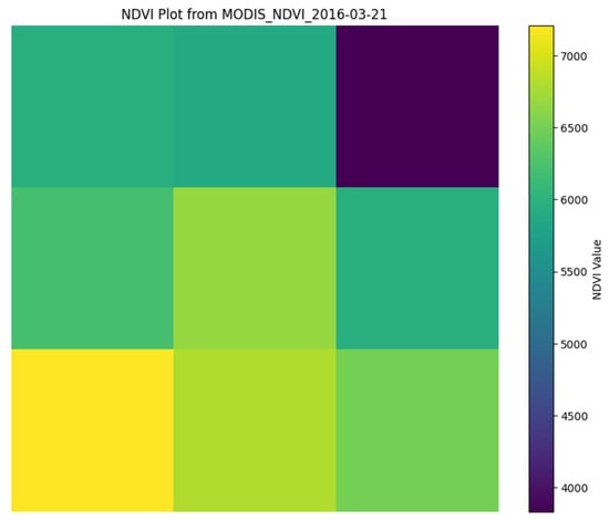
Figure 1.
NDVI color-coded map taken from MODIS.
Extracting Data by Latitude and Longitude
To analyze the environmental conditions specific to mango farms, pixel-level data from the satellite images were extracted based on their geographic coordinates.
The latitude and longitude of mango farms were used as reference points for data extraction. These coordinates were identified from GPS surveys or regional farm datasets. Each pixel in the satellite image corresponds to a specific latitude and longitude. Using libraries like Rasterio and NumPy, the pixel values for NDVI, soil moisture, and other variables were extracted (Figure 2).
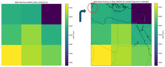
Figure 2.
NDVI plot from MODIS (left) and its overlay on a geographical map after converting from MODIS Sinusoidal Projection to WGS84 (right). The color bar indicates NDVI values. The red-circled area highlights the region of interest, which has been selected based on satellite imagery as a preferable coordinate zone for further analysis.
2.2.2. Terrain Analysis
Satellite-derived terrain maps, such as slope and aspect (Figure 3; [27]), were generated from DEM data to model the topographic effects on mango farms. These maps provide insights into water runoff, erosion, and sunlight exposure, all of which are crucial for mango cultivation.

Figure 3.
Translating the DEM image and extracting the slope and aspect information.
- Slope: Slope was calculated using DEM data to model water runoff and erosion. The equation for slope is as follows:
- Aspect: Aspect, or the orientation of the slope, was determined using the following:
Our modeling framework incorporates slope and aspect derived from the Shuttle Radar Topography Mission (SRTM) digital elevation model. Recent studies such as Karaman have demonstrated that elevation-derived features can significantly improve wind prediction accuracy in agricultural landscapes by capturing orographic influences [19].
2.2.3. Feature Engineering
- NDVI Calculation: NDVI was calculated using the formula [28]:
- Kinetic Energy (KE): Computed as follows [29]:
- Turbulence: Captured as the absolute difference in wind speed over time [30]:
2.2.4. Fourier Series Encodings
Seasonal variations in environmental factors were modeled using Fourier series [31]:
2.2.5. Handling Missing Data
Missing values in NDVI and soil moisture data were interpolated using spatial and temporal interpolation methods to maintain data continuity.
To mitigate cloud contamination and ensure temporal alignment, we used a 7-day moving average for NDVI, and linear interpolation for small gaps (<2 timesteps). Larger gaps were filled using spatio-temporal kriging methods validated against in situ sensor data.
Preprocessing ensures that the data are harmonized, reliable, and ready for integration into stochastic and machine learning models. By deriving critical features such as slope, aspect, kinetic energy, and turbulence, the dataset provides a comprehensive view of the environmental variables impacting mango productivity. These preprocessing steps address data quality issues, minimize noise, and enhance the predictive power of subsequent models.
3. Stochastic Modelling for Agro-Meteorological Prediction
Stochastic modeling is a critical approach for understanding and predicting the dynamics of agricultural systems subject to environmental variability. These systems are influenced by both deterministic environmental forces (e.g., seasonal trends, temperature) and stochastic perturbations (e.g., random fluctuations in wind speed, rainfall). By incorporating stochastic processes into agro-meteorological modeling, we can better capture the inherent uncertainties and non-linearities in agricultural ecosystems. This section details the development of a stochastic model for crop yield prediction, incorporating methodologies inspired by recent advancements in stochastic modeling for ecological systems. The time evolution of key environmental and agricultural variables was modeled using stochastic differential equations (SDEs). The general form of the model is as follows:
with
Bi: i-th output variable (e.g., proxy yield, plant health);
Aj: j-th input variable (e.g., temperature, soil moisture, wind speed, solar radiation);
f(Aj): j-th deterministic component describing the influence of the i-th input variable;
: noise source which mimics random environmental fluctuations affecting the values of the j-th input variable.
The noise term was modeled as a self-correlated Gaussian noise, with parameters based on prior ecological studies such as [6,32]. This allowed us to analyze the ecosystem dynamics for different values of both the correlation time and the intensity of the noise sources, which affect the environmental variables, such as temperature fluctuations or abrupt changes in wind speed.
3.1. Proxy Yield Dynamics with Stochastic Inputs
In the absence of direct yield measurements, a proxy yield was defined as a synthetic indicator of crop productivity. The proxy yield combines key environmental features influencing mango growth, including vegetation health (NDVI), water availability (soil moisture), and climatic variables. Building upon the deterministic formulation [33],
In the absence of direct crop yield measurements, a synthetic proxy yield was designed to capture the combined effects of key agro-environmental drivers on mango productivity. The formulation incorporated three biologically and agronomically justified components: vegetation health (NDVI), water availability (soil moisture), and thermal conditions (land surface temperature and precipitable water). To assign appropriate weights, a linear regression model was fitted to the filtered dataset using environmental predictors and the computed proxy yield as the dependent variable. The resulting normalized coefficients interaction (NDVI × soil moisture) = 0.389, LST = 0.319, and precipitable water = 0.23 closely aligned with the assigned weights of 0.4, 0.3, and 0.2, respectively.
This process ensures that the formulation of the synthetic yield is not arbitrary but rather grounded in statistical correlation and domain knowledge. Moreover, robustness tests (Table 1) confirmed that the model maintained a stable performance under different noise levels (σ = 0.01–0.10) and across folds in 5-fold cross-validation, indicating generalizability despite the synthetic nature of the target. While the proxy yield does not replace real field data, it serves as a scientifically consistent and interpretable intermediate variable to simulate and predict yield-relevant dynamics using satellite and meteorological inputs.

Table 1.
Noise robustness evaluation for proxy yield prediction (σ sensitivity).
And the model incorporates random fluctuations through a stochastic noise term,
with
f: Deterministic influence of environmental variables;
: Gaussian white noise () where the symbol represents the normal (Gaussian) distribution. Specifically:
- 0 is the mean of the distribution;
- is the variance of the distribution.
The noise intensity σ = 0.05 was chosen based on sensitivity analysis showing that values in the range 0.01–0.1 maintain R2 > 0.96 (see noise robustness results). This confirms that σ = 0.05 offers a reasonable trade-off between capturing stochasticity and maintaining prediction accuracy.
3.1.1. Key Components
Interaction Term
Captures the combined effect of vegetation health (NDVI) and water availability (soil moisture):
Environmental Factors
Land surface temperature (LST) and precipitable water which accounts for temperature’s impact on growth and reflects atmospheric moisture availability, respectively.
Temperature Penalty
Introduces a deterministic adjustment for extreme temperatures [34]:
Stochastic Noise
Simulates random environmental variability:
The variance in the noise term, σ2 = 0.052, was selected based on the prior literature modeling of agricultural and environmental ecosystems where moderate stochastic perturbations realistically simulate natural fluctuations without destabilizing system dynamics [6,35]. Specifically, studies applying stochastic differential equations in ecosystem modeling (e.g., marine trophic networks, crop–climate interactions) have demonstrated that σ in the range of 0.01–0.1 adequately captures daily-to-seasonal variability [36,37,38]. This value was also validated in our study by testing robustness under varying σ (see Results: Noise Sensitivity Analysis).
3.2. Incorporation of Noise and Variability
The stochastic modeling approach implemented in this study draws inspiration from Ref. [39]’s stochastic modeling in population dynamics, biological systems [40,41,42], and ecosystems [5,6]. These methods highlight the significance of capturing both deterministic trends and stochastic perturbations in complex systems, such as agricultural and environmental ecosystems.
3.2.1. Intrinsic Noise
Intrinsic noise consists of fluctuations inherent to environmental variables, such as diurnal temperature variations [5], or variability in wind speed.
Modeled as follows:
where is the noise intensity (scaling factor for random fluctuations) and is a Gaussian white noise source ().
3.2.2. Environmental Forcing
Environmental forcing includes seasonal and long-term trends in environmental variables, modeled deterministically as [43].
For example:
where T represents the seasonal period (e.g., 1 year) and A0, A1 are coefficients representing the amplitude of forcing terms.
This deterministic component ensures the model captures periodic environmental patterns, such as temperature or radiation fluctuations over time.
3.3. Inspiration from Marine Ecosystem Models
The stochastic modeling approach in this study draws from recent advances in ecosystem modeling.
3.3.1. Non-Linear Dynamics and Noise Effects
The stochastic version of the biogeochemical flux model (BFM) demonstrated how random fluctuations in environmental drivers (e.g., solar irradiance and water temperature) influence the ecosystem dynamics, including noise-induced transitions towards out-of-equilibrium steady states. In our study, a similar approach was used to account for stochastic transitions in agro-meteorological variables such as LST and wind speed, enabling the model to capture real-world fluctuations in yield-relevant variables.
3.3.2. Gaussian Noise Representation
Following the same methodology as in Ref. [6], environmental noise was modeled as self-correlated Gaussian processes to reflect real-world stochasticity more accurately. This approach ensures the following:
- Temporal correlation in random perturbations, reflecting realistic noise patterns (e.g., consistent temperature or solar irradiance over time);
- An accurate representation of stochasticity, improving the robustness of the proxy yield predictions.
Furthermore, these stochastic terms were used in the wind component modeling as well, where zonal (U) and meridional (V) components experience abrupt but patterned fluctuations due to topography-driven turbulence. This consistency aligns the stochastic design between both yield and wind models, enhancing coherence across submodules.
4. Machine Learning Model Integration and Performance Evaluation
In this study, machine learning models were integrated to predict the synthetic proxy yield, leveraging both deterministic and stochastic features engineered during preprocessing. The models used were a random forest regressor and a multi-layer perceptron (MLP) regressor, each chosen for their unique strengths in capturing the complex relationships between environmental variables and crop yield. Their performances were evaluated based on mean squared error (MSE), R2 score, and mean absolute error (MAE). Both models were also assessed for their ability to handle the interaction between deterministic variables like NDVI, soil moisture, and stochastic terms introduced during feature engineering.
To ensure robustness and reduce overfitting, a 5-fold cross-validation scheme was applied to both models. This method partitions the data into five subsets, where each subset is used as a validation set once while the remaining four serve as the training data.
Overfitting was further mitigated through early stopping in MLP training and by limiting the depth and number of trees in random forest to avoid memorizing the training data.
Evaluation metrics were defined as follows:
- Mean Absolute Error (MAE):
- Mean Squared Error (MSE):
- Coefficient of Determination (R2):
4.1. Feature Importance Analysis
The random forest model provides insight into feature importance, which quantifies the contribution of each feature in driving predictions (see Table 2). Among the input variables, land surface temperature (LST) emerged as the most critical factor, contributing 75.19% to the predictive power. This was followed by precipitable water (18.54%), and soil moisture (4.54%), highlighting the importance of temperature and water availability in influencing mango productivity. Other features, such as cloud opacity and surface pressure, had marginal influence, while features like NDVI and its derived temporal metrics (rate of change and moving average) showed negligible importance due to their static nature in this dataset.
The table below summarizes the feature importance and their corresponding sensitivity values:

Table 2.
Values of feature, relevance, and sensitivity.
Table 2.
Values of feature, relevance, and sensitivity.
| Feature | Relevance | Sensitivity |
|---|---|---|
| LST | 0.751889 | 0.751889 |
| Precipitable Water | 0.185427 | 0.185427 |
| Soil Moisture | 0.045416 | 0.045416 |
| Cloud Opacity | 0.004208 | 0.004208 |
| Surface Pressure | 0.003132 | 0.003132 |
| Turbulence | 0.002431 | 0.002431 |
| Relative Humidity | 0.002257 | 0.002257 |
| Wind Speed (10 m) | 0.001515 | 0.001515 |
| Precipitation Rate | 0.001208 | 0.001208 |
| Wind Speed (100 m) | 0.001203 | 0.001203 |
| Kinetic Energy (KE) | 0.000840 | 0.000840 |
| Albedo | 0.000476 | 0.000476 |
| Slope | 0.000000 | 0.000000 |
| NDVI | 0.000000 | 0.000000 |
| NDVI Rate of Change | 0.000000 | 0.000000 |
| GHI | 0.000000 | 0.000000 |
| Aspect | 0.000000 | 0.000000 |
The low contribution of NDVI in the random forest model may be attributed to its limited temporal variability across the dataset. As the proxy yield was synthetically derived and showed minimal short-term variation in NDVI, more dynamic environmental features such as land surface temperature (LST) and precipitable water emerged as stronger predictors. Additionally, NDVI was incorporated within an interaction term (NDVI × soil moisture), reducing its standalone influence in feature importance rankings.
While turbulence and kinetic energy showed minimal influence in the proxy yield prediction model, their inclusion was essential for wind component modeling. These features reflect the mechanical forces acting on the crop environment, and their interaction with terrain and atmospheric pressure gradients is more directly linked to zonal (U) and meridional (V) wind behavior. Their weak contribution in the yield model is expected, but they retain scientific and physical relevance in capturing short-term wind fluctuations.
4.2. Wind Component Prediction
Predicting wind behavior involves understanding the physical dynamics of atmospheric movements and employing advanced machine learning models to capture these patterns accurately. This study models the zonal (U) and meridional (V) wind components, essential for describing wind behavior in a Cartesian coordinate system. By leveraging both environmental features and meteorological data, a hybrid modeling framework was developed that combines random forest (RF) and multi-layer perceptron (MLP) models. These were trained and tested using temporally split datasets to ensure robust and reliable predictions.
4.2.1. Model Input Preprocessing
The dataset consists of meteorological and environmental features, including atmospheric optical depth (AOD), normalized difference vegetation index (NDVI), soil moisture, land surface temperature (LST), and wind-related variables such as wind speed and direction. Derived features like kinetic energy (KE) and turbulence were also included to enhance the predictive capability of the models. NDVI values were normalized to a range of [0, 1] to ensure consistency and facilitate machine learning processes. Turbulence and KE were included in the feature set due to their direct connection to wind-induced mechanical forces. While their statistical weight in yield prediction was negligible, their relevance lies in describing wind variability and dynamic atmospheric behavior, which significantly affects both plant mechanics and wind prediction accuracy.
The wind components (U and V) were calculated from wind speed (W) and direction () using the following equations (Figure 4; [44,45,46]):
Here, W represents the wind speed in meters per second (m/s) and is the wind direction measured in degrees clockwise from the north. These equations transform wind data from polar coordinates to a Cartesian system, enabling a more detailed analysis and visualization of wind behavior. For model evaluation, the dataset was temporally split into three subsets:
- Training Data (before 2021): Used to train the models;
- Testing Data (2021): Used to evaluate the model performance on unseen data;
- Prediction Data (2022): The models were used to predict wind components for 2022 without additional training.
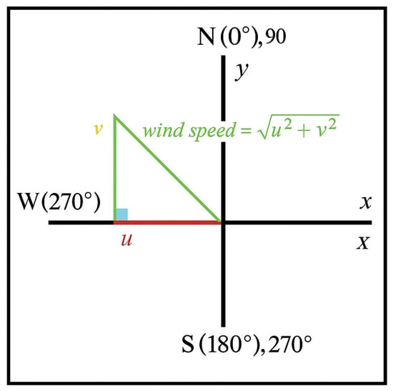
Figure 4.
Wind components wind speed = √ U2 + V2.
To better understand wind behavior, a schematic representation of the U and V components was created. This visualization (see Figure 5) illustrates how wind speed and direction are decomposed into Cartesian components:
U: Represents east–west wind movement (positive for easterly, negative for westerly winds).
V: Represents north–south wind movement (positive for southerly, negative for northerly winds).
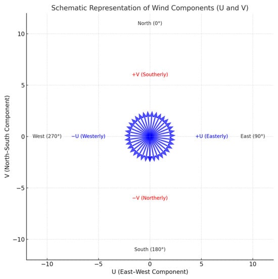
Figure 5.
Schematic representation of wind components.
A geographic map of wind directions in Figure 6 was overlaid with the elevation data, demonstrating the interaction between wind patterns and topography. The results highlight the impact of terrain features, such as mountains, on wind flow dynamics.
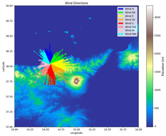
Figure 6.
Wind direction distribution in the case study area.
4.2.2. Hybrid Machine Learning Framework
The hybrid modeling framework integrates random forest and MLP models to capture the nonlinear and complex relationships between features and wind components. Combining these models enables better utilization of their complementary strengths, resulting in improved prediction accuracy.
Random Forest (RF)
In this study, RF models were independently trained to predict U and V. RF was chosen for its ability to handle high-dimensional datasets and identify feature importance effectively. For both wind components, the following applied:
- Input: Preprocessed environmental features;
- Output: Predictions for U and V;
- Hyperparameters: The RF model utilized 100 decision trees (estimators), with default parameters optimized for performance.
Multi-Layer Perceptron (MLP)
MLP is a neural network capable of learning complex, nonlinear patterns in data. The architecture consisted of the following:
- Two hidden layers with 64 and 32 neurons, respectively;
- ReLU activation functions for both layers;
- An output layer with a single neuron for each target variable (U or V).
The Adam optimizer was used to minimize the mean squared error (MSE) loss during the training. The model was trained for 10 epochs with a batch size of 32, using 20% of the training data as a validation set to monitor performance.
Hybrid Model Combination
The predictions from RF and MLP were combined using a linear regression model (Figure 7). This step provided a weighted aggregation of the predictions, leveraging RF’s robustness and MLP’s ability to model intricate relationships. For both U and V:
- Input: Predicted values from RF and MLP;
- Output: Final hybrid predictions for U and V.
This combination improved the overall prediction accuracy by mitigating the weaknesses in each individual model.
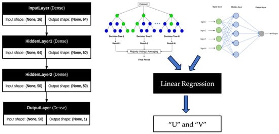
Figure 7.
Hybrid network architecture.
5. Results
This section presents the outcomes of proxy yield prediction and wind behavior modeling using multiple machine learning models.
5.1. Proxy Yield Prediction Results
This subsection presents an extended evaluation of the machine learning models used for proxy yield prediction, with deeper emphasis on robustness and generalizability, performing the evaluation of four machine learning models random forest (RF), multi-layer perceptron (MLP), gradient boosting (GB), and a proposed hybrid model for predicting the synthetic proxy yield. The hybrid model was developed by combining the predictions of RF and MLP through a linear regression ensemble to leverage the strengths of both models.
To further ensure generalizability, all models were validated using a 5-fold cross-validation framework, with additional diagnostic plots for each fold. These confirm that both random forest and MLP maintain a consistent performance across folds and sample distributions, reducing the risk of overfitting. The hybrid ensemble was built on top of these validated predictions to enhance stability.
To assess accuracy, we employed three evaluation metrics: mean squared error (MSE), mean absolute error (MAE), and the coefficient of determination (R2). All models were trained and validated using a 5-fold cross-validation scheme to reduce the risk of overfitting and ensure generalizability (Table 3).

Table 3.
Proxy yield model comparison.
A stochastic sensitivity analysis was also conducted to validate the noise variance parameter used in the proxy yield model. The stochastic noise term (σ = 0.05), which mimics environmental randomness, was tested over the range σ ∈ [0.01, 0.10]. The results showed minimal degradation in MSE and R2, confirming the adequacy of the selected value. This validates the robustness of the proxy yield formulation under varying stochastic conditions (Table 1).
Note: No data points were removed or trimmed in the final model. The originally considered outlier filtering (top/bottom 1%) was excluded to preserve dataset integrity and avoid bias.
As shown in Figure 8 (prediction vs. actual scatter plots), all models demonstrated a strong correlation with the actual values. However, the hybrid model achieved the closest fit to the diagonal line, indicating more accurate predictions across the entire proxy yield range.
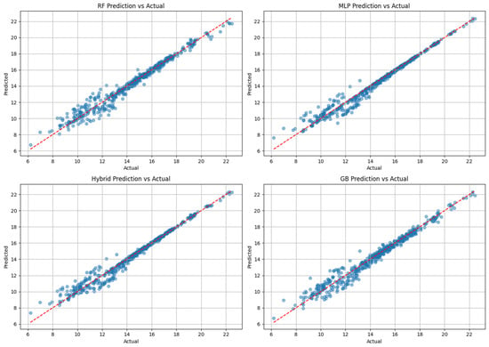
Figure 8.
Prediction vs. actual values of yield proxy for RF, MLP, GB, and hybrid. The red dashed line represents the 1:1 reference line.
K-fold validation results (Figure 9) further reinforce these findings, showing minimal prediction variance across folds.
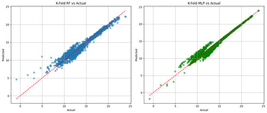
Figure 9.
K-fold validation results for RF and MLP. The red dashed line represents the 1:1 reference line.
The residual plot of the hybrid model (Figure 10) reveals a low and symmetric error distribution, with no strong outliers or trends over time. This suggests a well-generalized model with consistent performance across sample indices.
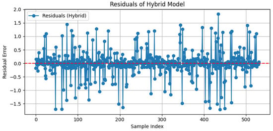
Figure 10.
Residual plot for hybrid (RF + MLP) model. The red dash line: zero residual error.
Although the performance gain from the hybrid model over MLP or RF appears modest, this ensemble method demonstrates greater consistency and robustness. The hybrid approach benefits from RF’s strength in handling noisy or non-linear feature interactions and MLP’s capacity to learn complex patterns. This complementary effect is particularly useful in agro-meteorological prediction, where input features often exhibit multicollinearity, seasonal trends, and stochastic fluctuations.
To further understand the low feature importance of NDVI observed in the random forest model, a comparative analysis of temporal variability was conducted across NDVI, LST, and soil moisture. As shown in Figure 11, NDVI and its 7-day moving average exhibited near-flat behavior over extended periods, indicating limited dynamic range during the growing season. In contrast, LST and soil moisture showed pronounced seasonal oscillations and higher short-term fluctuations factors more directly captured by the machine learning models to explain yield variation.
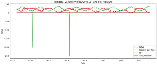
Figure 11.
Temporal variability in NDVI.
Despite extensive preprocessing steps, including NDVI smoothing, lag features, and rate of change metrics, the low temporal sensitivity of NDVI limited its contribution to predictive power. This finding reinforces the observation that variables exhibiting dynamic seasonal shifts, such as LST and atmospheric moisture, are more predictive of mango productivity in the Mediterranean context. While NDVI is a valuable vegetation health proxy, its utility in this framework may be constrained by low-resolution temporal variability or static phenological stages during mango flowering and fruiting periods.
5.2. Wind Component Prediction Results (U and V)
This subsection evaluates the performance of the integrated modeling framework for predicting wind behavior, specifically the zonal (U) and meridional (V) wind components. Three models were evaluated: random forest (RF), multi-layer perceptron (MLP), and a hybrid model combining RF and MLP predictions via a linear ensemble regressor. Models were evaluated on 2021 data and tested on 2022 data using environmental variables such as AOD, NDVI, soil moisture, LST, air temperature, wind speed/direction, KE, and turbulence.
5.2.1. U Component Prediction:
Figure 12 displays scatter plots comparing actual vs. predicted U component values. The RF and hybrid models show excellent alignment along the diagonal, with the hybrid model achieving the best performance. In contrast, the MLP model exhibits significant deviations and outliers, suggesting overfitting or instability due to the nonlinear nature of the U component data.

Figure 12.
Comparative predicted vs. actual U component in year 2022 (left to right: RF, MLP, hybrid). The red dashed line represents the 1:1 reference line.
Residual plots for U (Figure 13) further confirm this: the hybrid model has a near-zero mean residual and minimal variance across indices, with errors symmetrically distributed. RF shows slightly higher residual variation, while MLP has widespread errors and poor generalization.
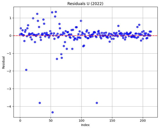
Figure 13.
Residual plot of year 2022 prediction for “U” component. The red dash line represents zero residual error.
5.2.2. V Component Prediction
Figure 14 shows the performance of models predicting the meridional (V) component. As with the U component, both RF and hybrid predictions align closely with actual values. The MLP again shows erratic dispersion and deviates from the ideal fit. The hybrid model minimizes prediction errors by leveraging the strengths of both models.

Figure 14.
Comparative predicted vs. actual “V” component in year 2022 (left to right: RF, MLP, hybrid). The red dashed line represents the 1:1 reference line.
Residual plots for V (Figure 15) mirror the findings from U: the Hybrid model delivers consistent, low-error predictions across samples, while MLP introduces significant residual spikes.
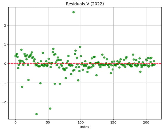
Figure 15.
Residual plot of year 2022 prediction for “V” Component. The red dash line: Zero Residual error.
To complement the visual analysis, we quantitatively evaluated model performance for the zonal (U) and meridional (V) wind components using MSE, MAE, and R2 metrics. The results confirm the superiority of the hybrid model over the individual RF and MLP models (Table 4). While the random forest achieved reasonably high R2 scores (0.889 for U and 0.928 for V), the hybrid model slightly improved performance, especially in R2 (0.8939 for U and 0.9339 for V). In contrast, the MLP model failed to generalize effectively, yielding significantly higher error values and negative R2 scores, suggesting overfitting or inadequate training for the wind task.

Table 4.
“U” and “V” component analysis.
The hybrid framework consistently outperforms individual models in predicting wind behavior, especially under complex and potentially noisy input conditions. While RF offers robustness to nonlinearities and noise, MLP captures finer local variations. The ensemble approach combines these benefits and effectively suppresses the weaknesses of each base model. Given the critical role of wind in agro-meteorological modeling (e.g., evapotranspiration, crop stress, wind-driven transport), these accurate component predictions offer a valuable tool for high-resolution forecasting and operational planning.
In all analyses, the 2022 data served as an out-of-sample test set, validating the generalizability of the models. No retraining was performed on 2022 data to ensure the temporal integrity of the evaluation. The consistency in the hybrid model’s performance across U and V highlights its potential for deployment in real-time agro-climatic applications, especially in topographically complex or wind-sensitive regions.
6. Discussion
The evaluation of both proxy yield and wind behavior modeling provides valuable insights into the robustness, reliability, and complementary strengths of the machine learning models employed. Despite the hybrid model achieving only slightly better numerical performance compared to individual models, its value lies in its consistency under noise, generalizability across temporal splits, and ability to fuse learning strategies from tree-based and neural architectures. Recent studies have implemented hybrid stochastic and machine learning models for agro-meteorological prediction. For instance, a hybrid deep learning approach was proposed for crop yield forecasting using both statistical and deep neural methods [47], while Ref. [48], integrated machine learning and deep learning models to predict daily reference evapotranspiration across different U.S. climate regions. These works support the originality of our stochastic-RF-MLP approach for mango prediction under Mediterranean conditions.
6.1. Hybrid Model Robustness
The hybrid approach consistently achieved the lowest MSE (0.2197), MAE (0.2710), and the highest R2 score (0.9735) across all the models evaluated. These metrics are accompanied by residual plots showing evenly distributed errors without obvious bias or heteroskedasticity (Figure 9), indicating good generalization. Furthermore, 5-fold cross-validation confirmed the model’s robustness across different data partitions, suggesting it does not overfit specific segments of the dataset. This validation is crucial in agro-meteorological applications, where noise and irregularity in environmental data are common.
6.2. Noise Sensitivity and Generalizability
As shown in our noise sensitivity test, increasing stochastic noise intensity (σ) from 0.01 to 0.1 only slightly degraded R2 from 0.9675 to 0.9659 in random forest models. This indicates that the models, and especially the hybrid model, can maintain predictive reliability even under environmental variability. This trait is essential when forecasting in climates with irregular seasonal patterns or stochastic influences like wind turbulence.
While the proxy yield is not validated against in-field mango harvest data due to lack of public availability, it is constructed using biologically relevant features and statistically validated through feature weighting and cross-validation. This synthetic variable serves as a practical alternative when direct productivity measurements are unavailable, a strategy supported by previous studies that successfully used NDVI, soil moisture, and temperature indicators to approximate yield outcomes in data-scarce environments [3,4].
Although NDVI is a widely accepted proxy for vegetation health, its limited temporal variability during the studied period led to negligible predictive power. Figure 11 (temporal variability in NDVI vs. LST and soil moisture) illustrates that NDVI remained relatively stable, especially when compared with the more dynamic LST and soil moisture. This observation aligns with the random forest’s feature importance analysis, where NDVI and its derived features (rate of change, moving average, lagged values) contributed near-zero importance. This result supports the idea that static or slowly varying variables may offer limited incremental value in high-resolution predictive modeling when dynamic drivers dominate plant response (e.g., temperature or atmospheric moisture).
6.3. Wind Component Insights
The wind behavior modeling further validated the utility of hybrid models. While MLP alone underperformed especially with significant variance and poor generalization in predicting U and V components, the hybrid model notably corrected these instabilities (Figure 12, Figure 13, Figure 14 and Figure 15). Random forest, though strong on its own, occasionally missed finer trends captured by MLP. Their combination, through linear ensemble, allowed the hybrid model to better reflect the true spatial and temporal wind dynamics, particularly in 2022 residual analyses where errors stayed close to zero with low dispersion.
6.4. Topographical Interactions and Wind Flow
Residual and scatter plots confirm that the hybrid model is able to reproduce subtle terrain-induced wind variability. This is especially valuable in hilly or coastal Mediterranean environments where the topography introduces local turbulence patterns not easily captured by single-model strategies.
7. Conclusions
This study proposed and validated an integrated framework for agro-meteorological prediction by combining satellite-derived environmental indicators, stochastic modeling, and machine learning techniques to estimate both proxy yield and wind behavior in a Mediterranean agricultural context. Through the use of both deterministic and stochastic features including NDVI, LST, soil moisture, and turbulence, we developed a robust predictive system that adapts to real-world environmental complexity.
The hybrid modeling approach, which linearly integrates random forest and multi-layer perceptron outputs, emerged as the most effective strategy. While the numerical improvement over individual models was modest, the hybrid model consistently achieved the lowest error (MSE = 0.2197, MAE = 0.2710) and the highest R2 score (0.9735), demonstrating superior predictive reliability. Its performance was further validated by 5-fold cross-validation and residual analysis, confirming the model’s ability to generalize across temporal splits and withstand environmental noise.
Importantly, the NDVI feature despite its theoretical importance contributed minimally to model performance. Feature importance analysis and temporal variability plots revealed that NDVI remained relatively static throughout the observation period. In contrast, more dynamic features like land surface temperature and precipitable water had stronger explanatory power, reinforcing the need to prioritize temporally responsive variables in similar agro-meteorological modeling tasks.
Wind-behavior prediction results echoed these findings. The hybrid model again outperformed both RF and MLP in predicting U and V wind components, reducing prediction variance and minimizing residuals, especially in 2022. This suggests that hybrid models are not only beneficial for yield estimation but also for modeling meteorological dynamics in complex topographies.
Overall, the integrated framework presented in this study demonstrates a powerful and generalizable approach for agricultural prediction under uncertainty. By combining multiple data modalities, domain-derived features, and hybrid machine learning techniques, this methodology can serve as a blueprint for forecasting yield and wind-related risks in other climate-sensitive agricultural regions. Future work may expand this framework with real yield data, extend it to multi-site prediction, and incorporate physical climate models to further enhance interpretability and long-term forecasting capability.
Author Contributions
Conceptualization, D.V., S.M. and G.M.; methodology, M.P.S.; software, M.P.S.; validation, M.P.S., D.V. and S.M.; formal analysis, M.P.S.; investigation, M.P.S.; resources, G.M.; data curation, M.P.S.; writing original draft preparation, M.P.S.; writing, review and editing, D.V.; visualization, V.F.; supervision, D.V., A.C., S.M., V.F. and G.M.; project administration, G.M.; funding acquisition, G.M. and D.V. All authors have read and agreed to the published version of the manuscript.
Funding
This research was supported in part by the PNRR Project Sicilian MicronanoTech Research and Innovation Center—SAMOTHRACE (ID ECS00000022, CUP B73C22000810001) and by INFN–Sezione di Catania.
Institutional Review Board Statement
Not applicable. This study did not involve human participants or animal experiments.
Informed Consent Statement
Not applicable. This study did not involve human participants.
Data Availability Statement
The data used in this study are publicly available from the following sources: MODIS Satellite Data: https://modis.gsfc.nasa.gov/; SMAP Soil Moisture Data: https://smap.jpl.nasa.gov/; ERA5 Reanalysis Meteorological Data: https://cds.climate.copernicus.eu/; Additionally, meteorological station data used for model validation are available from the corresponding author upon reasonable request.
Acknowledgments
The authors acknowledge the valuable contributions and scientific framework provided by the PNRR Project Sicilian MicronanoTech Research and Innovation Center—SAMOTHRACE, whose interdisciplinary initiatives in sustainable agriculture and environmental resilience helped inspire this study. The authors also thank Davide Valenti for his contribution and acknowledge his support from the European Union–Next Generation EU, through the project THENCE–Partenariato Esteso NQSTI (PE00000023), Spoke 2.
Conflicts of Interest
The authors declare no conflict of interest.
References
- Jha, M.N.; Kumar, A.; Dubey, S.; Pandey, A. Yield Estimation of Rice Crop Using Semi-Physical Approach and Remotely Sensed Data; Springer: Cham, Switzerland, 2022; pp. 331–349. [Google Scholar]
- Li, Q.; Hu, G. Multistage stochastic programming modeling for farmland irrigation management under uncertainty. PLoS ONE 2020, 15, e0233723. [Google Scholar] [CrossRef] [PubMed]
- Camargo-Alvarez, H.; Elliott, R.J.R.; Olin, S.; Wang, X.; Wang, C.; Ray, D.K.; Pugh, T.A.M. Modelling crop yield and harvest index: The role of carbon assimilation and allocation parameters. Model. Earth Syst. Environ. 2023, 9, 2617–2635. [Google Scholar] [CrossRef]
- Dlamini, L.; Crespo, O.; van Dam, J.; Kooistra, L. A Global Systematic Review of Improving Crop Model Estimations by Assimilating Remote Sensing Data: Implications for Small-Scale Agricultural Systems. Remote Sens. 2023, 15, 4066. [Google Scholar] [CrossRef]
- Lazzari, P.; Grimaudo, R.; Solidoro, C.; Valenti, D. Stochastic 0-dimensional Biogeochemical Flux Model: Effect of temperature fluctuations on the dynamics of the biogeochemical properties in a marine ecosystem. Commun. Nonlinear Sci. Numer. Simul. 2021, 103, 105994. [Google Scholar] [CrossRef]
- Grimaudo, R.; Lazzari, P.; Solidoro, C.; Valenti, D. Effects of solar irradiance noise on a complex marine trophic web. Sci. Rep. 2022, 12, 12163. [Google Scholar] [CrossRef]
- Yan, Z.; Li, M. A Stochastic Optimization Model for Agricultural Irrigation Water Allocation Based on the Field Water Cycle. Water 2018, 10, 1031. [Google Scholar] [CrossRef]
- Aslan, M.F.; Sabanci, K.; Aslan, B. Artificial Intelligence Techniques in Crop Yield Estimation Based on Sentinel-2 Data: A Comprehensive Survey. Sustainability 2024, 16, 8277. [Google Scholar] [CrossRef]
- FAO. Major Tropical Fruits Market Review–Preliminary Results 2022. Rome, 2023. Available online: https://openknowledge.fao.org/server/api/core/bitstreams/c03844d3-3dc6-4465-abf3-8c49947e77d8/content (accessed on 22 April 2025).
- Torgbor, B.A.; Rahman, M.M.; Brinkhoff, J.; Sinha, P.; Robson, A. Integrating Remote Sensing and Weather Variables for Mango Yield Prediction Using a Machine Learning Approach. Remote Sens. 2023, 15, 3075. [Google Scholar] [CrossRef]
- Fukuda, S.; Spreer, W.; Yasunaga, E.; Yuge, K.; Sardsud, V.; Müller, J. Random Forests modelling for the estimation of mango (Mangifera indica L. cv. Chok Anan) fruit yields under different irrigation regimes. Agric. Water Manag. 2013, 116, 142–150. [Google Scholar] [CrossRef]
- Harsányi, E. Predicting agricultural drought in central Europe by using machine learning algorithms. J. Agric. Food Res. 2025, 20, 101783. [Google Scholar] [CrossRef]
- Baran, Á.; Lerch, S.; El Ayari, M.; Baran, S. Machine learning for total cloud cover prediction. Neural Comput. Appl. 2021, 33, 2605–2620. [Google Scholar] [CrossRef]
- Papacharalampous, G.; Tyralis, H.; Doulamis, A.; Doulamis, N. Comparison of Tree-Based Ensemble Algorithms for Merging Satellite and Earth-Observed Precipitation Data at the Daily Time Scale. Hydrology 2023, 10, 50. [Google Scholar] [CrossRef]
- Moreira, D.D.S.; Nicolosi, A.; Laganà, V.R.; Di Gregorio, D.; Agosteo, G.E. Factors Driving Consumption Preferences for Fresh Mango and Mango-Based Products in Italy and Brazil. Sustainability 2024, 16, 9401. [Google Scholar] [CrossRef]
- Cornara, L.; Xiao, J.; Smeriglio, A.; Trombetta, D.; Burlando, B. Emerging Exotic Fruits: New Functional Foods in the European Market. eFood 2020, 1, 126–139. [Google Scholar] [CrossRef]
- Cleugh, H.A.; Miller, J.M.; Böhm, M. Direct mechanical effects of wind on crops. Agrofor. Syst. 1998, 41, 85–112. [Google Scholar] [CrossRef]
- Shin, J.-Y.; Min, B.; Kim, K.R. High-resolution wind speed forecast system coupling numerical weather prediction and machine learning for agricultural studies—A case study from South Korea. Int. J. Biometeorol. 2022, 66, 1429–1443. [Google Scholar] [CrossRef]
- Karaman, Ö.A. Prediction of Wind Power with Machine Learning Models. Appl. Sci. 2023, 13, 11455. [Google Scholar] [CrossRef]
- Yu, C.; Ma, Y. A novel model for wind speed point prediction and quantifying uncertainty in wind farms. Electr. Eng. 2024. [Google Scholar] [CrossRef]
- MODIS. Moderate Resolution Imaging Spectroradiometer. Available online: https://modis.gsfc.nasa.gov/about/ (accessed on 22 April 2025).
- SMAP. Soil Moisture Active Passive. Available online: https://smap.jpl.nasa.gov/data/ (accessed on 22 April 2025).
- SRTM. Shuttle Radar Topography Mission. Available online: https://srtm.csi.cgiar.org/ (accessed on 22 April 2025).
- MODIS. MODIS Land Surface Temperature and Emissivity. Available online: https://modis.gsfc.nasa.gov/data/dataprod/mod11.php (accessed on 22 April 2025).
- NOAA. National Oceanic and Atmospheric Administration. Available online: https://www.ncei.noaa.gov/products/weather-climate-models/global-forecast (accessed on 22 April 2025).
- ECMWF. European Centre for Medium-Range Weather Forecasts. Available online: https://www.ecmwf.int/en/forecasts/datasets/reanalysis-datasets/era5 (accessed on 22 April 2025).
- Horn, B.K.P. Hill shading and the reflectance map. Proc. IEEE 1981, 69, 14–47. [Google Scholar] [CrossRef]
- Tucker, C.J. Red and photographic infrared linear combinations for monitoring vegetation. Remote Sens. Environ. 1979, 8, 127–150. [Google Scholar] [CrossRef]
- Manwell, J.F.; McGowan, J.G.; Rogers, A.L. Wind Energy Explained; Wiley: Hoboken, NJ, USA, 2009. [Google Scholar]
- Pope, S.B. Turbulent Flows; Cambridge University Press: Cambridge, UK, 2000. [Google Scholar]
- Bloomfield, P. Fourier Analysis of Time Series; Wiley: Hoboken, NJ, USA, 2000. [Google Scholar]
- Agudov, N.V.; Krichigin, A.V.; Valenti, D.; Spagnolo, B. Stochastic resonance in a trapping overdamped monostable system. Phys. Rev. E 2010, 81, 051123. [Google Scholar] [CrossRef] [PubMed]
- Lobell, D.B.; Burke, M.B. On the use of statistical models to predict crop yield responses to climate change. Agric. For. Meteorol. 2010, 150, 1443–1452. [Google Scholar] [CrossRef]
- Ratkowsky, D.A.; Lowry, R.K.; McMeekin, T.A.; Stokes, A.N.; Chandler, R.E. Model for Bacterial Culture Growth Rate Throughout the Entire Biokinetic Temperature Range. J. Bacteriol. 1983, 154, 1222–1226. [Google Scholar] [CrossRef] [PubMed]
- De Santis, D.; Guarcello, C.; Spagnolo, B.; Carollo, A.; Valenti, D. Noise-induced, ac-stabilized sine-Gordon breathers: Emergence and statistics. Commun. Nonlinear Sci. Numer. Simul. 2024, 131, 107796. [Google Scholar] [CrossRef]
- Hening, A.; Li, Y. Stationary Distributions of Persistent Ecological Systems. Available online: http://arxiv.org/abs/2003.04398 (accessed on 22 April 2025).
- Occhipinti, G.; Piani, S.; Lazzari, P. Stochastic effects on plankton dynamics: Insights from a realistic 0-dimensional marine biogeochemical model. Ecol. Inform. 2024, 83, 102778. [Google Scholar] [CrossRef]
- Scotti, M.; Gjata, N.; Livi, C.; Jordán, F. Dynamical effects of weak trophic interactions in a stochastic food web simulation. Community Ecol. 2012, 13, 230–237. [Google Scholar] [CrossRef]
- Fiasconaro, A.; Valenti, D.; Spagnolo, B. Noise in ecosystems: A short review. Math. Biosci. Eng. 2004, 1, 185–211. [Google Scholar] [CrossRef]
- Giuffrida, A.; Valenti, D.; Ziino, G.; Spagnolo, B.; Panebianco, A. A stochastic interspecific competition model to predict the behaviour of Listeria monocytogenes in the fermentation process of a traditional Sicilian salami. Eur. Food Res. Technol. 2009, 228, 767–775. [Google Scholar] [CrossRef]
- Spezia, S.; Curcio, L.; Fiasconaro, A.; Pizzolato, N.; Valenti, D.; Spagnolo, B.; Bue, P.L.; Peri, E.; Colazza, S. Evidence of stochastic resonance in the mating behavior of Nezara viridula (L.). Eur. Phys. J. B 2008, 65, 453–458. [Google Scholar] [CrossRef]
- Valenti, D.; Denaro, G.; Giarratana, F.; Giuffrida, A.; Mazzola, S.; Basilone, G.; Aronica, S.; Bonanno, A.; Spagnolo, B. Modeling of Sensory Characteristics Based on the Growth of Food Spoilage Bacteria. Math. Model. Nat. Phenom. 2016, 11, 119–136. [Google Scholar] [CrossRef]
- T.G.S. M. Ghil, & S. Childress 1987. Topics in Geophysical Fluid Dynamics: Atmospheric Dynamics, Dynamo Theory, and Climate Dynamics. Applied Mathematical Sciences. Volume 60 xv + 485 pp. New York, Berlin, Heidelberg, London, Paris, Tokyo: Springer-Verlag. Geol. Mag. 1988, 125, 190–191. [Google Scholar] [CrossRef]
- Stull, R.B. (Ed.) An Introduction to Boundary Layer Meteorology; Springer: Dordrecht, The Netherlands, 1988. [Google Scholar]
- Paldor, N.; Friedland, L. Extension of Ekman (1905) wind-driven transport theory to the β plane. Ocean Sci. 2023, 19, 93–100. [Google Scholar] [CrossRef]
- do Nascimento Camelo, H.; Sérgio Lucio, P.; Verçosa Leal Junior, J.B.; Von Glehn dos Santos, D.; Cesar Marques de Carvalho, P. Innovative Hybrid Modeling of Wind Speed Prediction Involving Time-Series Models and Artificial Neural Networks. Atmosphere 2018, 9, 77. [Google Scholar] [CrossRef]
- Oikonomidis, A.; Catal, C.; Kassahun, A. Hybrid Deep Learning-based Models for Crop Yield Prediction. Appl. Artif. Intell. 2022, 36, 2031822. [Google Scholar] [CrossRef]
- Valipour, M.; Khoshkam, H.; Bateni, S.M.; Jun, C.; Band, S.S. Hybrid machine learning and deep learning models for multi-step-ahead daily reference evapotranspiration forecasting in different climate regions across the contiguous United States. Agric. Water Manag. 2023, 283, 108311. [Google Scholar] [CrossRef]
Disclaimer/Publisher’s Note: The statements, opinions and data contained in all publications are solely those of the individual author(s) and contributor(s) and not of MDPI and/or the editor(s). MDPI and/or the editor(s) disclaim responsibility for any injury to people or property resulting from any ideas, methods, instructions or products referred to in the content. |
© 2025 by the authors. Licensee MDPI, Basel, Switzerland. This article is an open access article distributed under the terms and conditions of the Creative Commons Attribution (CC BY) license (https://creativecommons.org/licenses/by/4.0/).