Article

The New Marshall–Olkin–Type II Exponentiated Half-Logistic–Odd Burr X-G Family of Distributions with Properties and Applications

by
Broderick Oluyede
1,*,
Thatayaone Moakofi
2 and
Gomolemo Lekono
1
1
Department of Mathematics and Statistical Sciences, Botswana International University of Science and Technology, Palapye 10071, Botswana
2
Independent Researcher, Botswana
*
Author to whom correspondence should be addressed.
Stats 2025, 8(2), 26; https://doi.org/10.3390/stats8020026
Submission received: 28 February 2025 / Revised: 28 March 2025 / Accepted: 3 April 2025 / Published: 4 April 2025

Abstract

:
We develop a novel family of distributions named the Marshall–Olkin type II exponentiated half-logistic–odd Burr X-G distribution. Several mathematical properties including linear representation of the density function, Rényi entropy, probability-weighted moments, and distribution of order statistics are obtained. Different estimation methods are employed to estimate the unknown parameters of the new distribution. A simulation study is conducted to assess the effectiveness of the estimation methods. A special model of the new distribution is used to show its usefulness in various disciplines.

1. Introduction

Some recent work in statistical distribution theory includes generating new and generalized distributions by introducing additional parameter(s) to existing distributions. This results in flexible and generalized distributions. There are different generators available in the literature. These include Marshall–Olkin-G by [1], odd Burr X-G by [2], Topp–Leone-G by [3], type II half-logistic-G by [4], type II exponentiated half-logistic-G by [5], gamma-G (type 1) by [6], and gamma-G (type 2) by [7].
Some examples of recently generalized families of distributions include Marshall–Olkin–Topp–Leone-G family of distributions by [8], Marshall–Olkin extended Burr type XII distribution by [9], Marshall–Olkin generalized-G family of distributions by [10], Marshall–Olkin Fréchet distribution by [11], Marshall–Olkin generalized exponential distribution by [12], Marshall–Olkin alpha power Weibull distribution by [13], Marshall–Olkin alpha power inverse exponential distribution by [14], Marshall–Olkin logistic exponential distribution by [15], type II exponentiated half-logistic–odd Burr X-G power series class of distributions by [16], and Topp–Leone–odd Burr X-G family of distributions by [17]. Other distributions available in the literature include a comparative analysis of Poisson regression-based mean estimators by [18] as well as a paper on combining ratio and product type estimators for estimation of the finite population mean in adaptive cluster sampling design by [19].
Marshall and Olkin [1] introduced a family of distributions called the Marshall–Olkin-G (MO-G) distribution with cumulative distribution function (cdf) and probability distribution function (pdf), given by
F M O G ( x ; δ , Ξ ) = 1 δ G ¯ ( x ; Ξ ) 1 ( 1 δ ) G ¯ ( x ; Ξ )
and
f M O G ( x ; δ , Ξ ) = δ g ( x ; Ξ ) [ 1 ( 1 δ ) G ¯ ( x ; Ξ ) ] 2 ,
respectively, for x , δ > 0 , where G ¯ ( x ; Ξ ) = 1 G ( x ; Ξ ) is the survival function of the baseline distribution with the cdf G ( x ; Ξ ) .
The type II exponentiated half-logistic-G (TIIEHL-G) was proposed by [5]. The cdf and pdf of the TIIEHL-G family of distributions are given by
F T I I E H L G ( x ; α , Ξ ) = 1 1 G ( x ; Ξ ) 1 + G ( x ; Ξ ) α
and
f T I I E H L G ( x ; α , Ξ ) = 2 α g ( x ; Ξ ) 1 G ( x ; Ξ ) α 1 1 + G ( x ; Ξ ) α + 1 ,
respectively, where α > 0 is the shape parameter, G ( x ; Ξ ) is the baseline cdf, and g ( x ; Ξ ) is the baseline pdf, which depends on the parameter vector Ξ .
The cdf and pdf of the odd Burr X-G (OBX-G) family of distributions (see [2]) are given by
F O B X G ( x ; β , Ξ ) = 1 exp G ( x ; Ξ ) G ¯ ( x ; Ξ ) 2 β
and
f O B X G ( x ; β , Ξ ) = 2 β g ( x ; Ξ ) G ( x ; Ξ ) G ¯ 3 ( x ; Ξ ) exp G ( x ; Ξ ) G ¯ ( x ; Ξ ) 2 × 1 exp G ( x ; Ξ ) G ¯ ( x ; Ξ ) 2 β 1 ,
respectively, for x , β > 0 , and parent cdf parameter vector Ξ .
In this paper, we introduce a new family of generalized distributions that exhibit diverse hazard rate functions (hrfs), encompassing both monotonic and non-monotonic shapes. The new family combines the MO-G, TIIEHL-G, and OBX-G families to obtain the new and generalized MO-TIIEHL-OBX-G distribution. Another motivation for developing the new family of distributions is the construction of distributions for modeling different real datasets, as well as distributions with symmetric, left-skewed, right-skewed, and reverse-J shapes. We also seek to develop a new family of distributions which provide better fits than other generated distributions under the same transformation, and the underlying baseline cdf. Merging distributions like Marshall–Olkin and exponentiated half-logistic increases flexibility, allowing better modeling of complex data with features such as skewness and heavy tails. This helps capture a wider range of behaviors, making the model more suitable for real-world data that a standard distribution might not fit well.
This paper is organized as follows. In Section 2, we introduce the new family of distributions and its sub-families. In Section 3, the mathematical properties of the new model are explored including the expansion of the pdf, quantile function, moments, generating function, and Rényi entropy. The parameter estimates are obtained using different estimation methods in Section 4. Some special cases of the new family of distributions are given in Section 4. A Monte Carlo simulation study is conducted in Section 5 to assess the bias and mean square error of the estimates. Key risk measures and numerical studies using them are given in Section 6. Section 7 gives applications of the new model to real datasets, and conclusions are given in Section 8.

2. The New Family of Distributions

We present the new family of distributions and its sub-families in this section. The Marshall–Olkin–type II exponentiated half-logistic-G–odd Burr X-G (MO-TIIEHL-OBX-G) family of distributions obtained by combining the families in Equations (1)–(6), the cdf and pdf of which are given by
F ( x ; δ , α , β , Ξ ) = 1 δ 1 1 exp G ( x ; Ξ ) G ¯ ( x ; Ξ ) 2 β 1 + 1 exp G ( x ; Ξ ) G ¯ ( x ; Ξ ) 2 β α 1 1 δ 1 1 exp G ( x ; Ξ ) G ¯ ( x ; Ξ ) 2 β 1 + 1 exp G ( x ; Ξ ) G ¯ ( x ; Ξ ) 2 β α ,
and
f ( x ; δ , α , β , Ξ ) = 4 δ α β G ( x ; Ξ ) g ( x ; Ξ ) G ¯ 3 ( x ; Ξ ) exp G ( x ; Ξ ) G ¯ ( x ; Ξ ) 2 1 exp G ( x ; Ξ ) G ¯ ( x ; Ξ ) 2 β 1 × 1 1 exp G ( x ; Ξ ) G ¯ ( x ; Ξ ) 2 β α 1 × 1 + 1 exp G ( x ; Ξ ) G ¯ ( x ; Ξ ) 2 β ( α + 1 ) × 1 1 δ 1 1 exp G ( x ; Ξ ) G ¯ ( x ; Ξ ) 2 β 1 + 1 exp G ( x ; Ξ ) G ¯ ( x ; Ξ ) 2 β α 2 ,
respectively, for δ , α , β > 0 , and parameter vector Ξ , where δ is the tilt parameter, and α and β are shape parameters.
The hazard rate function (hrf) is given by
h ( x ; δ , α , β , Ξ ) = 4 δ α β G ( x ; Ξ ) g ( x ; Ξ ) G ¯ 3 ( x ; Ξ ) exp G ( x ; Ξ ) G ¯ ( x ; Ξ ) 2 1 exp G ( x ; Ξ ) G ¯ ( x ; Ξ ) 2 β 1 × 1 1 exp G ( x ; Ξ ) G ¯ ( x ; Ξ ) 2 β α 1 × 1 + 1 exp G ( x ; Ξ ) G ¯ ( x ; Ξ ) 2 β ( α + 1 ) × 1 1 δ 1 1 exp G ( x ; Ξ ) G ¯ ( x ; Ξ ) 2 β 1 + 1 exp G ( x ; Ξ ) G ¯ ( x ; Ξ ) 2 β α 2 × δ 1 1 exp G ( x ; Ξ ) G ¯ ( x ; Ξ ) 2 β 1 + 1 exp G ( x ; Ξ ) G ¯ ( x ; Ξ ) 2 β α 1 1 δ 1 1 exp G ( x ; Ξ ) G ¯ ( x ; Ξ ) 2 β 1 + 1 exp G ( x ; Ξ ) G ¯ ( x ; Ξ ) 2 β α 1 ,
for δ , α , β > 0 , and parameter vector Ξ .

Sub-Families

Several new sub-families are presented in this subsection. These new sub-families show how diverse and consequential the MO-TIIEHL-OBX-G is in the framework of new and generalized families of distributions.
  • When α = 1 , we obtain the new Marshall–Olkin–type II half-logistic-G–odd Burr X-G (MO-TIIHL-OBX-G) family of distributions, with the cdf given by
    F ( x ; δ , β , Ξ ) = 1 δ 1 1 exp G ( x ; Ξ ) G ¯ ( x ; Ξ ) 2 β 1 + 1 exp G ( x ; Ξ ) G ¯ ( x ; Ξ ) 2 β 1 1 δ 1 1 exp G ( x ; Ξ ) G ¯ ( x ; Ξ ) 2 β 1 + 1 exp G ( x ; Ξ ) G ¯ ( x ; Ξ ) 2 β ,
    for δ , β > 0 , and parameter vector Ξ .
  • If δ = 1 , we obtain the type II exponentiated half-logistic-G odd Burrr X-G (TIIEHL-OBX-G) with the cdf given by
    F ( x ; α , β , Ξ ) = 1 1 1 exp G ( x ; Ξ ) G ¯ ( x ; Ξ ) 2 β 1 + 1 exp G ( x ; Ξ ) G ¯ ( x ; Ξ ) 2 β α ,
    for α , β > 0 , and parameter vector Ξ . This is a new family of distributions.
  • When β = 1 , we obtain the Marshall–Olkin–type II exponentiated half-logistic-G–odd Rayleigh-G (MO-TIIEHL-OR-G) family of distributions, with the cdf given by
    F ( x ; α , δ , Ξ ) = 1 δ exp G ( x ; Ξ ) G ¯ ( x ; Ξ ) 2 1 + 1 exp G ( x ; Ξ ) G ¯ ( x ; Ξ ) 2 α 1 1 δ exp G ( x ; Ξ ) G ¯ ( x ; Ξ ) 2 1 + 1 exp G ( x ; Ξ ) G ¯ ( x ; Ξ ) 2 α ,
    for α , δ > 0 , and parameter vector Ξ . This is a new family of distributions.
  • When α = β = 1 , we obtain the Marshall–Olkin–type II half-logistic-G–odd Rayleigh-G (MO-TIIHL-OR-G) family of distributions, with the cdf given by
    F ( x ; δ , Ξ ) = 1 δ exp G ( x ; Ξ ) G ¯ ( x ; Ξ ) 2 1 + 1 exp G ( x ; Ξ ) G ¯ ( x ; Ξ ) 2 1 1 δ exp G ( x ; Ξ ) G ¯ ( x ; Ξ ) 2 1 + 1 exp G ( x ; Ξ ) G ¯ ( x ; Ξ ) 2 ,
    for δ > 0 and parameter vector Ξ . This is a new family of distributions.
  • When α = δ = 1 , we obtain the type II half-logistic-G odd Burrr X-G (TIIHL-OBX-G) family of distributions, with the cdf given by
    F ( x ; β , Ξ ) = 1 1 1 exp G ( x ; Ξ ) G ¯ ( x ; Ξ ) 2 β 1 + 1 exp G ( x ; Ξ ) G ¯ ( x ; Ξ ) 2 β ,
    for β > 0 and parameter vector Ξ . This is a new family of distributions.
  • When β = δ = 1 , we obtain the type II exponentiated half-logistic-G Odd Rayleigh-G (TIIEHL-OR-G) family of distributions, with the cdf given by
    F ( x ; α , Ξ ) = 1 exp G ( x ; Ξ ) G ¯ ( x ; Ξ ) 2 1 + 1 exp G ( x ; Ξ ) G ¯ ( x ; Ξ ) 2 α ,
    for α > 0 and parameter vector Ξ . This is a new family of distributions.
  • When α = β = δ = 1 , we obtain the type II half-logistic-G Odd Rayleigh-G (TIIHL-OR-G) family of distributions, with the cdf given by
    F ( x ; Ξ ) = 1 exp G ( x ; Ξ ) G ¯ ( x ; Ξ ) 2 1 + 1 exp G ( x ; Ξ ) G ¯ ( x ; Ξ ) 2 ,
    with parameter vector Ξ . This is a new family of distributions.
    There are several generalized distributions that can be readily obtained by specifying the baseline cdf G.

3. Some Statistical Properties

The statistical properties of the MO-TIIEHL-OBX-G family of distributions are explored in this section. The statistical properties considered include expansion of the density function, quantile function, generating function, probability-weighted moments, Rényi entropy, and distribution of order statistics.

3.1. Linear Representation of the Density

Consider the generalized series expansion given by 1 z a = i = 0 ( 1 ) i a i z a ; for | z | < 1 , we can write
1 δ ¯ 1 1 exp G ( x ; Ξ ) G ¯ ( x ; Ξ ) 2 β 1 + 1 exp G ( x ; Ξ ) G ¯ ( x ; Ξ ) 2 β α 2 = i = 0 i + 1 i δ ¯ i × 1 1 exp G ( x ; Ξ ) G ¯ ( x ; Ξ ) 2 β 1 + 1 exp G ( x ; Ξ ) G ¯ ( x ; Ξ ) 2 β α i ,
1 1 exp G ( x ; Ξ ) G ¯ ( x ; Ξ ) 2 β α i + α 1 = j = 0 1 j α i + α 1 j × 1 exp G ( x ; Ξ ) G ¯ ( x ; Ξ ) 2 β j ,
1 + 1 exp G ( x ; Ξ ) G ¯ ( x ; Ξ ) 2 β ( α i + α + 1 ) = k = 0 1 k α i + α + k k × 1 exp G ( x ; Ξ ) G ¯ ( x ; Ξ ) 2 β k ,
1 exp G ( x ; Ξ ) G ¯ ( x ; Ξ ) 2 β ( k + j + 1 ) 1 = l = 0 1 l β ( k + j + 1 ) 1 l × exp l G ( x ; Ξ ) G ¯ ( x ; Ξ ) 2 ,
exp ( l + 1 ) G ( x ; Ξ ) G ¯ ( x ; Ξ ) 2 = m = 0 1 m l + 1 m G 2 m ( x ; Ξ ) m ! G ¯ 2 m ( x ; Ξ ) ,
1 G ( x ; Ξ ) ( 2 m + 3 ) = n = 0 2 m + n + 2 n G n ( x ; Ξ ) ,
1 G ¯ ( x ; Ξ ) n + 2 m + 1 = p = 0 1 p n + 2 m + 1 p G ¯ p ( x ; Ξ ) ,
1 G ( x ; Ξ ) p = q = 0 1 q p q G q ( x ; Ξ ) ,
and the pdf of the MO-TIIEHL-OBX-G can be written as
f ( x ; δ , α , β , Ξ ) = 4 δ α β i , j , k , l , m , n , p , q = 0 1 j + k + l + m + p + q i + 1 i α i + α 1 j × α i + α + k k β ( k + j + 1 ) 1 l 2 m + n + 2 n × n + 2 m + 1 p p q l + 1 m m ! δ ¯ i g ( x ; Ξ ) G q ( x ; Ξ ) = q = 0 ω q + 1 h q + 1 ( x ; Ξ ) ,
where
ω q + 1 = 4 δ α β q + 1 i , j , k , l , m , n , p = 0 1 j + k + l + m + p + q i + 1 i α i + α 1 j × α i + α + k k β k + β j + β 1 l 2 m + n + 2 n n + 2 m + 1 p × p q l + 1 m m ! δ ¯ i
and h q + 1 ( x ; Ξ ) = ( q + 1 ) g ( x ; Ξ ) G q ( x ; Ξ ) is the exponentiated-G (exp-G) density with power parameter (q + 1) and parameter vector Ξ . Hence, the density of MO-TIIEHL-OBX-G family of distributions can be expressed as an infinite linear combination of exp-G densities. As a result, the mathematical and statistical properties follow directly from those of the exp-G distributions.

3.2. Quantile Function

The quantile function of the MO-TIIEHL-OBX-G family of distributions is obtained by solving the non-linear equation
F ( x ; δ , α , β , Ξ ) = 1 δ 1 1 exp G ( x ; Ξ ) G ¯ ( x ; Ξ ) 2 β 1 + 1 exp G ( x ; Ξ ) G ¯ ( x ; Ξ ) 2 β α 1 1 δ 1 1 exp G ( x ; Ξ ) G ¯ ( x ; Ξ ) 2 β 1 + 1 exp G ( x ; Ξ ) G ¯ ( x ; Ξ ) 2 β α = u ,
0 u 1 . Note that Equation (12) can be written as
G ( x ; Ξ ) = log 1 1 1 u δ + ( 1 u ) δ ¯ 1 α 1 + 1 u δ + ( 1 u ) δ ¯ 1 α 1 β 1 2 1 + log 1 1 1 u δ + ( 1 u ) δ ¯ 1 α 1 + 1 u δ + ( 1 u ) δ ¯ 1 α 1 β 1 2 .
Consequently, the quantile function of the MO-TIIEHL-OBX-G family of distributions is given by
Q X ( u ; δ , α , β , Ξ ) = G 1 log 1 1 1 u δ + ( 1 u ) δ ¯ 1 α 1 + 1 u δ + ( 1 u ) δ ¯ 1 α 1 β 1 2 1 + log 1 1 1 u δ + ( 1 u ) δ ¯ 1 α 1 + 1 u δ + ( 1 u ) δ ¯ 1 α 1 β 1 2 .
As a result, Equation (13) can be used to generate random numbers from the MO-TIIEHL-OBX-G family of distributions for the specified baseline cdf G ( x ; Ξ ) .

3.3. Moments and Probability-Weighted Moments

The moments, moment-generating function, and probability-weighted moments (PWMs) of the MO-TIIEHL-OBX-G family of distributions are presented in this subsection. Using Equation (10), we obtain the rth moment of the MO-TIIEHL-OBX-G family of distribution as follows:
E ( X r ) = x r f M O T I I E H L O B X G ( x ; δ , α , β , Ξ ) d x = q = 0 ω q + 1 E ( Y q + 1 r ) ,
where E ( Y q + 1 r ) is the r t h moment of Y q + 1 , which follows the exp-G distribution with power parameter ( q + 1 ) and ω q + 1 is defined as Equation (11). The moment-generating function is given by
M X ( t ) = E ( e t X ) = q = 0 ω q + 1 E ( e t Y q + 1 ) ,
where E ( e t Y q + 1 ) is the moment-generating function of an exp-G distributed random variable Y q + 1 with power parameter ( q + 1 ), and ω q + 1 is given by Equation (11). The PWMs of a random variable X are defined by
ω a , r = E X a [ F ( X ) ] r = x a [ F ( x ) ] r f ( x ) d x .
Using the generalized binomial expansions
1 δ 1 1 exp G ( x ; Ξ ) G ¯ ( x ; Ξ ) 2 β 1 + 1 exp G ( x ; Ξ ) G ¯ ( x ; Ξ ) 2 β α 1 δ ¯ 1 1 exp G ( x ; Ξ ) G ¯ ( x ; Ξ ) 2 β 1 + 1 exp G ( x ; Ξ ) G ¯ ( x ; Ξ ) 2 β α r = i = 0 1 i r i δ i × 1 1 exp G ( x ; Ξ ) G ¯ ( x ; Ξ ) 2 β 1 + 1 exp G ( x ; Ξ ) G ¯ ( x ; Ξ ) 2 β α i × 1 δ ¯ 1 1 exp G ( x ; Ξ ) G ¯ ( x ; Ξ ) 2 β 1 + 1 exp G ( x ; Ξ ) G ¯ ( x ; Ξ ) 2 β α i ,
1 δ ¯ 1 1 exp G ( x ; Ξ ) G ¯ ( x ; Ξ ) 2 β 1 + 1 exp G ( x ; Ξ ) G ¯ ( x ; Ξ ) 2 β α ( i + 2 ) = j = 0 i + j + 1 j δ ¯ j × 1 1 exp G ( x ; Ξ ) G ¯ ( x ; Ξ ) 2 β α j 1 + 1 exp G ( x ; Ξ ) G ¯ ( x ; Ξ ) 2 β α j ,
1 + 1 exp G ( x ; Ξ ) G ¯ ( x ; Ξ ) 2 β ( α j + α + 1 ) = k = 0 1 k α j + α + k k × 1 exp G ( x ; Ξ ) G ¯ ( x ; Ξ ) 2 β k ,
1 1 exp G ( x ; Ξ ) G ¯ ( x ; Ξ ) 2 β α j + α 1 = l = 0 1 l α j + α 1 l × 1 exp G ( x ; Ξ ) G ¯ ( x ; Ξ ) 2 β l ,
1 exp G ( x ; Ξ ) G ¯ ( x ; Ξ ) 2 β ( k + l + 1 ) 1 = m = 0 1 m β ( k + l + 1 ) 1 m × exp m G ( x ; Ξ ) G ¯ ( x ; Ξ ) 2 ,
exp ( m + 1 ) G ( x ; Ξ ) G ¯ ( x ; Ξ ) 2 = n = 0 1 n ( m + 1 ) n G 2 n ( x ; Ξ ) n ! G ¯ 2 n ( x ; Ξ ) ,
1 G ( x ; Ξ ) ( 2 n + 3 ) = p = 0 2 n + p + 1 p G p ( x ; Ξ ) ,
1 G ¯ ( x ; Ξ ) 2 n + p + 1 = q = 0 1 q 2 n + p + 1 q G ¯ q ( x ; Ξ ) ,
and
1 G ( x ; Ξ ) q = s = 0 1 s q s G s ( x ; Ξ ) ,
the PWMs of the MO-TIIEHL-OBX-G distribution can be expressed as
ω a , r = s = 0 U s + 1 x a h s + 1 ( x ; Ξ ) d x ,
where
U s + 1 = 4 δ α β ( s + 1 ) i , j , k , l , m , n , p , q = 0 ( 1 ) i + k + l + m + n + q + s δ i δ ¯ j r i i + j + 1 j × α j + α + k k α j + α 1 l β ( k + l + 1 ) 1 m m + 1 n n ! × 2 n + p + 2 p 2 n + p + 1 q q s ,
and h s + 1 ( x ; Ξ ) = ( s + 1 ) g ( x ; Ξ ) G s ( x ; Ξ ) is the exp-G density with power parameter ( s + 1 ) .

3.4. Distribution of Order Statistics

Let X 1 , X 2 , , X n be independent and identically distributed MO-TIIEHL-OBX-G random variables. The pdf of the i t h order statistic X i : n can be written as
f i : n ( x ) = n ! f ( x ) ( i 1 ) ! ( n i ) ! j = 0 n i ( 1 ) j n i j [ F ( x ) ] j + i 1 .
Considering the generalized binomial expansions
1 δ 1 1 exp G ( x ; Ξ ) G ¯ ( x ; Ξ ) 2 β 1 + 1 exp G ( x ; Ξ ) G ¯ ( x ; Ξ ) 2 β α 1 δ ¯ 1 1 exp G ( x ; Ξ ) G ¯ ( x ; Ξ ) 2 β 1 + 1 exp G ( x ; Ξ ) G ¯ ( x ; Ξ ) 2 β α i + j 1 = k = 0 1 k i + j 1 k δ k × 1 1 exp G ( x ; Ξ ) G ¯ ( x ; Ξ ) 2 β 1 + 1 exp G ( x ; Ξ ) G ¯ ( x ; Ξ ) 2 β α k × η k ,
where η = 1 δ ¯ 1 1 exp G ( x ; Ξ ) G ¯ ( x ; Ξ ) 2 β 1 + 1 exp G ( x ; Ξ ) G ¯ ( x ; Ξ ) 2 β α ,
1 δ ¯ 1 1 exp G ( x ; Ξ ) G ¯ ( x ; Ξ ) 2 β 1 + 1 exp G ( x ; Ξ ) G ¯ ( x ; Ξ ) 2 β α ( k + 2 ) = l = 0 k + l + 1 l δ ¯ l × 1 1 exp G ( x ; Ξ ) G ¯ ( x ; Ξ ) 2 β α l 1 + 1 exp G ( x ; Ξ ) G ¯ ( x ; Ξ ) 2 β α l ,
1 + 1 exp G ( x ; Ξ ) G ¯ ( x ; Ξ ) 2 β ( α l + α + 1 ) = n = 0 1 n α l + α + n n × 1 exp G ( x ; Ξ ) G ¯ ( x ; Ξ ) 2 β n ,
1 1 exp G ( x ; Ξ ) G ¯ ( x ; Ξ ) 2 β α l + α 1 = m = 0 1 m α l + α 1 m × 1 exp G ( x ; Ξ ) G ¯ ( x ; Ξ ) 2 β m ,
1 exp G ( x ; Ξ ) G ¯ ( x ; Ξ ) 2 β ( n + m + 1 ) 1 = p = 0 1 p β ( n + m + 1 ) 1 p × exp p G ( x ; Ξ ) G ¯ ( x ; Ξ ) 2 ,
exp ( p + 1 ) G ( x ; Ξ ) G ¯ ( x ; Ξ ) 2 = q = 0 1 q ( p + 1 ) q G 2 q ( x ; Ξ ) q ! G ¯ 2 q ( x ; Ξ ) ,
1 G ( x ; Ξ ) ( 2 q + 3 ) = r = 0 2 q + r + 2 r G r ( x ; Ξ ) ,
1 G ¯ ( x ; Ξ ) r + 2 q + 1 = s = 0 1 s r + 2 q + 1 s G ¯ s ( x ; Ξ ) ,
and
1 G ( x ; Ξ ) s = t = 0 1 t s t G t ( x ; Ξ ) ,
the pdf of the i t h order statistic for the MO-TIIEHL-OBX-G distribution is given by
f i : n ( x ) = n ! ( i 1 ) ! ( n i ) ! j = 0 n i t = 0 ( 1 ) j n i j V t + 1 h t + 1 ( x ; Ξ ) ,
where h t + 1 ( x ; Ξ ) = ( t + 1 ) g ( x ; Ξ ) G t ( x ; Ξ ) is the exp-G density with power parameter ( t + 1 ) , and
V t + 1 = k , l , m , n , p , q , r , s = 0 4 δ α β ( t + 1 ) ( 1 ) k + m + n + p + q + s + t δ k δ ¯ l j + i 1 k k + l + 1 l × α l + α 1 m α l + α + 1 n β ( n + m + 1 ) 1 p p + 1 q q ! × 2 q + r + 2 r 2 q + r + 1 s s t .
Consequently, the distribution of the i t h order statistic can be expressed in terms of the exp-G densities.

3.5. Rényi Entropy

The Rényi entropy of the MO-TIIEHL-OBX-G family of distributions is given in this subsection. The Rényi entropy [20] is a measure of uncertainty associated with a random variable X and is defined as
H R ( v ) = 1 1 v l o g 0 f v ( x ) d x ,
for v > 0 , v 1 . From Equation (8), f v ( x ; δ , α , β , ψ ) = f v ( x ) can be written as
f v ( x ) = ( 4 δ α β ) v G v ( x ; Ξ ) g v ( x ; Ξ ) G ¯ 3 v ( x ; Ξ ) exp v G ( x ; Ξ ) G ¯ ( x ; Ξ ) 2 1 exp G ( x ; Ξ ) G ¯ ( x ; Ξ ) 2 v ( β 1 ) × 1 1 exp G ( x ; Ξ ) G ¯ ( x ; Ξ ) 2 β v ( α 1 ) × 1 + 1 exp G ( x ; Ξ ) G ¯ ( x ; Ξ ) 2 β v ( α + 1 ) × 1 1 δ 1 1 exp G ( x ; Ξ ) G ¯ ( x ; Ξ ) 2 β 1 + 1 exp G ( x ; Ξ ) G ¯ ( x ; Ξ ) 2 β α 2 v .
Using the generalized binomial expansions
1 δ ¯ 1 1 exp G ( x ; Ξ ) G ¯ ( x ; Ξ ) 2 β 1 + 1 exp G ( x ; Ξ ) G ¯ ( x ; Ξ ) 2 β α 2 v = i = 0 2 v + i 1 i δ ¯ i × 1 1 exp G ( x ; Ξ ) G ¯ ( x ; Ξ ) 2 β 1 + 1 exp G ( x ; Ξ ) G ¯ ( x ; Ξ ) 2 β α i ,
1 1 exp G ( x ; Ξ ) G ¯ ( x ; Ξ ) 2 β α i + v ( α 1 ) = j = 0 1 j α i + v ( α 1 ) j × 1 exp G ( x ; Ξ ) G ¯ ( x ; Ξ ) 2 β j ,
1 + 1 exp G ( x ; Ξ ) G ¯ ( x ; Ξ ) 2 β ( α i + v ( α + 1 ) ) = k = 0 1 k α i + v ( α + 1 ) + k 1 k × 1 exp G ( x ; Ξ ) G ¯ ( x ; Ξ ) 2 β k ,
1 exp G ( x ; Ξ ) G ¯ ( x ; Ξ ) 2 β k + β j + v ( β 1 ) = l = 0 1 l β k + β j + v ( β 1 ) l × exp l G ( x ; Ξ ) G ¯ ( x ; Ξ ) 2 ,
exp ( l + v ) G ( x ; Ξ ) G ¯ ( x ; Ξ ) 2 = m = 0 1 m l + v m G 2 m ( x ; Ξ ) m ! G ¯ 2 m ( x ; Ξ ) ,
1 G ( x ; Ξ ) ( 2 m + 3 v ) = n = 0 2 m + 3 v + n 1 n G n ( x ; Ξ ) ,
1 G ¯ ( x ; Ξ ) n + 2 m + v = p = 0 1 p n + 2 m + v p G ¯ p ( x ; Ξ ) ,
and
1 G ( x ; Ξ ) p = q = 0 1 q p q G q ( x ; Ξ ) ,
we can write
f v ( x ) = ( 4 δ α β ) v i , j , k , l , m , n , p , q = 0 1 j + k + l + m + p + q 2 v + i 1 i α i + v ( α 1 ) j × α i + v ( α + 1 ) + k 1 k β k + β j + v ( β 1 ) l × 2 m + 3 v + n 1 n n + 2 m + v p p q δ ¯ i l + v m m ! g v ( x ; ψ ) G p ( x ; ψ ) .
Thus, the Rényi entropy of the MO-TIIEHL-OBX-G family of distributions can be obtained directly from that of the exp-G distribution as follows:
H R ( v ) = 1 1 v l o g q = 0 τ q e ( 1 v ) I R E G , v > 0 , v 1 ,
where
τ q = ( 4 δ α β ) v q v + 1 v i , j , k , l , m , n , p = 0 1 j + k + l + m + p + q 2 v + i 1 i α i + v ( α 1 ) j × α i + v ( α + 1 ) + k 1 k β k + β j + v ( β 1 ) l × 2 m + 3 v + n 1 n n + 2 m + v p p q δ ¯ i l + v m m ! ,
and I R E G = 1 1 v l o g 0 q v + 1 g ( x ; ξ ) G ( x ; ξ ) q v v d x is the Rényi entropy of the exp-G distribution with power parameter ( q v + 1 ) .

4. Some Special Models

We present some special cases of the MO-TIIEHL-OBX-G family of distributions, particularly when the cdf G ( x ; Ξ ) is specified to be a Weibull, log-logistic, or standard half-logistic distribution.

4.1. Marshall–Olkin–Type II Exponentiated Half-Logistic–Odd Burr X–Weibull (MO-TIIEHL-OBX-W) Distribution

Suppose we take the baseline distribution to be the one-parameter Weibull distribution with the cdf and pdf given by G ( x ; γ ) = 1 e x γ and g ( x ; γ ) = γ x γ 1 e x γ , respectively, for γ > 0 . From Equations (7) and (8), we obtain the cdf and pdf of the MO-TIIEHL-OBX-W distribution as
F ( x ; δ , α , β , γ ) = 1 δ 1 1 exp 1 e x γ e x γ 2 β 1 + 1 exp 1 e x γ e x γ 2 β α 1 1 δ 1 1 exp 1 e x γ e x γ 2 β 1 + 1 exp 1 e x γ e x γ 2 β α ,
and
f ( x ; δ , α , β , γ ) = 4 δ α β 1 e x γ γ x γ 1 e x γ e x γ 3 exp 1 e x γ e x γ 2 × 1 exp 1 e x γ e x γ 2 β 1 × 1 1 exp 1 e x γ e x γ 2 β α 1 × 1 + 1 exp 1 e x γ e x γ 2 β ( α + 1 ) × 1 1 δ 1 1 exp 1 e x γ e x γ 2 β 1 + 1 exp 1 e x γ e x γ 2 β α 2 ,
respectively, for x , δ , α , β , and γ > 0 .
Plots of the pdf and hrf of the MO-TIIEHL-OBX-W distribution are given in Figure 1. The pdf of the MO-TIIEHL-OBX-W distribution takes several shapes including decreasing, right-skewed, and left-skewed, as well as almost symmetric, whereas the hrf displays bathtub, upside-down bathtub, upside-down bathtub followed by bathtub, decreasing, and increasing shapes.
Figure 2 presents the skewness and kurtosis plots for the MO-TIIEHL-OBX-W distribution. Skewness initially decreases and then increases for α = 48.5 and c = 1.1 , while kurtosis increases for α = 1.5 and c = 1.3 as δ and β increase. Additionally, skewness follows a similar decreasing–increasing pattern for δ = 0.1 and α = 2.8 , whereas kurtosis decreases for δ = 0.04 and α = 6.6 as β and λ increase.

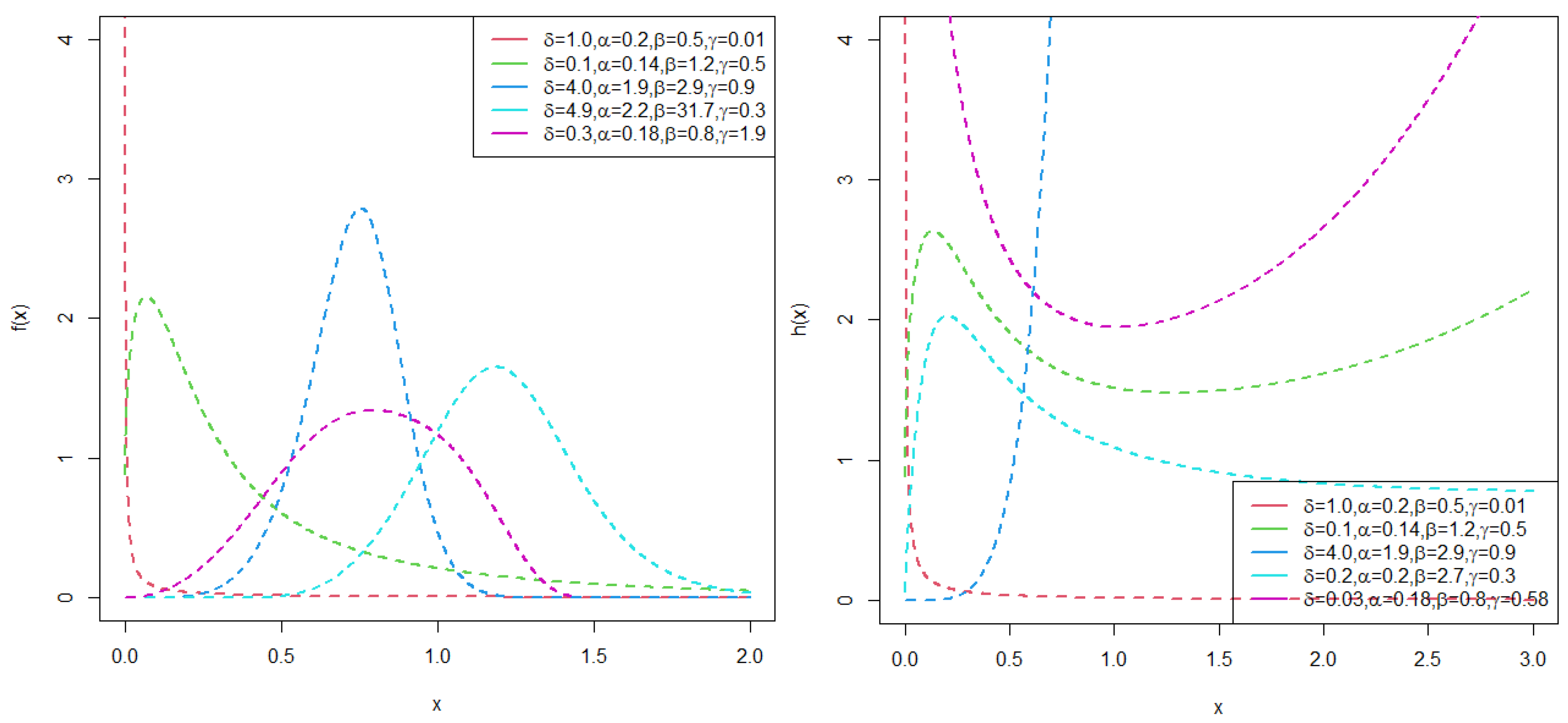
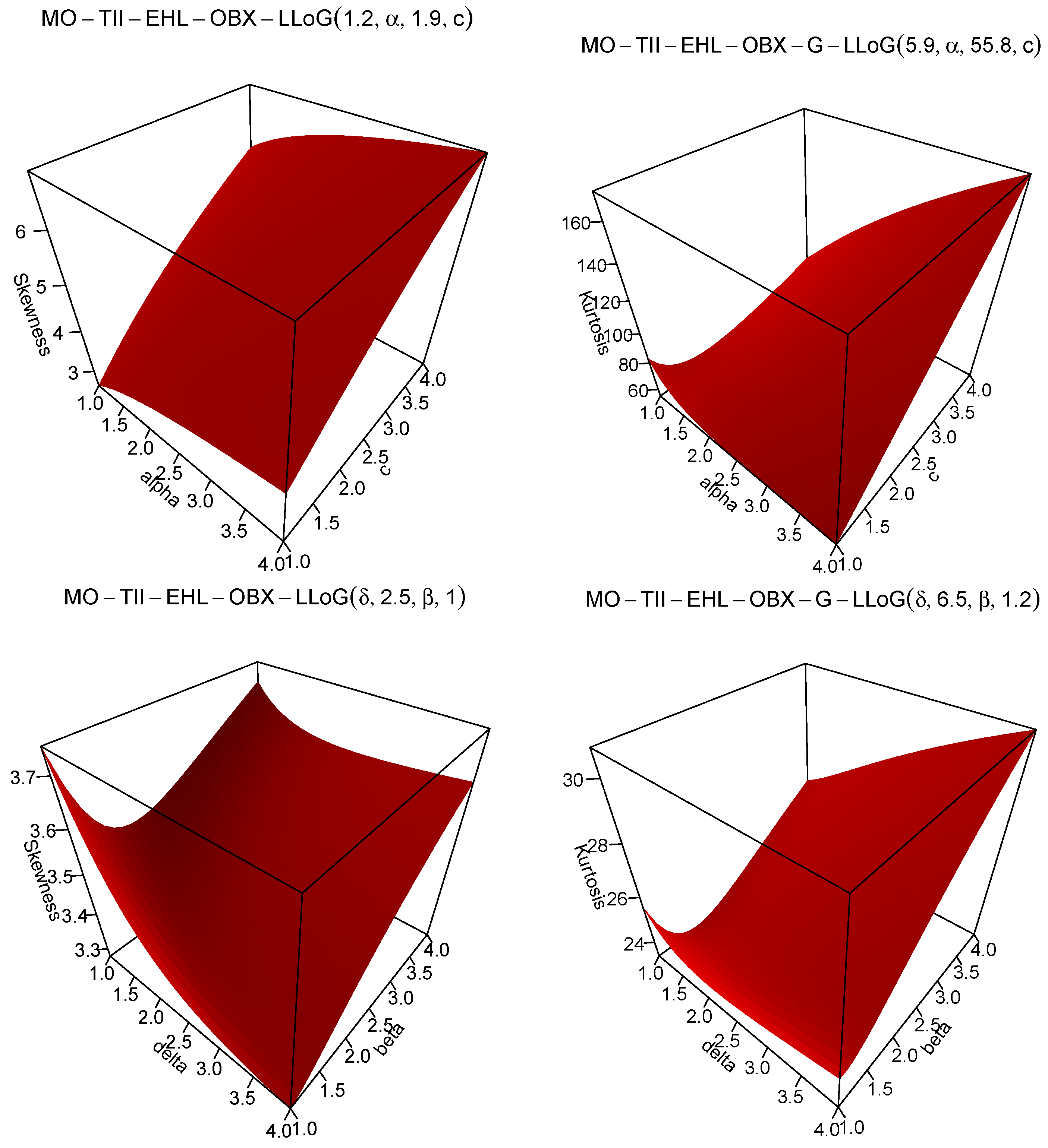
4.2. Marshall–Olkin–Type II Exponentiated Half-Logistic–Odd Burr X–Log-Logistic (MO-TIIEHL-OBX-LLoG) Distribution

Suppose we take the baseline distribution to be the log-logistic distribution with the cdf and pdf given by G ( x ; c ) = 1 ( 1 + x c ) 1 and g ( x ; c ) = c x c 1 ( 1 + x c ) 2 , respectively, for c , x > 0 . From Equations (7) and (8), we obtain the cdf and pdf of the MO-TIIEHL-OBX-LLoG distribution as
F ( x ; δ , α , β , c ) = 1 δ 1 1 exp 1 ( 1 + x c ) 1 ( 1 + x c ) 1 2 β 1 + 1 exp 1 ( 1 + x c ) 1 ( 1 + x c ) 1 2 β α 1 1 δ 1 1 exp 1 ( 1 + x c ) 1 ( 1 + x c ) 1 2 β 1 + 1 exp 1 ( 1 + x c ) 1 ( 1 + x c ) 1 2 β α ,
and
f ( x ; δ , α , β , c ) = 4 δ α β 1 ( 1 + x c ) 1 c x c 1 ( 1 + x c ) 2 ( 1 + x c ) 1 3 × exp 1 ( 1 + x c ) 1 ( 1 + x c ) 1 2 × 1 exp 1 ( 1 + x c ) 1 ( 1 + x c ) 1 2 β 1 × 1 1 exp 1 ( 1 + x c ) 1 ( 1 + x c ) 1 2 β α 1 × 1 + 1 exp 1 ( 1 + x c ) 1 ( 1 + x c ) 1 2 β ( α + 1 ) × 1 1 δ 1 1 exp 1 ( 1 + x c ) 1 ( 1 + x c ) 1 2 β 1 + 1 exp 1 ( 1 + x c ) 1 1 ( 1 + x c ) 1 2 β α 2 ,
respectively, for x , δ , α , β , and c > 0 .
Plots of the pdf and hrf of the MO-TIIEHL-OBX-LLoG distribution are given in Figure 3. The pdf of the MO-TIIEHL-OBX-LLoG distribution takes several shapes including reverse-J, right-skewed, and left-skewed, as well as almost symmetric, whereas the hrf displays bathtub, upside-down bathtub, upside-down bathtub followed by bathtub, decreasing, and increasing shapes.
Figure 4 presents the skewness and kurtosis plots for the MO-TIIEHL-OBX-LLoG distribution. The skewness and kurtosis increase with higher values of α and c, while they both exhibit a decreasing and then increasing trend with increasing values of δ and β .

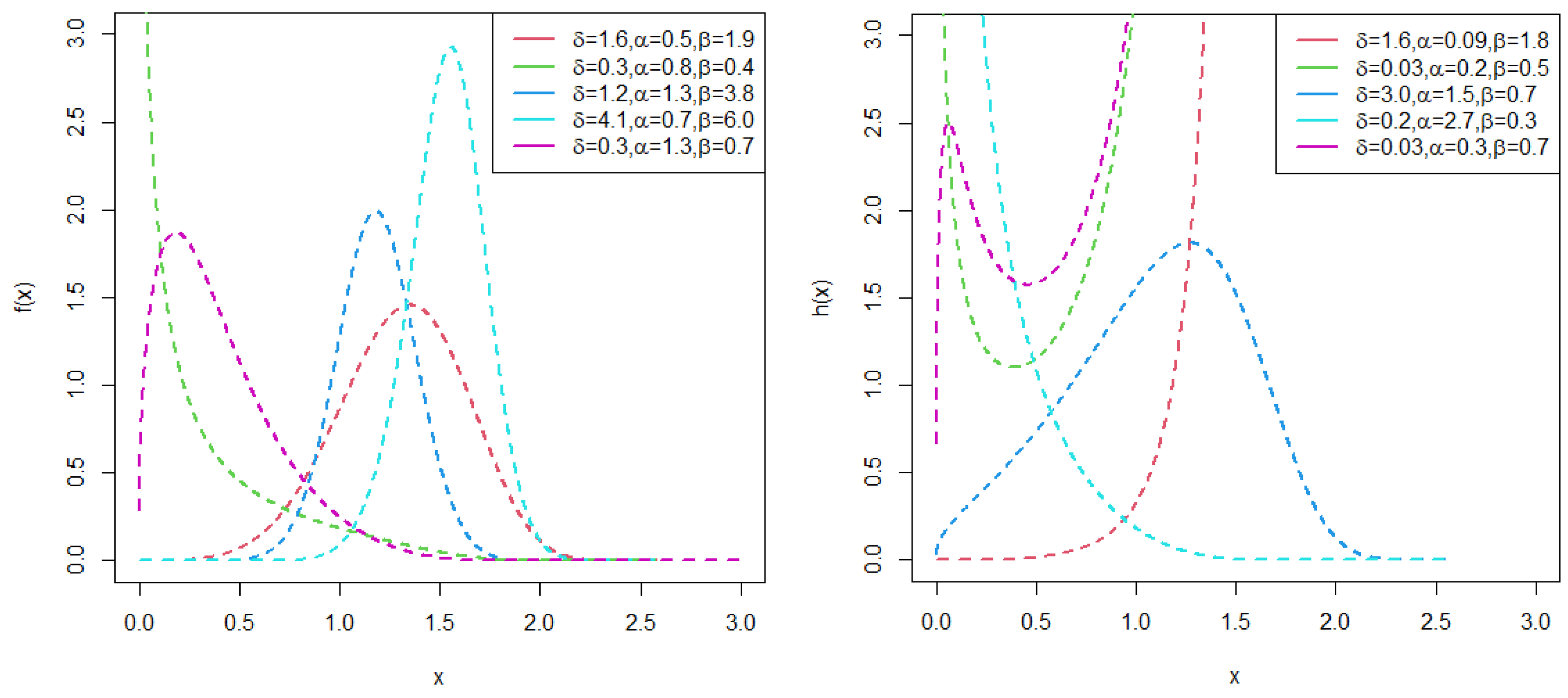
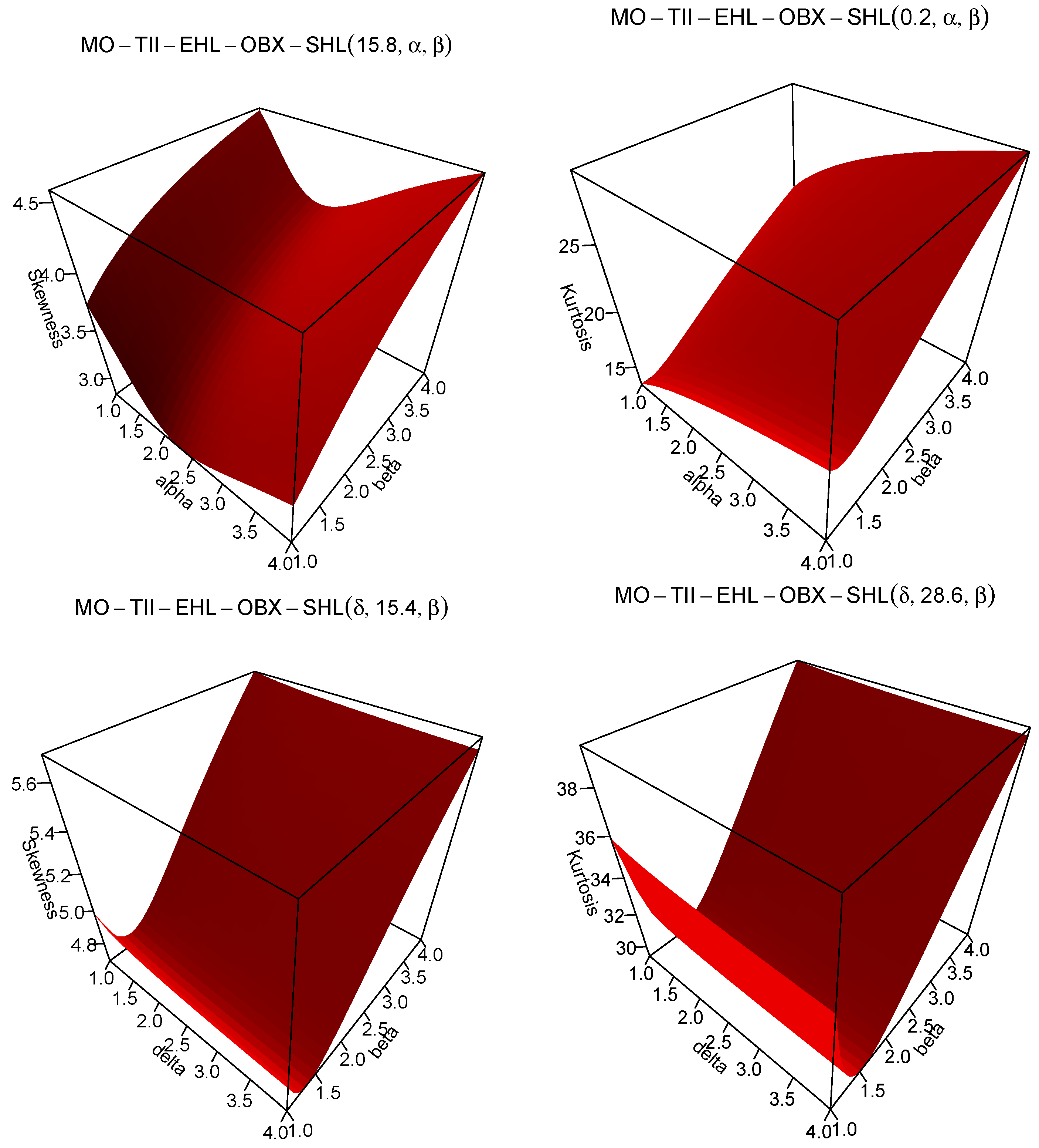
4.3. Marshall–Olkin–Type II Exponentiated Half-Logistic–Odd Burr X–Standard Half-Logistic (MO-TIIEHL-OBX-SHL) Distribution
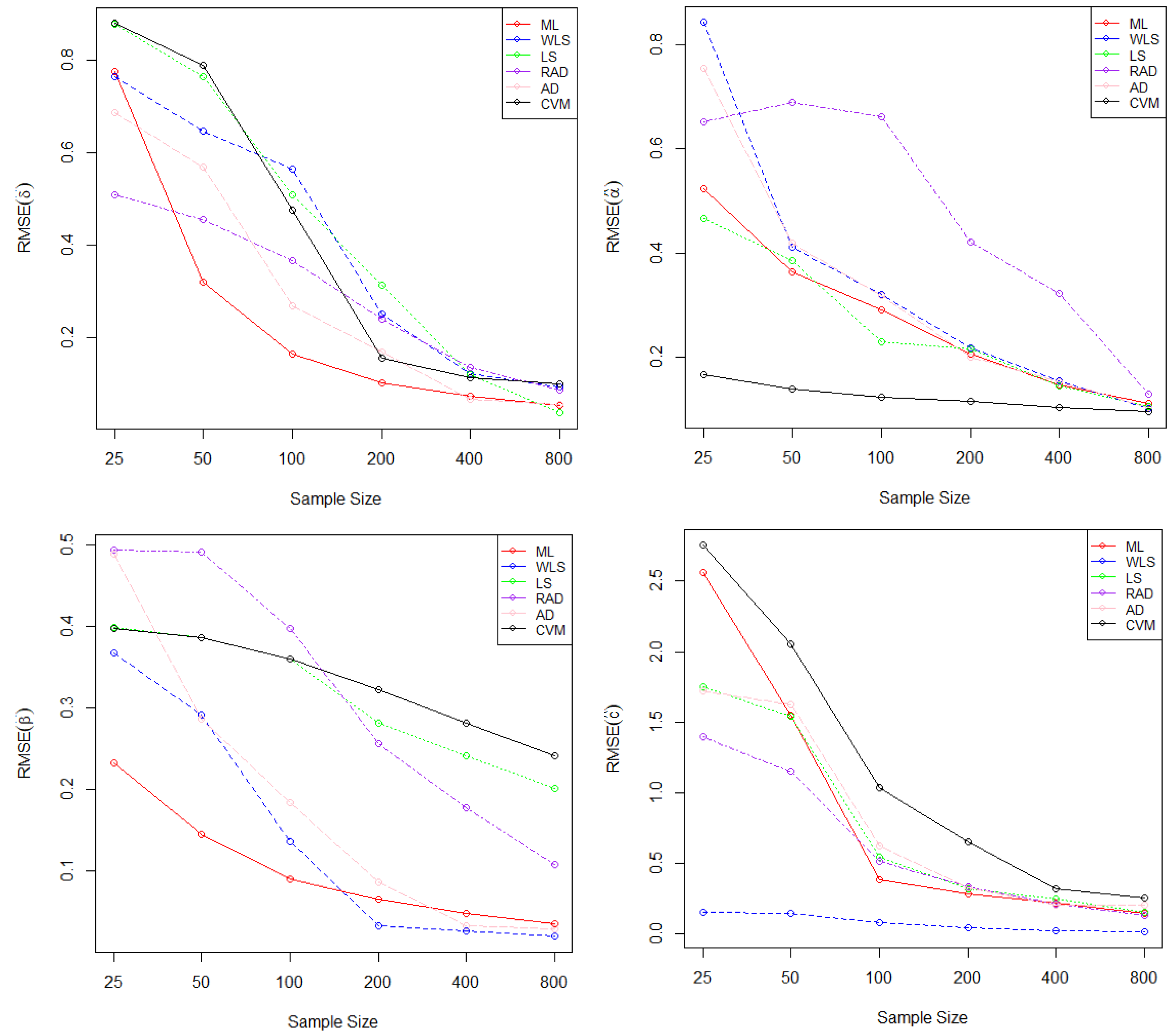
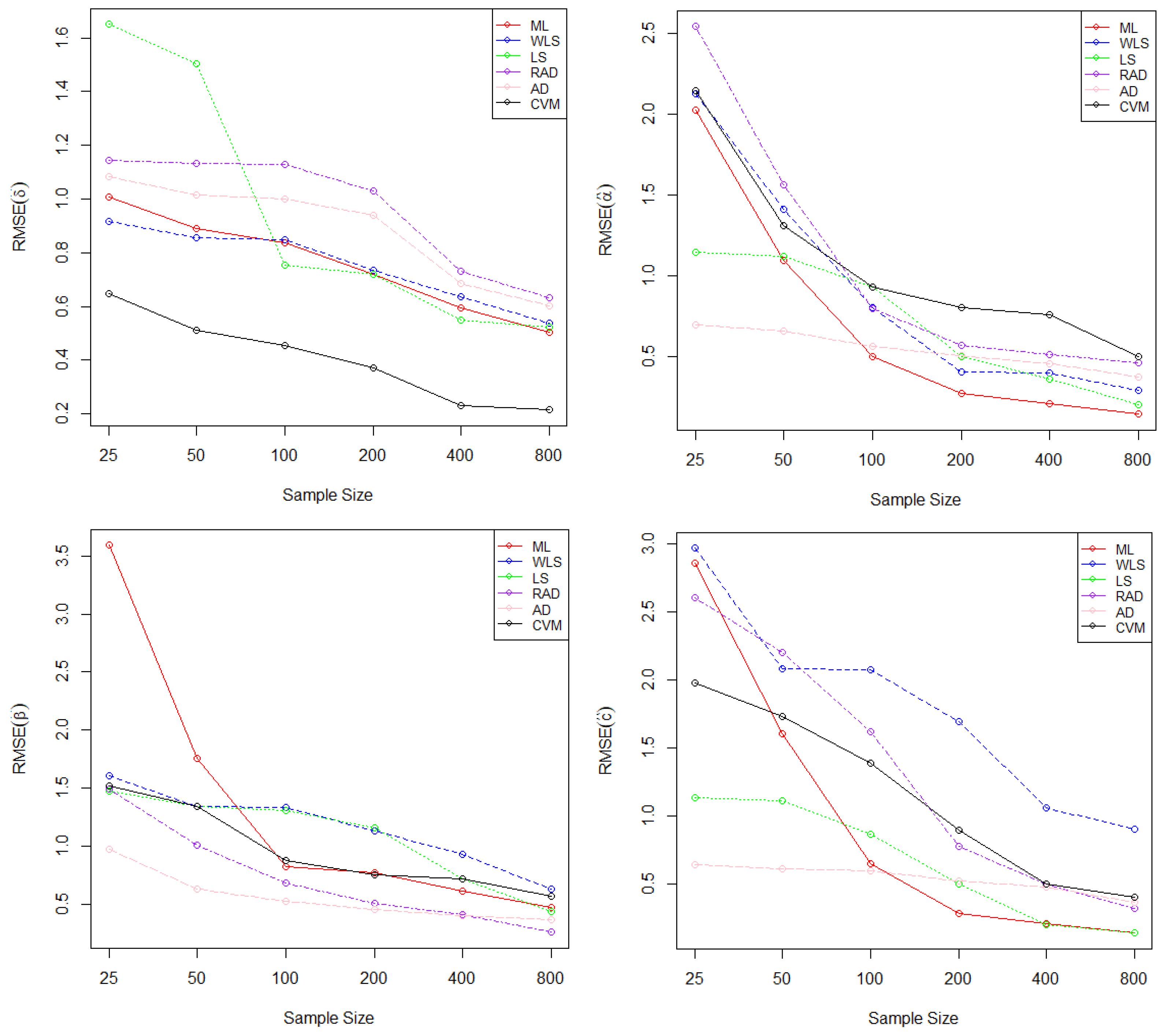
Suppose the baseline distribution is the standard half-logistic distribution, with the cdf and pdf given by G ( x ) = 1 e x 1 + e x and g ( x ) = 2 e x ( 1 + e x ) 2 , respectively, for x > 0 . From Equations (7) and (8), we obtain the cdf and pdf of the MO-TIIEHL-OBX-SHL distribution as
F ( x ; δ , α , β ) = 1 δ 1 1 exp 1 e x 2 e x 2 β 1 + 1 exp 1 e x 2 e x 2 β α 1 1 δ 1 1 exp 1 e x 2 e x 2 β 1 + 1 exp 1 e x 2 e x 2 β α ,
and
f ( x ; δ , α , β ) = 4 δ α β 2 e x 1 e x 1 + e x 3 1 1 e x 1 + e x 3 exp 1 e x 2 e x 2 × 1 exp 1 e x 2 e x 2 β 1 × 1 1 exp 1 e x 2 e x 2 β α 1 × 1 + 1 exp 1 e x 2 e x 2 β ( α + 1 ) × 1 1 δ 1 1 exp 1 e x 2 e x 2 β 1 + 1 exp 1 e x 2 e x 2 β α 2 ,
respectively, for x , δ , α , and β > 0 .
Figure 5 presents the plots of the pdf and hrf for the MO-TIIEHL-OBX-SHL distribution. The pdf of the MO-MO-TIIEHL-OBX-SHL distribution exhibits various shapes, including reverse-J, right-skewed, left-skewed, and nearly symmetric shapes. Meanwhile, the hrf demonstrates diverse patterns such as bathtub, inverted bathtub, an inverted bathtub followed by a bathtub, and an increasing trend.
Figure 6 presents the skewness and kurtosis plots for the MO-TIIEHL-OBX-SHL distribution. Both skewness and kurtosis increase with higher values of α and β . However, they exhibit a decreasing-then-increasing pattern as δ and β increase.

5. Simulation Study

The effectiveness of the parameter estimates for the MO-TIIEHL-OBX-LLoG distribution obtained through six estimation methods is examined by conducting various simulations for different sample sizes (n = 25, 50, 100, 200, 400, and 800) via the R package. The estimation methods include Maximum Likelihood Estimation (ML), Anderson–Darling (AD), Right-Tail Anderson–Darling (RAD), Ordinary Least Squares (OLS), Weighted Least Squares (WLS), and Cramér–von Mises (CVM). We simulate N = 3000 samples for the true parameter values given in Table 1 and Table 2. The tables list the average bias (Abias) and root mean square errors (RMSEs) of the model parameters as measures of the effectiveness and consistency of the parameter estimates. The Abias and RMSE for the estimated parameter, say η ^ , are given by
A b i a s ( η ^ ) = i = 1 N η ^ i N η , and R M S E ( η ^ ) = i = 1 N ( η ^ i η ) 2 N ,
respectively.
RMSE plots for different estimation methods are shown in Figure 7 and Figure 8. We note that the RMSE declines with an increase in sample size.
Table 3 presents the partial and overall rankings of different estimation methods for the MO-TIIEHL-OBX-LLoG distribution across various parameter values. The findings suggest that the MO-TIIEHL-OBX-LLoG distribution exhibits stability, as the Abias and RMSE occasionally decrease with increasing sample size across all estimation methods. Furthermore, Table the results highlight that the MLE method provides the most accurate estimates for the MO-TIIEHL-OBX-LLoG parameters, followed by the AD and LS methods, whereas the RAD method exhibits the weakest performance.

6. Risk Measures

This section explores key risk measures frequently utilized by financial and actuarial professionals to evaluate market risk exposure in an investment portfolio. These measures include Value at Risk (VaR), Tail Value at Risk (TVaR), Tail Variance (TV), and Tail Variance Premium (TVP).

6.1. Value at Risk

VaR is a widely used actuarial measure for evaluating financial market risk. It is typically expressed with a specified confidence level, such as ( 90 % , 95 % , or 99 % ). The VaR for the MO-TIIEHL-OBX-G family of distributions is defined as follows:
V a R θ = G 1 log 1 1 1 θ δ + ( 1 θ ) δ ¯ 1 α 1 + 1 θ δ + ( 1 θ ) δ ¯ 1 α 1 β 1 2 1 + log 1 1 1 θ δ + ( 1 θ ) δ ¯ 1 α 1 + 1 θ δ + ( 1 θ ) δ ¯ 1 α 1 β 1 2 ,
where θ ( 0 , 1 ) is a specified level of significance.

6.2. Tail Value at Risk

The TVaR represents the expected loss given that an event exceeding the predefined probability threshold has occurred. It provides a more comprehensive assessment of risk by considering extreme losses beyond the VaR level. The TVaR for the MO-TIIEHL-OBX-G family of distributions is defined as follows:
T V a R θ = E ( X X > x θ ) = 1 1 θ V a R θ x f ( x ) d x = 1 1 θ q = 0 V a R θ x ω q + 1 h q + 1 ( x ; Ξ ) d x ,
where ω q + 1 is given in Equation (11) and h q + 1 ( x ; Ξ ) = ( h + 1 ) G q ( x ; Ξ ) g ( x ; Ξ ) is the pdf of the exp-G distribution with the power parameter ( q + 1 ) .

6.3. Tail Variance

The TV measures the variability of losses beyond the VaR threshold, providing insight into the dispersion of extreme losses. The TV for the MO-TIIEHL-OBX-G family of distributions is defined as follows:
T V θ = E ( X 2 X > x θ ) ( T V a R θ ) 2 = 1 1 θ V a R θ x 2 f ( x ) d x ( T V a R θ ) 2 = 1 1 θ q = 0 ω q + 1 V a R θ x 2 h q + 1 ( x ; Ξ ) d x ( T V a R θ ) 2 .

6.4. Tail Variance Premium

The TVP is an important risk measure widely used in insurance analysis. It quantifies the additional premium required to account for the variability of extreme losses beyond the VaR. The TVP for the MO-TIIEHL-OBX-G family of distributions is defined as follows:
T V P θ = T V a R θ + λ ( T V θ ) ,
where 0 < λ < 1 . The TVP of the MO-TIIEHL-OBX-G family of distributions can be obtained by substituting Equations (16) and (17) into Equation (18).

6.5. Numerical Study for the Risk Measures
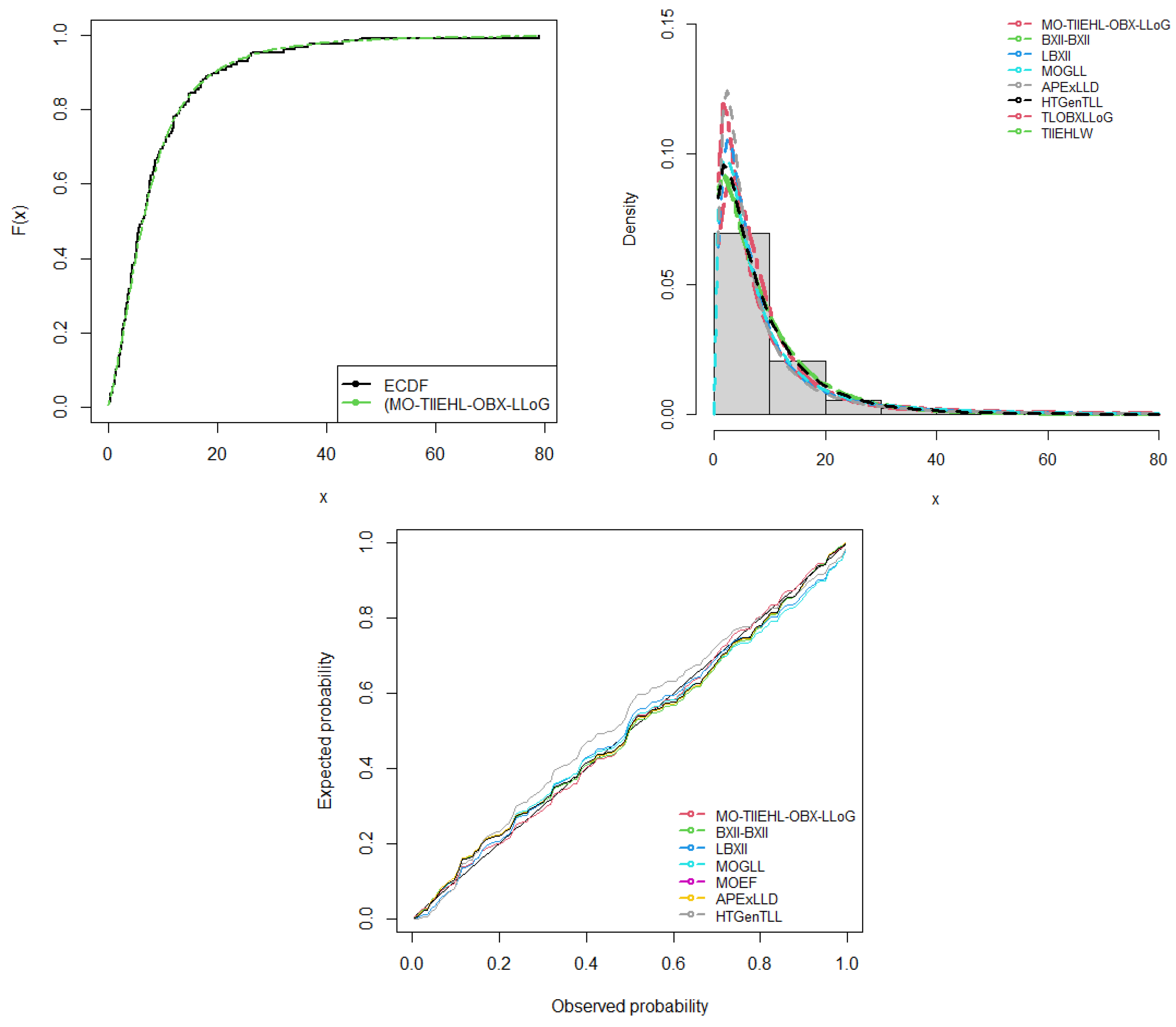
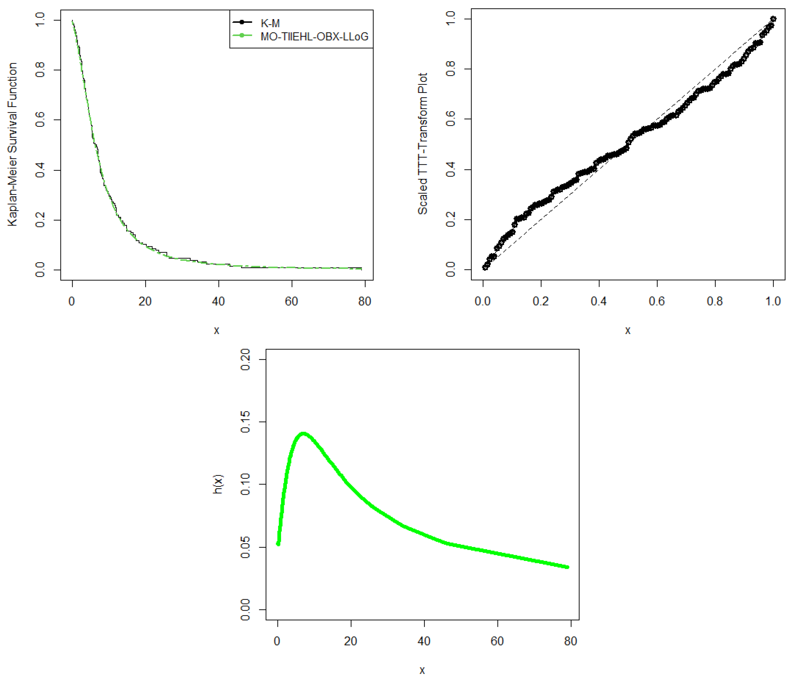
At this juncture, we assess the effectiveness of the MO-TIIEHL-OBX-LLoG distribution in modeling heavy-tailed data by conducting a numerical simulation of key risk measures. The results are then compared with those of its sub-models as well as equi-parameter models, specifically the Alpha Power Exponentiated Log-Logistic (APExLLD) distribution proposed by [21] and the Heavy-Tailed Generalized Topp–Leone Log-Logistic (HTGenTLL) distribution introduced by [22].
Table 4 presents the numerical results for the VaR, TVaR, TV, and TVP across the seven compared distributions. A distribution with higher values of these risk measures is considered to have a heavier tail. Based on the figures in Table 4, we conclude that the MO-TIIEHL-OBX-LLoG distribution exhibits a heavier tail than its sub-models and the non-nested equi-parameter APExLLD and HTGenTLL distributions. This makes it a suitable choice for modeling heavy-tailed data.

7. Applications

Examples are presented in this section to illustrate the usefulness of the MO-TIIEHL-OBX-LLoG distribution in applications using real data. Several goodness-of-fit statistics, including the -2log-likelihood (-2ln(L)), Akaike information criterion (AIC), and Bayesian information criterion (BIC) are employed to compare the MO-TIIEHL-OBX-LLoG distribution to other equi-parameter models. We also use the Cramér–von Mises ( W * ), Anderson–Darling ( A * ), and Kolmogorov–Smirnov (K-S) statistics as well as their associated p-values. In general, a better model fit is demonstrated by smaller values of goodness-of-fit statistics and the highest p-value for the K-S statistics. In addition, graphs including the Kaplan–Meier (K-M) survival plot, empirical cumulative distribution function (ECDF), total time on test (TTT) scaled plot, and probability plot are presented.
The MO-TIIEHL-OBX-LLoG distribution is compared to several distributions, including the type II exponentiated half-logistic Weibull (TIIEHLW) distribution by [5], the Topp–Leone–odd Burr X-log-logistic (TLOBXLLoG) distribution by [17], the Burr XII–Burr XII (BXII-BXII) distribution by [23], the logistic Burr XII (LBXII) distribution by [24], the Marshall–Olkin generalized log-logistic (MOGLL) distribution by [10], the Marshall–Olkin exponentiated Fréchet (MOEF) distribution by [25], the Alpha power exponentiated log-logistic (APExLLD) distribution by [21], and the heavy-tailed generalized Topp–Leone log-logistic (HTGenTLL) distribution by [22]. The pdf’s of these distributions are given in Appendix A.

7.1. Remission Time of Cancer Data

The dataset represents the remission times of 128 cancer patients. It was utilized in [26].
Table 5 presents the maximum likelihood estimates (MLEs), standard errors (SEs) (in parentheses), and goodness-of-fit statistics for the remission time data. Based on the values in Table 5, we conclude that the MO-TIIEHL-OBX-LLoG distribution provides a better fit compared to the other equi-parameter models, since it has the lowest values of the goodness-of-fit statistics 2 log ( L ) , A I C ,   C A I C ,   B I C , W * , A * , and K-S. The MO-TIIEHL-OBX-LLoG distribution’s p-value of the K S statistic is also the largest as compared to the other fitted distributions. Figure 9 and Figure 10 corroborate the results in Table 5.

7.2. Carbon Fiber Data

The dataset represents the breaking stress of carbon fibers with a length of 50 mm (GPa). It was recently utilized by [27] and is provided in Appendix A.
Table 6 presents the maximum likelihood estimates (MLEs), standard errors (SEs) (in parentheses), and goodness-of-fit statistics for the carbon fiber data. Based on the values in Table 6, we conclude that the MO-TIIEHL-OBX-LLoG distribution provides a better fit compared to the other equi-parameter models, since it has the lowest values of the goodness-of-fit statistics 2 log ( L ) , A I C ,   C A I C ,   B I C , W * , A * , and K-S. The MO-TIIEHL-OBX-LLoG distribution’s p-value of the K S statistic is also the largest as compared to the other fitted distributions. Figure 11 and Figure 12 corroborate the results in Table 6.

7.3. Height Data

The dataset consists of height measurements (in cm) recorded for 100 Australian female athletes. It was previously utilized by [28], and the complete observations are provided in Appendix A.
Table 7 presents the maximum likelihood estimates (MLEs), standard errors (SEs) (in parentheses), and goodness-of-fit statistics for the height data. Based on the values in Table 7, we conclude that the MO-TIIEHL-OBX-LLoG distribution provide a better fit compared to the other equi-parameter models, since it has the lowest values of 2 log ( L ) , A I C ,   C A I C ,   B I C , W * , A * , and K-S. The MO-TIIEHL-OBX-LLoG distribution’s p-value of the K S statistic is also the largest as compared to the other fitted distributions. Figure 13 and Figure 14 corroborate the results in Table 7.

8. Conclusions

A new generalized family of distributions called the Marshall–Olkin–type II exponentiated half-logistic–odd Burr X-G (MO-TIIEHL-OBX-G) family of distributions was developed and presented. The density of the new family of distributions can be expressed as an infinite linear combination of exponentiated-G densities. The hazard rate functions of the new family of distributions are quite flexible, with monotone and non-monotone shapes. We also obtain expressions for the moments, distribution of order statistics, probability-weighted moments, and Rényi entropy. The performance of the special case of the MO-TIIEHL-OBX-G distribution was evaluated by conducting various simulations across different sample sizes to assess the efficiency of different estimation methods. Risk measures for this distribution were also presented, and the results revealed that the Marshall–Olkin–type II exponentiated half-logistic–odd Burr X–log-logistic (MO-TIIEHL-OBX-LLoG) distribution is heavy-tailed. Finally, the special case of the MO-TIIEHL-OBX-LLoG distribution was fitted to three real datasets to illustrate the importance and applicability of the proposed family of distributions.
Future research on the MO-TIIEHL-OBX-G family of distributions could focus on extending its application to higher-dimensional data, allowing for multivariate modeling. Additionally, the proposed distribution could be applied to censored data scenarios using real-world datasets, including type-II progressive hybrid censored data, type-II double-censored data, and step-stress-accelerated data. Another promising direction is the incorporation of Bayesian estimation techniques, which could provide a more robust framework for parameter estimation, especially in the presence of small sample sizes and prior information.

Author Contributions

Conceptualization, B.O.; methodology, B.O. and T.M.; software, T.M., B.O. and G.L.; formal analysis, B.O., G.L. and T.M.; writing—review and editing, B.O., T.M. and G.L. All authors have read and agreed to the published version of the manuscript.

Funding

This research received no external funding.

Institutional Review Board Statement

Not applicable.

Informed Consent Statement

Not applicable.

Data Availability Statement

Data is contained within the article.

Conflicts of Interest

The authors declare no conflicts of interest.

Appendix A

Competing Models

The pdfs of the competing models are as follows:
f T I I E H L W ( x ; a , λ , δ , γ ) = 2 a λ δ γ x γ 1 exp δ x γ β [ 1 [ 1 exp δ x γ ] γ ] a 1 [ 1 + [ 1 exp δ x γ ] γ ] a + 1
for a , λ , δ , γ > 0 , and x > 0 ;
f T L O B X L L o G ( x ; α , θ , β ) = 4 α θ β x β 1 ( 1 + x β ) ( 1 ( 1 + x β ) 1 ) exp [ x 2 β ] { 1 exp [ x 2 β ] } θ 1 × 1 { 1 exp [ x 2 β ] } θ 1 1 { 1 exp [ x 2 β ] } θ 2 α 1
for α , θ , β > 0 , and x > 0 ;
f M O E F ( x ; α , λ , δ , β ) = β α λ δ λ 1 exp δ x λ α 1 x ( 1 + λ ) exp δ x λ 1 1 β 1 exp δ x λ α 2 ,
for α , λ , δ , β > 0 ;
f L B X I I ( x ; λ , d , c , s ) = λ c d λ s c x c 1 1 + x s c log 1 + x s c ( λ + 1 ) × 1 + d log 1 + x s c λ 2 ,
for λ , d , c , s > 0 ;
f A P E X L L D ( x ; α , a , b , c ) = a c l o g ( α ) b ( α 1 ) x b a 1 x b a + 1 c 1 α ( x b a + 1 ) c ,
for α , a , b , c > 0 , and x > 0 ;
f B X I I B X I I ( x ; a , b , α , β ) = a b α β x a 1 x a + 1 b 1 x a + 1 b + 1 α 1 x a + 1 b 1 α + 1 β + 1 ,
for a , b , α , β > 0 , and x > 0 ;
f M O G L L ( x ; δ , a , α , β ) = δ a β α β x β 1 1 + x a β a 1 1 1 δ 1 + x a β a 2 ,
for δ , a , α , β > 0 , and x > 0 ; and
f H T G e n T L L ( x ; b , θ , c , β ) = 2 b β θ 2 c x c 1 1 + x c 2 1 1 + x c 2 b 1 1 + x c 1 × 1 1 1 + x c 2 b β θ 1 × 1 1 θ 1 1 1 1 + x c 2 b β ( θ + 1 ) ,
for b , θ , c , β > 0 , and x > 0 .

Application Data Sets

Remission Time Data
0.08, 4.98, 25.74, 3.7, 10.06, 2.69, 7.62, 1.26, 7.87, 4.4, 2.02, 21.73, 2.09, 6.97, 0.5, 5.17, 14.77, 4.18, 10.75, 2.83, 11.64, 5.85, 3.31, 2.07, 3.48, 9.02, 2.46, 7.28, 32.15, 5.34, 16.62, 4.33, 17.36, 8.26, 4.51, 3.36, 4.87, 13.29, 3.64, 9.74, 2.64, 7.59, 43.01, 5.49, 1.4, 11.98, 6.54, 6.93, 6.94, 0.4, 5.09, 14.76, 3.88, 10.66, 1.19, 7.66, 3.02, 19.13, 8.53, 8.65, 8.66, 2.26, 7.26, 26.31, 5.32, 15.96, 2.75, 11.25, 4.34, 1.76, 12.03, 12.63, 13.11, 3.57, 9.47, 0.81, 7.39, 36.66, 4.26, 17.14, 5.71, 3.25, 20.28, 22.69, 23.63, 5.06, 14.24, 2.62, 10.34, 1.05, 5.41, 79.05, 7.93, 4.5, 2.02, 0.2, 7.09, 25.82, 3.82, 14.83, 2.69, 7.63, 1.35, 11.79, 6.25, 3.36, 2.23, 9.22, 0.51, 5.32, 34.26, 4.23, 17.12, 2.87, 18.1, 8.37, 6.76, 3.52, 13.8, 2.54, 7.32, 0.9, 5.41, 46.12, 5.62, 1.46, 12.02, 12.07.
Carbon Fiber Data
0.39, 0.85, 1.08, 1.25, 1.47, 1.57, 1.61, 1.61, 1.69, 1.80, 1.84, 1.87, 1.89, 2.03, 2.03, 2.05, 2.12, 2.35, 2.41, 2.43, 2.48, 2.50, 2.53, 2.55, 2.55, 2.56, 2.59, 2.67, 2.73, 2.74, 2.79, 2.81, 2.82, 2.85, 2.87, 2.88, 2.93, 2.95, 2.96, 2.97, 3.09, 3.11, 3.11, 3.15, 3.15, 3.19, 3.22, 3.22, 3.27, 3.28, 3.31, 3.31, 3.33, 3.39, 3.39, 3.56, 3.60, 3.65, 3.68, 3.70, 3.75, 4.20, 4.38, 4.42, 4.70, 4.90.
Height Data
148.9, 149.0, 156.0, 156.9, 157.9, 158.9, 162.0, 162.0, 162.5, 163.0, 163.9, 165.0, 166.1, 166.7, 167.3, 167.9, 168.0, 168.6, 169.1, 169.8, 169.9, 170.0, 170.0, 170.3, 170.8, 171.1, 171.4, 171.4, 171.6, 171.7, 172.0, 172.2, 172.3, 172.5, 172.6, 172.7, 173.0, 173.3, 173.3, 173.5, 173.6, 173.7, 173.8, 174.0, 174.0, 174.0, 174.1, 174.1, 174.4, 175.0, 175.0, 175.0, 175.3, 175.6, 176.0, 176.0, 176.0, 176.0, 176.8, 177.0, 177.3, 177.3, 177.5, 177.5, 177.8, 177.9, 178.0, 178.2, 178.7, 178.9, 179.3, 179.5, 179.6, 179.6, 179.7, 179.7, 179.8, 179.9, 180.2, 180.2, 180.5, 180.5, 180.9, 181.0, 181.3, 182.1, 182.7, 183.0, 183.3, 183.3, 184.6, 184.7, 185.0, 185.2, 186.2, 186.3, 188.7, 189.7, 193.4, 195.9.
Codes Parameter Estimation
  • x<-c(0.08, 4.98, 25.74, 3.7, 10.06, 2.69, 7.62, 1.26, 7.87, 4.4,
  • 2.02, 21.73, 2.09, 6.97, 0.5, 5.17, 14.77, 4.18, 10.75, 2.83,
  • 11.64, 5.85, 3.31, 2.07, 3.48, 9.02, 2.46, 7.28, 32.15, 5.34,
  • 16.62, 4.33, 17.36, 8.26, 4.51, 3.36, 4.87, 13.29, 3.64, 9.74,
  • 2.64, 7.59, 43.01, 5.49, 1.4, 11.98, 6.54, 6.93, 6.94, 0.4, 5.09,
  • 14.76, 3.88, 10.66, 1.19, 7.66, 3.02, 19.13, 8.53, 8.65, 8.66,
  • 2.26 ,7.26 ,26.31, 5.32, 15.96, 2.75, 11.25, 4.34, 1.76, 12.03,
  • 12.63, 13.11, 3.57, 9.47, 0.81, 7.39, 36.66, 4.26, 17.14, 5.71,
  • 3.25, 20.28, 22.69, 23.63, 5.06, 14.24, 2.62, 10.34, 1.05, 5.41,
  • 79.05, 7.93, 4.5, 2.02, 0.2 ,7.09, 25.82, 3.82, 14.83, 2.69, 7.63,
  • 1.35, 11.79, 6.25, 3.36, 2.23, 9.22, 0.51, 5.32, 34.26 ,4.23, 17.12,
  • 2.87, 18.1, 8.37, 6.76 ,3.52, 13.8, 2.54, 7.32 ,0.9 ,5.41, 46.12,
  • 5.62, 1.46, 12.02 ,12.07
  • )
  • .
  • .
  • ## MO-TIIEHL-OBX-LLoG
  • fMOTIIEHLOBXLLoG<-function(delta  ,alpha ,beta ,c)
  • {
  •   −sum(log(4∗delta∗alpha∗beta∗(c∗((1+x^c)^(−2))∗(x^(c−1)))∗
  •   ((1−(1+x^c)^(−1))/((1+x^c)^(−1))^3)∗
  •   (exp(−((1−(1+x^c)^(−1))/((1+x^c)^(−1)))^2))∗
  •   ((1−exp(−((1−(1+x^c)^(−1))/((1+x^c)^(−1)))^2))^(beta−1))
  •   ∗((1+(1−exp(−((1−(1+x^c)^(−1))/((1+x^c)
  •   ^(−1)))^2))^beta)^(−(alpha+1)))∗((1−(1−exp(−((1−(1+x^c)^(−1))
  •   /((1+x^c)^(−1)))^2))^beta)^(alpha−1))
  •   ∗((1−(1−delta)∗((1−(1−exp(−((1−(1+x^c)
  •   ^(−1))/((1+x^c)^(−1)))^2))^beta)
  •   /(1+(1−exp(−((1−(1+x^c)^(−1))/((1+x^c)^(−1)))^2))^beta))
  •   ^alpha))^(−2)
  • ))
  • }
  • MOTIIEHLOBXLLoG.result<-mle2(fMOTIIEHLOBXLLoG, hessian = NULL,
  • start=list(delta=939.8992, alpha=91.96, beta=11.099, c=.088),
  • optimizer="nlminb" ,lower=0)
  • summary(MOTIIEHLOBXLLoG.result)

Goodness-of-Fit Test

  • library(AdequacyModel)
  • .
  • data=c(0.08, 4.98, 25.74, 3.7, 10.06, 2.69, 7.62, 1.26, 7.87, 4.4,
  • 2.02, 21.73, 2.09, 6.97, 0.5, 5.17, 14.77, 4.18, 10.75, 2.83,
  • 11.64, 5.85, 3.31, 2.07, 3.48, 9.02, 2.46, 7.28, 32.15, 5.34,
  • 16.62, 4.33, 17.36, 8.26, 4.51, 3.36, 4.87, 13.29, 3.64, 9.74,
  • 2.64, 7.59, 43.01, 5.49, 1.4, 11.98, 6.54, 6.93, 6.94, 0.4, 5.09,
  • 14.76, 3.88, 10.66, 1.19, 7.66, 3.02, 19.13, 8.53, 8.65, 8.66,
  • 2.26 ,7.26 ,26.31, 5.32, 15.96, 2.75, 11.25, 4.34, 1.76, 12.03,
  • 12.63, 13.11, 3.57, 9.47, 0.81, 7.39, 36.66, 4.26, 17.14, 5.71,
  • 3.25, 20.28, 22.69, 23.63, 5.06, 14.24, 2.62, 10.34, 1.05, 5.41,
  • 79.05, 7.93, 4.5, 2.02, 0.2 ,7.09, 25.82, 3.82, 14.83, 2.69, 7.63,
  • 1.35, 11.79, 6.25, 3.36, 2.23, 9.22, 0.51, 5.32, 34.26 ,4.23, 17.12,
  • 2.87, 18.1, 8.37, 6.76 ,3.52, 13.8, 2.54, 7.32 ,0.9 ,5.41, 46.12,
  • 5.62, 1.46, 12.02 ,12.07
  • )
  • .
  • .
  • MOTIIEHLOBXLLoG_pdf<-function(par,x){
  •  delta=par[1]
  •    alpha=par[2]
  •   beta=par[3]
  •  c=par[4]
  • 4∗delta∗alpha∗beta∗(c∗((1+x^c)^(−2))∗(x^(c−1)))∗((1−(1+x^c)^(−1))
  • /((1+x^c)^(−1))^3)∗(exp(−((1−(1+x^c)^(−1))/((1+x^c)^(−1)))^2))
  • ∗((1−exp(−((1−(1+x^c)^(−1))/((1+x^c)^(−1)))^2))^(beta−1))
  • ∗((1+(1−exp(−((1−(1+x^c)^(−1))/((1+x^c)^(−1)))^2))^beta)
  • ^(−(alpha+1)))∗((1−(1−exp(−((1−(1+x^c)^(−1))/((1+x^c)^(−1)))^2))
  • ^beta)^(alpha−1))∗((1−(1−delta)∗((1−(1−exp(−((1−(1+x^c)^(−1))
  • /((1+x^c)^(−1)))^2))^beta)/(1+(1−exp(−((1−(1+x^c)^(−1))
  • /((1+x^c)^(−1)))^2))^beta))^alpha))^(−2)
  • }
  • MOTIIEHLOBXLLoG_cdf<-function(par,x){
  •    delta=par[1]
  •       alpha=par[2]
  •      beta=par[3]
  •    c=par[4]
  • .
  • 1-(delta∗((1-(1-exp(-((1-(1+x^c)^(-1))/((1+x^c)^(-1)))^2))^beta)
  • /(1+(1-exp(-((1-(1+x^c)^(-1))/((1+x^c)^(-1)))^2))^beta)
  • )^alpha)/(1-(1-delta)∗((1-(1-exp(-((1-(1+x^c)^(-1))
  • /((1+x^c)^(-1)))^2))^beta)/(1+(1-exp(-((1-(1+x^c)^(-1))
  • /((1+x^c)^(-1)))^2))^beta)
  • )^alpha)}
  • goodness.fit(pdf=MOTIIEHLOBXLLoG_pdf, cdf=MOTIIEHLOBXLLoG_cdf,
  • mle=c( 9.6978e+02   , 1.1338e+01 ,   3.7292e+00  ,    6.5701e-02 ),
  • data = data,method = "BFGS",
  •                domain = c(0,Inf), lim_inf = c(0,0,0,0),
  •                lim_sup = c(10000000000000000,100000000000000,
  •                10000000000000000,10000000000000000))

References

  1. Marshall, A.W.; Olkin, I. A new method for adding a parameter to a family of distributions with application to the exponential and Weibull families. Biometrika 1997, 83, 641–652. [Google Scholar] [CrossRef]
  2. Yousof, H.M.; Afify, A.Z.; Hamedani, G.; Aryal, G.R. The Burr X generator of distributions for lifetime data. J. Stat. Theory Appl. 2017, 16, 288–305. [Google Scholar] [CrossRef]
  3. Al-Shomrani, A.; Arif, O.; Shawku, K.; Harif, S.; Shahbaz, M.Q. Topp-Leone family of distributions: Some properties and applications. Pak. J. Stat. Oper. Res. 2016, 12, 443–451. [Google Scholar] [CrossRef]
  4. Hassan, A.S.; Elgarhy, M.; Shakil, M. Type II half-logistic family of distributions with applications. Pak. J. Stat. Oper. Res. 2017, 13, 245–264. [Google Scholar]
  5. Al-Mofleh, H.; Elgarhy, M.; Afify, A.Z.; Zannon, M.S. Type II exponentiated half-logistic generated family of distributions with applications. Electron. J. Appl. Stat. Anal. 2020, 13, 536–561. [Google Scholar]
  6. Zografos, K.; Balakrishnan, N. On families of Beta and generalized gamma-generated distributions and associated inference. Stat. Methodol. 2009, 6, 344–362. [Google Scholar] [CrossRef]
  7. Ristić, M.M.; Balakrishnan, N. The gamma-exponentiated exponential distribution. J. Stat. Comput. Simul. 2012, 82, 1191–1206. [Google Scholar] [CrossRef]
  8. Khaleel, M.A.; Oguntunde, P.E.; Al Abbasi, J.N.; Ibrahim, N.A.; Abujarad, M.H. The Marshall–Olkin Topp–Leone-G family of distributions with applications. Sci. Afr. 2020, 8, e00470. [Google Scholar]
  9. Al-Saiari, A.Y.; Baharith, L.A.; Mousa, S.A. Marshall-Olkin extended Burr type XII distribution. Int. J. Stat. Probab. 2014, 3, 78–84. [Google Scholar] [CrossRef]
  10. Yousof, H.M.; Afify, A.Z.; Nadarajah, S.; Hamedani, G.; Aryal, G.R. The Marshall-Olkin gerenalized-G family of distributions with applications. Statistica 2018, 78, 273–295. [Google Scholar]
  11. Krishna, E.; Jose, K.K.; Alice, T.; Ristić, M.M. The Marshall-Olkin Fréchet distribution. Commun. Stat.-Theory Methods 2013, 42, 4091–4107. [Google Scholar] [CrossRef]
  12. Ristić, M.M.; Kundu, D. Marshall-Olkin generalized exponential distribution. Metron 2015, 73, 317–333. [Google Scholar] [CrossRef]
  13. Almetwall, E.M.; Sabry, M.A.H.; Alharbi, R.; Alnagar, D.; Mubarak, S.A.M.; Hafez, E.H. Marshall-Olkin Alpha power Weibull distribution: Different methods of estimation based on type-I and type-II censoring. Complexity 2021, 1, 5533799. [Google Scholar] [CrossRef]
  14. Basheer, A.M. Marshall-Olkin alpha power inverse exponential distribution: Properties and aplications. Ann. Data Sci. 2022, 9, 301–313. [Google Scholar] [CrossRef]
  15. Mansoor, M.; Tahir, M.H.; Cordeiro, G.M.; Provost, S.B.; Alzaatreh, A. The Marshall-Olkin logistic exponential distribution. Commun. Stat.-Theory Methods 2019, 48, 220–234. [Google Scholar] [CrossRef]
  16. Dingalo, N.; Oluyede, B.; Chipepa, F. The type II exponentiated half logistic-odd Burr X-G power series class of distributions with applications. Heliyon 2023, 9, e22402. [Google Scholar] [CrossRef]
  17. Oluyede, B.; Tlhaloganyang, B.P.; Sengweni, W. The Topp-Leone odd Burr X-G family of distributions: Properties and applications. Stat. Optim. Inf. Comput. 2024, 12, 109–132. [Google Scholar] [CrossRef]
  18. Raghav, Y.S.; Ahmadini, A.A.H.; Mahnashi, A.M.; Rather, K.U.I. Enhancing estimation efficiency with proposed estimator: A comparative analysis of Poisson regression-based mean estimators. Kuwait J. Sci. 2025, 52, 100282. [Google Scholar] [CrossRef]
  19. Mishra, R.; Singh, R.; Raghav, Y.S. On combining ratio and product type estimators for estimation of finite population mean in adaptive cluster sampling design. Braz. J. Biom. 2024, 42, 412–420. [Google Scholar] [CrossRef]
  20. Rényi, A. On measures of information and entropy. In Proceedings of the 4th Berkeley Symposium on Mathematics, Statistics and Probability, Berkeley, CA, USA, 20 June–30 July 1960; Volume 1, pp. 547–561. [Google Scholar]
  21. Mead, M.E.; Cordeiro, G.M.; Afify, A.Z.; Al-Mofleh, H. The Alpha power transformation family: Properties and applications. Pak. J. Stat. Oper. Res. 2019, 15, 525–545. [Google Scholar] [CrossRef]
  22. Moakofi, T.; Oluyede, B.; Tlhaloganyang, B.; Puoetsile, A. A new family of heavy-tailed generalized Topp-Leone-G distributions with application. Pak. J. Stat. Oper. Res. 2024, 20, 233–260. [Google Scholar] [CrossRef]
  23. Gad, A.M.; Hamedani, G.G.; Salehabadi, S.M.; Yousof, H.M. The Burr XII-Burr XII distribution: Mathematical properties and characterizations. Pak. J. Stat. 2019, 35, 229–248. [Google Scholar]
  24. Guerra, R.; Peña-Ramírez, F.A.; Cordeiro, G.M. The logistic Burr XII distribution: Properties and applications to income data. Stats 2023, 6, 1260–1279. [Google Scholar] [CrossRef]
  25. Niyoyunguruza, A.; Odongo, L.; Nyarige, E.; Habaneza, A.; Muse, A. Marshall-Olkin exponentiated Fréchet distribution. J. Data Anal. Inf. Process. 2023, 11, 262–292. [Google Scholar]
  26. Lee, E.T.; Wang, J. Statistical Methods For Survival Data Analysis; John Wiley and Sons: Hoboken, NJ, USA, 2003; Volume 476. [Google Scholar]
  27. Telee, L.B.S.; Kumar, V. Some properties and applications of half-Cauchy exponential extension distribution. Int. J. Stat. Appl. Math. 2022, 7, 91–101. [Google Scholar] [CrossRef]
  28. Mustafa, A.; Khan, M.I. Length biased extended Rayleigh distribution and its applications. J. Mod. Appl. Stat. Methods 2023, 22. [Google Scholar]
Figure 1. Plots of the pdf and hrf for the MO-TIIEHL-OBX-W distribution.
Stats 08 00026 g001
Figure 2. Three-dimensional plots of skewness and kurtosis for the MO-TIIEHL-OBX-W distribution.
Stats 08 00026 g002
Figure 3. Plots of the pdf and hrf for the MO-TIIEHL-OBX-LLoG distribution.
Stats 08 00026 g003
Figure 4. Three-dimensional plots of skewness and kurtosis for the MO-TIIEHL-OBX-LLoG distribution.
Stats 08 00026 g004
Figure 5. Plots of the pdf and hrf for the MO-TIIEHL-OBX-SHL distribution.
Stats 08 00026 g005
Figure 6. Three-dimensional plots of skewness and kurtosis for the MO-TIIEHL-OBX-SHL distribution.
Stats 08 00026 g006
Figure 7. RMSE plots.
Stats 08 00026 g007
Figure 8. RMSE plots.
Stats 08 00026 g008
Figure 9. ECDF, fitted density, and probability plots for remission time data.
Stats 08 00026 g009
Figure 10. Kaplan–Meier survival plot, TTT plot, and hazard rate function plot for remission time data.
Stats 08 00026 g010
Figure 11. ECDF, fitted density, and probability plots for carbon fiber data.
Stats 08 00026 g011
Figure 12. Kaplan–Meier survival plot, TTT plot, and hazard rate function plot for carbon fiber data.
Stats 08 00026 g012
Figure 13. ECDF, fitted density, and probability plots for height data.
Stats 08 00026 g013
Figure 14. Kaplan–Meier survival plot, TTT plot, and hrf plot for height data.
Stats 08 00026 g014
Table 1. Simulation results.
(0.3, 1.4, 0.6, 2.2)
Sample Size (n) Estimate Parameter ML WLS LS RAD AD CVM
δ 0 . 2768 2 0 . 5281 4 0 . 7129 5 0 . 4531 3 0 . 1685 1 0 . 7131 6
25Abias α 0 . 0801 1 0 . 3082 5 0 . 1310 4 0 . 6383 6 0 . 0842 2 0 . 1302 3
β 0 . 0801 1 0 . 3246 3 0 . 3706 5 0 . 4863 6 0 . 0879 2 0 . 3693 4
c 0 . 7989 3 0 . 1072 1 0 . 9644 5 1 . 3811 6 0 . 7171 2 0 . 9069 4
δ 0 . 7764 4 0 . 7649 3 0 . 8797 5 0 . 5095 1 0 . 6880 2 0 . 8801 6
RMSE α 0 . 5231 3 0 . 8418 6 0 . 4664 2 0 . 6508 4 0 . 7547 5 0 . 1659 1
β 0 . 2326 1 0 . 3677 2 0 . 3984 4 0 . 4932 6 0 . 4892 5 0 . 3976 3
c 2 . 5576 5 0 . 1520 1 1 . 7483 4 1 . 3924 2 1 . 7227 3 2 . 7536 6
Sum of the ranks202534332233
δ 0 . 1187 2 0 . 5091 4 0 . 6813 5 0 . 4104 3 0 . 1096 1 0 . 6819 6
50Abias α 0 . 0725 1 0 . 2563 5 0 . 1211 4 0 . 6853 6 0 . 0785 2 0 . 1208 3
β 0 . 0657 1 - 0 . 2255 3 0 . 3640 5 0 . 4810 6 0 . 0855 2 0 . 3633 4
c 0 . 3594 2 0 . 0940 1 0 . 4095 3 1 . 1304 6 0 . 5243 4 0 . 8840 5
δ 0 . 3208 1 0 . 6475 4 0 . 7645 5 0 . 4564 2 0 . 5697 3 0 . 7903 6
RMSE α 0 . 3641 2 0 . 4105 4 0 . 3844 3 0 . 6879 6 0 . 4184 5 0 . 1383 1
β 0 . 1452 1 0 . 2910 3 0 . 3867 5 0 . 4912 6 0 . 2861 2 0 . 3862 4
c 1 . 5488 4 0 . 1431 1 1 . 5427 3 1 . 1510 2 1 . 6243 5 2 . 0546 6
Sum of the ranks142133372435
δ 0 . 0524 1 0 . 4468 5 0 . 4868 6 0 . 3430 3 0 . 0698 2 0 . 3868 4
100Abias α 0 . 0126 1 0 . 0998 3 0 . 1166 5 0 . 5061 6 0 . 0419 2 0 . 1163 4
β 0 . 0306 1 0 . 0714 2 0 . 3387 6 0 . 2962 4 0 . 0837 3 0 . 3383 5
c 0 . 0403 2 0 . 0267 1 0 . 2421 4 0 . 4126 5 0 . 2221 3 0 . 5339 6
δ 0 . 1659 1 0 . 5648 6 0 . 5097 5 0 . 3676 3 0 . 2699 2 0 . 4774 4
RMSE α 0 . 2909 3 0 . 3196 5 0 . 2291 2 0 . 6607 6 0 . 3188 4 0 . 1227 1
β 0 . 0904 1 0 . 1369 2 0 . 3600 5 0 . 3976 6 0 . 1839 3 0 . 3596 4
c 0 . 3804 2 0 . 0766 1 0 . 5456 4 0 . 5130 3 0 . 6222 5 1 . 0356 6
Sum of the ranks122537362234
δ 0 . 0348 1 0 . 1838 5 0 . 2106 6 0 . 1383 4 0 . 0391 2 0 . 0983 3
200Abias α 0 . 0299 1 0 . 0512 3 0 . 1036 4 0 . 3195 6 0 . 0399 2 0 . 1099 5
β 0 . 0257 1 0 . 0674 3 0 . 2708 5 0 . 1903 4 0 . 0622 2 0 . 3063 6
c 0 . 0305 2 0 . 0219 1 0 . 1265 3 0 . 2912 5 0 . 1780 4 0 . 3070 6
δ 0 . 1043 1 0 . 2517 5 0 . 3149 6 0 . 2401 4 0 . 1692 3 0 . 1568 2
RMSE α 0 . 2063 3 0 . 2186 5 0 . 2149 4 0 . 4198 6 0 . 2002 2 0 . 1161 1
β 0 . 0657 2 0 . 0326 1 0 . 2814 5 0 . 2557 4 0 . 0864 3 0 . 3228 6
c 0 . 2840 2 0 . 0407 1 0 . 3196 3 0 . 3293 5 0 . 3218 4 0 . 6472 6
Sum of the ranks132336382235
δ 0 . 0230 2 0 . 1134 5 0 . 1207 6 0 . 0642 4 0 . 0217 1 0 . 0406 3
400Abias α 0 . 0233 2 0 . 0424 4 0 . 0372 3 0 . 2229 6 0 . 0232 1 0 . 1036 5
β 0 . 0168 1 0 . 0211 2 0 . 2371 5 0 . 0767 4 0 . 0312 3 0 . 2708 6
c 0 . 0044 1 0 . 0125 2 0 . 0804 4 0 . 1281 5 0 . 0205 3 0 . 2673 6
δ 0 . 0734 2 0 . 1223 5 0 . 1221 4 0 . 1376 6 0 . 0680 1 0 . 1149 3
RMSE α 0 . 1471 3 0 . 1543 5 0 . 1447 2 0 . 3226 6 0 . 1533 4 0 . 1042 1
β 0 . 0471 3 0 . 0268 1 0 . 2410 5 0 . 1775 4 0 . 0323 2 0 . 2814 6
c 0 . 2134 4 0 . 0192 1 0 . 2490 5 0 . 2082 3 0 . 2055 2 0 . 3196 6
Sum of the ranks182529381736
δ 0 . 0188 1 0 . 0764 6 0 . 0270 4 0 . 0365 5 0 . 0207 2.5 0 . 0207 2.5
800Abias α 0 . 0210 5 0 . 0183 2 0 . 0160 1 0 . 0202 3.5 0 . 0202 3.5 0 . 0719 6
β 0 . 0136 3 0 . 0086 1 0 . 1994 5 0 . 0471 4 0 . 0114 2 0 . 2371 6
c 0 . 0014 1 0 . 0018 2 0 . 0520 4 0 . 0863 5 0 . 0204 3 0 . 1077 6
δ 0 . 0540 2 0 . 0944 5 0 . 0378 1 0 . 0870 4 0 . 0567 3 0 . 1021 6
RMSE α 0 . 1110 5 0 . 1022 2 0 . 1051 4 0 . 1283 6 0 . 1027 3 0 . 0946 1
β 0 . 0348 3 0 . 0197 1 0 . 2008 5 0 . 1082 4 0 . 0295 2 0 . 2410 6
c 0 . 1421 3 0 . 0108 1 0 . 1532 4 0 . 1264 2 0 . 2037 5 0 . 2493 6
Sum of the ranks23202833.52439.5
Table 2. Simulation results.
(1.4, 2.2, 1.4, 2.2)
Sample Size (n) Estimate Parameter ML WLS LS RAD AD CVM
δ 0 . 3356 1 0 . 7160 4 0 . 6479 3 1 . 1421 6 1 . 0735 5 0 . 6447 2
25Abias α 0 . 6740 3 1 . 1193 5 0 . 5130 1 1 . 5391 6 0 . 6230 2 1 . 1112 4
β 0 . 6415 1 1 . 5986 6 1 . 4295 4 0 . 9016 3 0 . 6949 2 1 . 4722 5
c 0 . 9229 2 2 . 9668 6 1 . 1132 3 1 . 6042 5 0 . 6386 1 1 . 3191 4
δ 1 . 0084 3 0 . 9172 2 1 . 6505 6 1 . 1422 5 1 . 0832 4 0 . 6474 1
RMSE α 2 . 0206 3 2 . 1215 4 1 . 1442 2 2 . 5395 6 0 . 6904 1 2 . 1456 5
β 3 . 5909 6 1 . 6088 5 1 . 4729 2 1 . 4904 3 0 . 9734 1 1 . 5157 4
c 2 . 8593 5 2 . 9678 6 1 . 1387 2 2 . 6046 4 0 . 6417 1 1 . 9801 3
Sum of the ranks243823381728
δ 0 . 2589 1 0 . 4390 2 0 . 4761 3 1 . 1321 6 1 . 0164 5 0 . 4849 4
50Abias α 0 . 2986 2 1 . 0697 6 0 . 2319 1 1 . 0631 5 0 . 5573 3 0 . 8922 4
β 0 . 2745 1 1 . 3375 4 1 . 3420 6 0 . 6005 3 0 . 5321 2 1 . 3407 5
c 0 . 3903 1 2 . 0790 6 1 . 0808 4 0 . 6203 3 0 . 6105 2 1 . 2966 5
δ 0 . 8915 3 0 . 8556 2 1 . 5039 6 1 . 1322 5 1 . 0165 4 0 . 5113 1
RMSE α 1 . 0950 2 1 . 4070 5 1 . 1206 3 1 . 5635 6 0 . 6573 1 1 . 3103 4
β 1 . 7589 6 1 . 3375 3 1 . 3429 5 1 . 0055 2 0 . 6322 1 1 . 3415 4
c 1 . 6086 3 2 . 0792 5 1 . 1146 2 2 . 2049 6 0 . 6105 1 1 . 7325 4
Sum of the ranks193330361931
δ 0 . 2539 1 0 . 3080 3 0 . 3550 4 1 . 1297 6 0 . 7002 5 0 . 3023 2
100Abias α 0 . 0682 1 0 . 4039 3 0 . 1922 2 0 . 6775 5 0 . 4778 4 0 . 7192 6
β 0 . 1117 1 1 . 3357 6 1 . 2765 5 0 . 5068 3 0 . 5000 2 0 . 7654 4
c 0 . 0779 1 2 . 0745 6 0 . 3863 2 0 . 6023 4 0 . 5107 3 1 . 0862 5
δ 0 . 8356 3 0 . 8482 4 0 . 7531 2 1 . 1298 6 1 . 0016 5 0 . 4553 1
RMSE α 0 . 4999 1 0 . 8039 4 0 . 9256 6 0 . 7972 3 0 . 5595 2 0 . 9247 5
β 0 . 8215 3 1 . 3357 6 1 . 3066 5 0 . 6828 2 0 . 5200 1 0 . 8766 4
c 0 . 6535 2 2 . 0745 6 0 . 8642 3 1 . 6224 5 0 . 5968 1 1 . 3863 4
Sum of the ranks133829342331
δ 0 . 1821 1 0 . 2331 3 0 . 2176 2 0 . 9952 6 0 . 5101 5 0 . 2377 4
200Abias α 0 . 0200 1 0 . 4006 4 0 . 1874 2 0 . 5652 6 0 . 3627 3 0 . 5002 5
β 0 . 0362 1 1 . 0340 5 1 . 0541 6 0 . 4089 3 0 . 3773 2 0 . 5409 4
c 0 . 0184 1 1 . 0697 6 0 . 2980 2 0 . 5217 4 0 . 4216 3 0 . 8979 5
δ 0 . 7186 3 0 . 7331 4 0 . 7177 2 1 . 0300 6 0 . 9411 5 0 . 3718 1
RMSE α 0 . 2678 1 0 . 4006 2 0 . 5002 3 0 . 5652 5 0 . 5056 4 0 . 8030 6
β 0 . 7658 4 1 . 1340 5 1 . 1542 6 0 . 5089 2 0 . 4564 1 0 . 7543 3
c 0 . 2817 1 1 . 6972 6 0 . 4989 2 0 . 7800 4 0 . 5249 3 0 . 8989 5
Sum of the ranks132525362634
δ 0 . 1220 2 0 . 1355 3 0 . 1094 1 0 . 5309 6 0 . 4582 5 0 . 1463 4
400Abias α 0 . 0073 1 0 . 3962 4 0 . 0813 2 0 . 4608 5 0 . 3316 3 0 . 4805 6
β 0 . 0132 1 0 . 7316 6 - 0 . 6052 5 0 . 2094 3 0 . 3150 4 0 . 2009 2
c 0 . 0068 1 1 . 0599 6 0 . 1091 2 0 . 3199 3 0 . 3582 4 0 . 4212 5
δ 0 . 5943 3 0 . 6355 4 0 . 5472 2 0 . 7309 6 0 . 6841 5 0 . 2303 1
RMSE α 0 . 2046 1 0 . 3962 3 0 . 3558 2 0 . 5082 5 0 . 4533 4 0 . 7543 6
β 0 . 6150 3 0 . 9316 6 0 . 7146 5 0 . 4094 2 0 . 4005 1 0 . 7130 4
c 0 . 2099 2 1 . 0599 6 0 . 2035 1 0 . 4992 4 0 . 4805 3 0 . 5024 5
Sum of the ranks133820342933
δ 0 . 0409 2 0 . 0296 1 0 . 0853 3 0 . 3277 6 0 . 3101 5 0 . 1353 4
800Abias α 0 . 0020 1 0 . 1849 3 0 . 0198 2 0 . 3562 6 0 . 2857 4 0 . 2982 5
β 0 . 0064 1 0 . 3256 5 0 . 3455 6 0 . 1257 2 0 . 2535 4 0 . 1457 3
c 0 . 0019 1 0 . 5027 6 0 . 1022 2 0 . 1315 3 0 . 2669 4 0 . 3425 5
δ 0 . 5027 2 0 . 5385 4 0 . 5212 3 0 . 6328 6 0 . 6007 5 0 . 2137 1
RMSE α 0 . 1399 1 0 . 2852 3 0 . 1984 2 0 . 4562 5 0 . 3713 4 0 . 4982 6
β 0 . 4721 4 0 . 6256 6 0 . 4355 3 0 . 2552 1 0 . 3655 2 0 . 5677 5
c 0 . 1412 2 0 . 9013 6 0 . 1402 1 0 . 3203 3 0 . 3672 4 0 . 4020 5
Sum of the ranks143422323234
Table 3. Partial and overall ranks of all estimation methods.
ParametersnMLWLSLSRADADCVM
δ = 0.3 , α = 1.4 , β = 0.6 , c = 2.2 251364.524.5
50124635
100136524
200135624
400234615
800214536
δ = 1.4 , α = 2.2 , β = 1.4 , c = 2.2 2535.525.514
501.55361.54
100163524
20012.52.5645
400162534
80015.523.53.55.5
∑ ranks16.545.543.563.52855
Overall rank143625
Table 4. Simulation results of VaR, TVaR, TV, and TVP.
Significance Level 0.70.750.80.850.90.95
MO-TIIEHL-OBX-LLoG ( δ = 1.1 , α = 0.7 , β = 5.5 , c = 0.2 )VaR2.11242.25032.41402.61822.89533.3454
TVaR1.96892.28142.73583.46374.84288.6341
TV76.533591.1101112.6387147.7041215.1270399.3349
TVP55.542470.613992.8467129.0122198.4572388.0023
MO-TIIEHL-OBX-LLoG ( δ = 1.0 , α = 0.7 , β = 5.5 , c = 0.2 )VaR2.00912.10852.22642.37362.57442.9037
TVaR1.72001.99602.39853.04514.27487.6771
TV22.236826.110131.655940.254055.291985.8062
TVP17.285821.578727.723237.261054.037589.1931
MO-TIIEHL-OBX-LLoG ( δ = 1.1 , α = 1.0 , β = 5.5 , c = 0.2 )VaR1.26361.36172.07742.21312.81683.1372
TVaR0.74600.86061.02711.29351.79663.1723
TV7.14508.376610.143512.895117.765728.2292
TVP5.74757.14319.142012.254417.785829.9901
MO-TIIEHL-OBX-LLoG ( δ = 1.1 , α = 0.7 , β = 5.5 , c = 1.0 )VaR1.68131.75741.84641.95542.10032.3285
TVaR1.76222.05462.48413.18124.52678.3453
TV17.197219.886723.534428.638035.424230.9662
TVP13.800316.969621.311727.523636.408537.7633
MO-TIIEHL-OBX-LLoG ( δ = 1.1 , α = 1.0 , β = 5.5 , c = 1.0 )VaR1.67881.73371.79781.87651.98142.1486
TVaR0.95921.10811.32551.67562.34314.2007
TV2.89283.24483.67484.15164.29525.8521
TVP2.98423.54174.26545.20446.20883.3912
APExLLD ( α = 1.1 , a = 1.9 , b = 1.2 , c = 0.0 )VaR0.54170.68150.86521.12261.52882.3797
TVaR1.74971.97792.28022.71173.41394.9413
TV7.84519.064510.808713.535418.486930.8310
TVP7.24138.776410.927214.216920.052134.2308
HTGenTLL ( λ = 1.1 , α = 5.1 , β = 2.9 , c = 0.2 )VaR1.20151.31401.45201.63211.89382.3720
TVaR1.87031.99312.14632.34922.64723.1926
TV0.73270.78630.86220.97931.19131.7483
TVP2.38322.58292.83603.18163.71954.8536
Table 5. Estimates of models and goodness-of-fit statistics for remission time data.
EstimatesStatistics
Model δ α β c 2 log ( L ) A I C C A I C B I C W * A * K S p-valueSS
MO-TIIEHL-OBX-LLoG9.6978 ×   10 02 1.1338 ×   10 01 3.72926.5701 ×   10 02 819.2223827.2223827.5475838.63040.01750.10190.03070.99970.0151
(5.4183 ×   10 05 )(2.0601 ×   10 02 )(1.1030 ×   10 01 )(4.2346 ×   10 03 )
α θ β
TLOBXLLoG20.49500.98980.1528 832.2939838.2939838.4874846.85000.14650.97960.07390.48620.1803
(23.7196)(0.6755)(0.0099)
a λ δ γ
TIIEHLW9.3869 ×   10 02 1.7964 ×   10 02 2.90194.3135 ×   10 02 822.9009830.9060831.2312842.31410.06850.42560.05390.85150.0673
(2.1942 ×   10 06 )(1.2065 ×   10 04 )(2.2305 ×   10 02 )(2.7661 ×   10 03 )
ab α β
BXII-BXII5.0574 ×   10 01 9.9973 ×   10 02 3.63419.9147 ×   10 02 822.1404830.1404830.4656841.54860.05700.36050.05090.89420.0552
(3.6205 ×   10 01 )(1.2000 ×   10 01 )(1.6190)(1.5951 ×   10 04 )
λ dcs
LBXII13.92330.43570.29740.0038829.0201837.0201837.3453848.42820.10120.69980.04830.92650.0535
(0.0047)(0.1491)(0.0723)(0.0052)
δ a α β
MOGLL3.1630 ×   10 06 3.7785 ×   10 02 3.0537 ×   10 04 3.9977 ×   10 01 825.9789833.9788834.3040845.38690.04750.34230.05500.83420.0911
(4.6045 ×   10 12 )(4.2102 ×   10 03 )(3.4285 ×   10 04 )(2.2651 ×   10 06 )
α λ δ β
MOEF6.6142 ×   10 02 1.5844 ×   10 01 1.0986 ×   10 06 1.1521822.1622830.1622830.4875841.57040.05380.35000.05170.88320.0502
(2.5092 ×   10 03 )(5.2148 ×   10 03 )(4.9159 ×   10 07 )(7.5640 ×   10 01 )
α abc
APExLLD3.8295 ×   10 04 4.8498 ×   10 01 3.4902 ×   10 03 8.7071 ×   10 01 846.592854.5916854.9168865.99970.26271.72890.07990.38730.1904
(1.4896 ×   10 03 )(8.2971 ×   10 02 )(2.9078 ×   10 03 )(5.2280 ×   10 05 )
b θ c β
HTGenTLL2.5660 ×   10 01 4.3961 ×   10 02 1.7472 ×   10 01 5.2477 ×   10 04 821.7432829.7432830.0684841.15130.04710.31200.04800.92940.0417
(1.6923 ×   10 04 )(1.3474 ×   10 08 )(1.7736 ×   10 02 )(1.3997 ×   10 04 )
Table 6. Estimates of models and goodness-of-fit statistics for carbon fiber data.
EstimatesStatistics
Model δ α β c 2 log ( L ) A I C C A I C B I C W * A * K S p-valueSS
MO-TIIEHL-OBX-LLoG7.9960 ×   10 02 7.9156 ×   10 02 1.3883 ×   10 01 5.6589 ×   10 02 171.5707179.5711180.2269188.32970.08120.43620.06570.93800.0616
(2.1640 ×   10 04 )(7.3497 ×   10 04 )(2.6932 ×   10 01 )(5.9267 ×   10 03 )
α θ β
TLOBXLLoG0.414923.34580.4524 184.5695190.3248190.7119196.89370.26551.44830.15060.10010.3200
(0.1873)(9.6571)(0.0266)
a λ δ γ
TIIEHLW2.6668 ×   10 02 1.85594.1681 ×   10 03 1.8892172.21180.2273180.8830188.98590.09490.53270.08230.76290.0812
(9.0535 ×   10 04 )(6.0362 ×   10 01 )(7.2830 ×   10 03 )(5.7951 ×   10 01 )
ab α β
BXII-BXII9.9332 ×   10 02 8.1871 ×   10 01 3.6819 ×   10 01 4.2860 ×   10 02 172.1631180.1631180.8189188.92180.09350.52810.08260.75890.0811
(9.8805 ×   10 03 )(7.3219 ×   10 03 )(6.1847 ×   10 05 )(3.0345 ×   10 07 )
λ dcs
LBXII4.74402.4782 ×   10 03 1.03225.2642 ×   10 03 183.2949191.2949191.9507200.05360.25921.39250.09390.60540.1537
(4.9621 ×   10 01 )(1.2187 ×   10 04 )(5.8405 ×   10 03 )(5.9123 ×   10 05 )
δ a α β
MOGLL1.9647 ×   10 04 9.9580 ×   10 02 3.5448 ×   10 01 4.8817 ×   10 01 183.3055191.3055191.9612200.06410.26821.44620.09490.59240.1570
(1.0408 ×   10 07 )(7.6149 ×   10 03 )(5.6133 ×   10 02 )(4.0673 ×   10 06 )
α λ δ β
MOEF3.9383 ×   10 05 2.5347 ×   10 01 7.3102 ×   10 04 9.4078 ×   10 01 175.4444183.4444184.1001192.20300.14360.77530.10500.46060.137
(3.1272 ×   10 07 )(2.2964 ×   10 03 )(1.4974 ×   10 06 )(4.3489 ×   10 01 )
α abc
APExLLD6.5148 ×   10 02 4.08742.26492.7501 ×   10 01 183.2165191.2164191.8722199.97510.25961.37810.11470.35040.230
(5.6474 ×   10 05 )(6.9509 ×   10 01 )(3.7404 ×   10 01 )(1.2474 ×   10 01 )
b θ c β
HTGenTLL7.7041 ×   10 01 1.8951 ×   10 02 1.5163 ×   10 01 2.1003 ×   10 03 173.4224181.4224182.0781190.1810.11360.62180.09250.62440.1027
(1.6220)(5.8707 ×   10 02 )(1.3597 ×   10 02 )(2.6600 ×   10 03 )
Table 7. Estimates of models and goodness-of-fit statistics for height data.
EstimatesStatistics
Model δ α β c 2 log ( L ) A I C C A I C B I C W * A * K S p-valueSS
MO-TIIEHL-OBX-LLoG2.9017 ×   10 03 2.8657 ×   10 02 2.9446 ×   10 02 1.3981 ×   10 01 696.8013704.8026705.2236715.22330.03130.20330.04320.99230.0275
(2.3347 ×   10 11 )(1.9910 ×   10 09 )(8.4166 ×   10 09 )(1.1369 ×   10 04 )
α θ β
TLOBXLLoG3.5687 ×   10 08 7.43862.4035 ×   10 01 772.1108778.1111778.3611785.92660.48912.88720.2608<0.0011.8830
(5.3580 ×   10 09 )(2.4618)(2.7587 ×   10 03 )
a λ δ γ
TIIEHLW2.1326 ×   10 02 2.7418 ×   10 02 5.0848 ×   10 02 8.3401 ×   10 01 707.9298715.9301716.3512726.35080.09940.62090.13410.054830.3828
(1.0112 ×   10 06 )(4.9965 ×   10 05 )(1.9763 ×   10 02 )(7.4975 ×   10 02 )
ab α β
BXII-BXII1.34349.9308 ×   10 02 1.2136 ×   10 02 2.1236697.7634705.7637706.1848716.18440.05380.34300.05450.92820.0425
(1.8424 ×   10 03 )(1.3605 ×   10 04 )(2.7630 ×   10 08 )(5.1861 ×   10 06 )
λ dcs
LBXII8.6948 ×   10 01 1.7098 ×   10 02 2.6223 ×   10 01 1.8805 ×   10 01 702.0292710.0306710.4516720.45120.10930.71200.05140.95430.0574
(5.3659 ×   10 05 )(1.4258 ×   10 04 )(1.8488 ×   10 01 )(5.4088 ×   10 02 )
δ a α β
MOGLL1.1053 ×   10 06 3.7152 ×   10 04 3.2956 ×   10 03 2.6875698.0007706.0015706.4225716.42220.04700.31000.06350.81490.0641
(8.8650 ×   10 11 )(3.7622 ×   10 08 )(1.1214 ×   10 06 )(4.1052 ×   10 03 )
α λ δ β
MOEF562.96003.7090292.22741.0160701.2151709.2151709.6362719.63580.10330.64450.07660.60030.0971
(0.6906)(0.4051)(11.9099)(0.8383)
α abc
APExLLD43.959030.6073166.84020.9114705.5595713.5595713.9806723.98020.14140.90840.07790.57860.1409
(77.6731)(4.7926)(5.0830)(0.6220)
b θ c β
HTGenTLL3.1367 ×   10 04 8.1214 ×   10 01 7.2348 ×   10 01 2.4561 ×   10 03 703.0059711.0059711.4270721.42660.10990.67990.08240.50590.1336
(1.9221 ×   10 09 )(9.0667 ×   10 08 )(6.1750 ×   10 04 )(1.4828 ×   10 09 )
Disclaimer/Publisher’s Note: The statements, opinions and data contained in all publications are solely those of the individual author(s) and contributor(s) and not of MDPI and/or the editor(s). MDPI and/or the editor(s) disclaim responsibility for any injury to people or property resulting from any ideas, methods, instructions or products referred to in the content.

