Optimal ANOVA-Based Emulators of Models With(out) Derivatives

Abstract

This paper proposes new ANOVA-based approximations of functions and emulators of high-dimensional models using either available derivatives or local stochastic evaluations of such models. Our approach makes use of sensitivity indices to design adequate structures of emulators. For high-dimensional models with available derivatives, our derivative-based emulators reach dimension-free mean squared errors (MSEs) and a parametric rate of convergence (i.e., $\mathsf{O}\left(N^{-1}\right)$). This approach is extended to cope with every model (without available derivatives) by deriving global emulators that account for the local properties of models or simulators. Such generic emulators enjoy dimension-free biases, parametric rates of convergence, and MSEs that depend on the dimensionality. Dimension-free MSEs are obtained for high-dimensional models with particular distributions from the input. Our emulators are also competitive in dealing with different distributions of the input variables and selecting inputs and interactions. Simulations show the efficiency of our approach.

1. Introduction

Derivatives are sometimes available in modeling either according to the nature of observations of the phenomena of interest ([1,2] and the references therein) or low-cost evaluations of exact derivatives for some classes of PDE/ODE-based models, thanks to adjoint methods [3,4,5,6,7,8]. Models are defined via their rates of change with respect to their inputs; implicit functions (defined via their derivatives) are instances. Additionally, and particularly for complex models or simulators, efficient estimators of gradients and second-order derivatives using stochastic approximations are provided in refs. [9,10,11,12,13]. Being able to reconstruct functions using such derivatives is worth investigating [14], as having a practical, fast-evaluated model that links stochastic parameters and/or stochastic initial conditions to the output of interest of PDE/ODE models remains a challenge due to numerous uncertain inputs [15].

Moreover, the first-order derivatives of models are used to quickly select non-relevant input variables of simulators or functions, leading to effective screening measures. Efficient variance-based screening methods rely on the upper bounds of generalized sensitivity indices, including Sobol’s indices (see refs. [16,17,18,19,20,21,22] for independent inputs and [23] for non-independent variables).

For high-dimensional simulators, dimension reductions via screening input variables are often performed before building their emulators using Gaussian processes (kriging models) [24,25,26,27,28] polynomial chaos expansions [29,30,31], SS-ANOVA [32,33], or other machine learning approaches [34,35]. Indeed, such emulators rely on nonparametric or semi-parametric regressions and struggle to reconstruct simulators for a moderate to large number of inputs (e.g., [35]). Often, nonparametric rates of convergence are achieved by such emulators (see ref. [33] for SS-ANOVA and [36,37,38] for polynomial chaos expansions). Regarding the stability and accuracy of polynomial chaos expansions, the number of model runs needed is first estimated at the square of the dimension of the basis used [36] and then reduced at that dimension up to a logarithm factor [37,38]. Note that for d inputs, such a dimension is about ${(w+1)}^d$ for the tensor-product basis, including, at most, the monomial of degree w.

For models with a moderate to large number of relevant inputs, Bayesian additive regression trees have been used for building emulators of such models using only the input and output observations (see ref. [35] and the references therein). Such approaches rely somehow on rule-ensemble learning approaches by constructing homogenous or local base learners (see ref. [34] and references therein). Combining the model outputs and model derivatives can help to build emulators that account for both local and global properties of simulators. For instance, including derivatives in the Gaussian processes (considered in ref. [2]) allows for improving such emulators. Emulators based on Taylor series (see ref. [14]) combine both the model outputs and derivative outputs with interesting theoretical results, such as dimension-free rates of convergence. However, concrete constructions of such emulators are not provided in that paper.

Note that the aforementioned emulators are part of the class of global approximations of functions. While global emulators can be used to approximate models at any point in entire domain, local or point-based emulators require building different emulators for the same model. Conceptually, the main issues related to such practical emulators are the truncation errors and the biases due to epistemic uncertainty. Indeed, none of the above emulators rely on exact and finite expansions of functions in general. Thus, additional assumptions about the order of such errors are necessary to derive the rates of convergence of emulators. For instance, decreasing eigenvalues of kernels are assumed in kernel-based learning approaches (see, e.g., ref. [39]).

So far, the recent derivative-based (Db) ANOVA provides exact expansions of smooth functions with different types of distributions from inputs using the model outputs, such as first-order and second-order derivatives up to $d^{\mathrm{t}\mathrm{h}}$-order cross partial derivatives [22]. It was used in ref. [13] to derive the plug-in and crude emulators of models by replacing the unknown derivatives with their estimates. However, convergence analysis of such emulators is not known, and derivative-free methods are much more convenient for applications in which the computations of cross-partial derivatives are too expansive or impossible [9,10,11].

Therefore, for high-dimensional simulators for which all the inputs are important or not, it is worth investigating the development of their emulators based directly on available derivatives or derivative-free methods. The contribution of this paper is threefold:

• We designed adequate structures of emulators based on information gathered from global and derivative-based sensitivity analysis, such as unbiased orders of truncations and the selection of relevant ANOVA components (inputs and interactions);
• We constructed derivative-based or derivative-free global emulators that are easy to fit and compute and can cope with every distribution of continuous input variables;
• We examined the convergence analysis of our emulators, with a particular focus on the (i) dimension-free upper bounds of the biases and MSEs; (ii) the parametric rates of convergence (i.e., $\mathsf{O}\left(N^{-1}\right)$); and (iii) the number of model runs needed to obtain the stability and accuracy of our estimations.

In this paper, flexible emulators of complex models or simulators and approximations of functions are proposed using exact and finite expansions of functions involving cross-partial derivatives, known as Db-ANOVA. Section 2 first deals with the general formulation of Db-ANOVA using different continuous distribution functions and emulators of models with available derivatives. Such emulators reach the parametric rates of convergence, and their MSEs do not depend on dimensionality (i.e., d). Second, adequate structures of emulators are investigated using Sobol’s indices and their upper bounds, as the components of such emulators are interpretable as the main effects and interactions of a given order. The orders of unbiased truncations have been derived, leading to the possibility of selecting the ANOVA components that were included in our emulators.

For non-highly smooth models and for high-dimensional simulators for which the computations of derivatives are too expansive or impossible, new, efficient simulator emulators have been considered and are shown in Section 3, including their statistical properties. First, we provide such emulators under the assumption of quasi-uniform distributions of inputs so as to (i) obtain practical conditions for using such emulators and (ii) derive emulators that enjoy dimension-free MSEs for particular distributions of inputs. Second, such an assumption is removed to cope with every distribution of inputs. The proposed emulators have dimension-free biases and reach the parametric rate of convergence as well. Numerical illustrations (see Section 4) and an application to a heat diffusion PDE model (see Section 5) have been considered to show the efficiency of our estimators, and we conclude this work in Section 6.

General Notation

For an integer, $d>0$, denote with $\mathbf{X}:=(X_1,\dots ,X_d)$ a random vector of d independent and continuous variables with marginal cumulative distribution functions (CDFs), $F_j$, and probability density functions (PDFs), ${\rho }_j,j=1,\dots ,d$.

For a non-empty subset, $u\subseteq \{1,\dots ,d\}$, $\left|u\right|$ stands for its cardinality, and $(\sim u):=\{1,\dots ,d\}\setminus u$. Additionally, ${\mathbf{X}}_u:=(X_j,\forall j\in u)$ denotes a subset of such variables, and the partition $\mathbf{X}=({\mathbf{X}}_u,{\mathbf{X}}_{\sim u})$ holds. Finally, we use ${\left|\left|·\right|\right|}_2$ for the Euclidean norm, $\mathbb{E}[·]$ for the expectation operator, and $\mathbb{V}[·]$ for the variance operator.

2. New Insight into Derivative-Based ANOVA and Emulators

Given an integer, $n>0$, and an open set, $\mathrm{\Omega }\subseteq {\mathbb{R}}^d$, consider a weak partial differentiable function, $f:\mathrm{\Omega }\to {\mathbb{R}}^n$ [40,41], and a subset, $v\subseteq \{1,\dots ,d\}$, with $\left|v\right|>0$. Denote with ${\mathcal{D}}^{\left|v\right|}f:=\left({\prod }_{k\in v}{\displaystyle \frac{\partial }{\partial x_k}}\right)f$ the ${\left|v\right|}^{\mathrm{th}}$ weak cross-partial derivatives of each component of f with respect to each $x_k$ with $k\in v$ and ${\mathcal{L}}^2\left(\mathrm{\Omega }\right):=\left\{f:\mathrm{\Omega }\to {\mathbb{R}}^n:\mathbb{E}\left[{\left|\left|f\left(\mathbf{X}\right)\right|\right|}_2^2\right]<+\infty \right\}$, e.g., the Hilbert space of functions. Consider the following Hilbert–Sobolev space:

$${\displaystyle W^{d,2}:=\left\{f\in {\mathcal{L}}^2\left(\mathrm{\Omega }\right):{\mathcal{D}}^{\left|v\right|}f\in {\mathcal{L}}^2\left(\mathrm{\Omega }\right);\forall \left|v\right|\le d\right\}.}$$

In what follows, assume the following:

Assumption A1.

$\mathbf{X}$ is a random vector of independent and continuous variables, supported on an open domain, Ω.

Assumption A2.

$f(·)$ is a deterministic function with $f(·)\in W^{d,2}$.

2.1. Full Derivative-Based Emulators

Under Assumption 2, every sufficiently smooth unction, $f(·)$, admits the derivative-based ANOVA (Db-ANOVA) expansion (see refs. [13,22]), that is, $\forall \mathbf{x}\in \mathrm{\Omega }$,

$${\displaystyle f\left(\mathbf{x}\right)={\mathbb{E}}_{{\mathbf{X}}^{\prime }}\left[f\left({\mathbf{X}}^{\prime }\right)\right]+\sum _{\begin{array}{c}v,v\subseteq \{1,\dots ,d\}\\ \left|v\right|>0\end{array}}{\mathbb{E}}_{{\mathbf{X}}^{\prime }}\left[{\mathcal{D}}^{\left|v\right|}f\left({\mathbf{X}}^{\prime }\right)\prod _{k\in v}\frac{G_k\left(X_k^{\prime }\right)-{𝟙}_{[X_k^{\prime }\ge x_k]}}{g_k\left(X_k^{\prime }\right)}\right],}$$

(1)

where ${\mathbf{X}}^{\prime }:=\left(X_1^{\prime },\dots ,X_d^{\prime }\right)$ is a random vector of independent variables, having the CDFs $X_j^{\prime }\sim G_j$ and the PDFs $g_j:={\displaystyle \frac{d{G}_j}{d{x}_j^{\prime }}}$. By evaluating $f(·)$ at the random vector, $\mathbf{X}$, and taking $G_j=F_j$, yields the unique and orthogonal Db-ANOVA decomposition of $f\left(\mathbf{X}\right)$, that is,

$${\displaystyle f\left(\mathbf{X}\right)=\mathbb{E}\left[f\left({\mathbf{X}}^{\prime }\right)\right]+\sum _{\begin{array}{c}v\subseteq \{1,\dots ,d\}\\ \left|v\right|>0\end{array}}{f}_v\left({\mathbf{X}}_v\right);f_v\left({\mathbf{X}}_v\right):={\mathbb{E}}_{{\mathbf{X}}^{\prime }}\left[{\mathcal{D}}^{\left|v\right|}f\left({\mathbf{X}}^{\prime }\right)\prod _{k\in v}\frac{F_k\left(X_k^{\prime }\right)-{𝟙}_{[X_k^{\prime }\ge X_k]}}{{\rho }_k\left(X_k^{\prime }\right)}\right].}$$

(2)

When analytical cross-partial derivatives are available, or the derivative datasets are observed (see refs. [1,2] and the references therein), we are able to derive emulators of complex models that are time-demanding, bearing in mind the method of moments. Indeed, given a sample, ${\left\{{\mathbf{X}}_i^{\prime }\right\}}_{i=1}^N:={\left\{\left(X_{i,1}^{\prime },\dots ,X_{i,d}^{\prime }\right)\right\}}_{i=1}^N$, from ${\mathbf{X}}^{\prime }$, and the associated sample of the (analytical or observed) derivatives’ outputs, that is,

$$\left({\left\{{\mathcal{D}}^{\left|v\right|}f\left({\mathbf{X}}_i^{\prime }\right)\right\}}_{i=1}^N,\forall v\subseteq \{1,\dots ,d\}\right),$$

the consistent (full) emulator or estimator of f at any sample point, $\mathbf{x}$, of $\mathbf{X}$ is

$${\displaystyle \widehat{f_N}\left(\mathbf{x}\right):=\frac{1}{N}\sum _{i=1}^N\sum _{\begin{array}{c}v,v\subseteq \{1,\dots ,d\}\\ \left|v\right|\ge 0\end{array}}{\mathcal{D}}^{\left|v\right|}f\left({\mathbf{X}}_i^{\prime }\right)\prod _{k\in v}\frac{F_k\left(X_{i,k}^{\prime }\right)-{𝟙}_{[X_{i,k}^{\prime }\ge x_k]}}{{\rho }_k\left(X_{i,k}^{\prime }\right)},}$$

(3)

with ${\mathcal{D}}^{|\varnothing |}f=f$ and ${\prod }_{k\in \varnothing }{c}_k:=1$ for every real $c_k$ by convention. We can check that $\widehat{f_N}\left(\mathbf{x}\right)$ is an unbiased estimator and that it reaches the parametric mean squared error (MSE) rate of convergence, that is, $\mathbb{E}\left[{\left(\widehat{f_N}\left(\mathbf{x}\right)-f\left(\mathbf{x}\right)\right)}^2\right]=\mathcal{O}\left(N^{-1}\right)$. This rate is dimension-free, provided that $\mathbb{V}\left[{\sum }_{\begin{array}{c}v,v\subseteq \{1,\dots ,d\}\\ \left|v\right|\ge 0\end{array}}{\mathcal{D}}^{\left|v\right|}f\left({\mathbf{X}}_1^{\prime }\right){\prod }_{k\in v}{\displaystyle \frac{F_k\left(X_{1,k}^{\prime }\right)-{𝟙}_{[X_{1,k}^{\prime }\ge x_k]}}{{\rho }_k\left(X_{1,k}^{\prime }\right)}}\right]<+\infty$.

For complex models without cross-partial derivatives, optimal estimators of such derivatives (i.e., $\widehat{{\mathcal{D}}^{\left|v\right|}f}$) have been used to construct the plug-in consistent emulator of f [13]. Such an emulator is given by

$${\displaystyle \widehat{f_{N,p}}\left(\mathbf{x}\right):=\frac{1}{N}\sum _{i=1}^N\sum _{\begin{array}{c}v,v\subseteq \{1,\dots ,d\}\\ \left|v\right|\ge 0\end{array}}\widehat{{\mathcal{D}}^{\left|v\right|}f}\left({\mathbf{X}}_i^{\prime }\right)\prod _{k\in v}\frac{F_k\left(X_{i,k}^{\prime }\right)-{𝟙}_{[X_{i,k}^{\prime }\ge x_k]}}{{\rho }_k\left(X_{i,k}^{\prime }\right)}.}$$

While the estimator, $\widehat{{\mathcal{D}}^{\left|v\right|}f}$, provided in ref. [13] has a dimension-free upper bound for the bias and reaches the parametric rate of convergence, its MSE increases with $d^{\left|v\right|}$, showing the necessity of using the number of model runs, $N\propto d^{\left|v\right|}$, to expect a significant reduction in the MSE for higher-order cross-partial derivatives.

2.2. Adequate Structures of Emulators and Truncations

In high-dimensional settings, it is common to expect a reduction in the dimensionality before building emulators. The use of truncations is common practice in the polynomial approximation of functions [29,32,33,37] and in ANOVA-practicing communities [17,42,43,44], leading to truncated errors. When using Db-ANOVA, controlling such errors is made possible according to the information gathered from global sensitivity analysis [13,17]. Indeed, the variances in the terms in Db-ANOVA expansions of functions are exactly the main part, and interactions with Sobol’s indices up to a normalized constant occur when $G_j=F_j$. Thus, we are able to avoid non-relevant terms in our emulators according to the values of Sobol’s indices, suggesting that adequate truncations will not have any impact on the MSEs and the above parametric rate of convergence. For the sake of simplicity, $n=1$ is considered in what follows.

Definition 1.

Consider an integer, $d_0\in \{1,\dots ,d\}$, and the full Db-ANOVA given by (2). The truncated Db-ANOVA of f (in the superpose sense [42,43,44,45]) of order $d_0$ is given by

$${\displaystyle f_{T,d_0}\left(\mathbf{X}\right):=\mathbb{E}\left[f\left({\mathbf{X}}^{\prime }\right)\right]+\sum _{\begin{array}{c}v\subseteq \{1,\dots ,d\}\\ 0<\left|v\right|\le d_0\end{array}}{f}_v\left({\mathbf{X}}_v\right).}$$

While $f_{T,d_0}$ is an approximation of f in general, the equality holds for some functions. Given an integer, $\alpha \ge 0$, consider the space of functions:

$${\displaystyle {\mathcal{L}}_{\alpha ,0}:=\left\{f:{\mathbb{R}}^d\to {\mathbb{R}}^n:\left|f\left(\mathbf{x}\right)-\sum _{\begin{array}{c}w\subseteq \{1,\dots ,d\}\\ \left|w\right|\le \alpha \end{array}}{\mathbb{E}}_{{\mathbf{X}}^{\prime }}\left[{\mathcal{D}}^{\left|w\right|}f\left({\mathbf{X}}^{\prime }\right)\prod _{k\in w}\frac{G_k\left(X_k^{\prime }\right)-{𝟙}_{X_k^{\prime }\ge x_k}}{g_k\left(X_k^{\prime }\right)}\right]\right|=0\right\}.}$$

We can see that ${\mathcal{L}}_{\alpha ,0}$ is a class of functions having, at most, $\alpha$-order interactions. Moreover, ${\mathcal{L}}_{\alpha ,0}$ contains the class of functions given by

$${\mathcal{D}}^{\left|\right\{v,j_0\left\}\right|}f=0,\forall v\subseteq \{1,\dots ,d\},j_0\in (\sim v),\left|v\right|=\alpha .$$

It is clear, then, that we have $f\left(\mathbf{X}\right)=f_{T,d_0}\left(\mathbf{X}\right)$ when $f\in {\mathcal{L}}_{\alpha =d_0,0}$.

Definition 2.

A truncation of f given by $f_{T,d_0}$ is said to be an unbiased one whenever $f\left(\mathbf{X}\right)=f_{T,d_0}\left(\mathbf{X}\right)$.

Thus, ${\mathcal{L}}_{\alpha ,0}$ is the class of unbiased truncations of f up to the order of $d_0=\alpha$.

Formally, based on available derivatives, we are able to derive unbiased truncations for some classes of functions. Consider the following Db expressions of Sobol’s indices of the input variables $X_j,j=1,\dots ,d$ and their upper bounds (see ref. [22]):

$$S_j:={\displaystyle \frac{1}{\mathbb{V}\left[f\left(\mathbf{X}\right)\right]}}\mathbb{E}\left[{\displaystyle \frac{\partial f}{\partial x_j}}\left(\mathbf{X}\right){\displaystyle \frac{\partial f}{\partial x_j}}\left({\mathbf{X}}^{\prime }\right){\displaystyle \frac{F_j\left(min(X_j,X_j^{\prime })\right)-F_j\left(X_j\right)F_j\left(X_j^{\prime }\right)}{{\rho }_j\left(X_j\right){\rho }_j\left(X_j^{\prime }\right)}}\right],$$

$$S_{T_j}:={\displaystyle \frac{1}{\mathbb{V}\left[f\left(\mathbf{X}\right)\right]}}\mathbb{E}\left[{\displaystyle \frac{\partial f}{\partial x_j}}\left(\mathbf{X}\right){\displaystyle \frac{\partial f}{\partial x_j}}(X_j^{\prime },{\mathbf{X}}_{\sim j}){\displaystyle \frac{F_j\left(min(X_j,X_j^{\prime })\right)-F_j\left(X_j\right)F_j\left(X_j^{\prime }\right)}{{\rho }_j\left(X_j\right){\rho }_j\left(X_j^{\prime }\right)}}\right],$$

and

$$S_j\le S_{T_j}\le U{B}_j:={\displaystyle \frac{1}{2\mathbb{V}\left[f\left(\mathbf{X}\right)\right]}}\mathbb{E}\left[{\left({\displaystyle \frac{\partial f}{\partial x_j}}\left(\mathbf{X}\right)\right)}^2{\displaystyle \frac{F_j\left(X_j\right)\left(1-F_j\left(X_j\right)\right)}{{\left[{\rho }_j\left(X_j\right)\right]}^2}}\right].$$

Note that the computations of $S_j$ and $U{B}_j$ are straightforward, using given first-order derivatives (see ref. [13]), whereas those of $S_{T_j}$ require using i) nonparametric methods for given derivatives or ii) derivatives of specific input values. Using such indices, adequate structures of $f(·)$ can be constructed. For instance, it is known that when ${\sum }_{j=1}^d{S}_j=1$, f is an additive function of the form $f\left(\mathbf{x}\right)={\sum }_{j=1}^d{h}_j\left(x_j\right)$, with $h_j$ being a real-valued function. Thus, a truncation (in the superpose sense) of order $d_0=1$ is an unbiased truncation. Other values of $d_0$ are given in Proposition 1.

Proposition 1.

Consider the main and total indices given by $S_j,S_{T_j}$ with $j=1,\dots ,d$. Then,

• ${\sum }_{j=1}^d(S_j+S_{T_j})=2$ implies that using $d_0=2$ leads to unbiased truncations;
• ${\sum }_{j=1}^d(2S_j+S_{T_j})\in ]2,3]$ implies that using $d_0=3$ leads to unbiased truncations;
• If there exists an integer, α, such that $(\alpha -1){\sum }_{j=1}^d{S}_{T_j}+{\sum }_{j=1}^d{S}_j\ge \alpha$ and ${\sum }_{j=1}^d{S}_{T_j}+(\alpha -1){\sum }_{j=1}^d{S}_j\le \alpha$, then $d_0=\alpha$ leads to unbiased truncations.

Proof. 

See Appendix A. □

In general, if ${\mathcal{D}}^{\left|\right\{v,j_0\left\}\right|}f=0,\forall v\subseteq \{1,\dots ,d\},j_0\in (\sim v),\left|v\right|=\alpha$, then $d_0=\alpha$ leads to unbiased truncations. Often, low-order derivatives are available or can be efficiently computed using fewer model runs, leading to truncated emulators in the superpose sense. It is worth noting that our emulators still enjoy the above parametric rate of convergence for unbiased truncations. In the presence of truncated errors, it is usually difficult to derive the rates of convergence without additional assumptions about the order of such errors.

In addition to such truncations in the superpose sense, screening measures allow for quickly identifying non-relevant inputs (i.e., $U{B}_j\approx 0$), leading to possible dimension reductions. For instance, we can see the following:

• $S_j=S_{T_j}$ or $S_j\approx U{B}_j$ implies removing all cross-partial derivatives or interactions involving $X_j$;
• $S_j=0$ and $U{B}_j\ge S_{T_j}\gg 0,\forall j\in \{1,\dots ,d\}$ suggest removing the first-order terms, corresponding to $d_0=1$;
• $1-(S_i+S_{T_j})\le S_{T_{\sim \{i,j\}}}=0$ or, equivalently, $S_i+S_{T_j}=1$ and $S_{T_k}=0,\forall k\notin \{i,j\}$ implies keeping only $X_i$ and $X_j$.

For non-highly smooth functions and the models for which the computations of derivatives are too expansive or impossible, derivative-free methods combined with unbiased truncations remain an interesting framework.

3. Derivative-Free Emulators of Models

This section covers the development of the model emulators, even when all the inputs are important according to screening measures.

3.1. Stochastic Surrogates of Functions Using Db-ANOVA

Consider integers $L>0,q>0$; ${\beta }_{\ell }\in \mathbb{R}$ with $\ell =1,\dots ,L$; $\mathit{h}:=(h_1,\dots ,h_d)\in {\mathbb{R}}_{+}^d$, and denote with $\mathbf{V}:=(V_1,\dots ,V_d)$ a d-dimensional random vector of independent variables satisfying: $\forall j\in \{1,\dots ,d\}$,

$$\mathbb{E}\left[V_j\right]=0;\mathbb{E}\left[{\left(V_j\right)}^2\right]={\sigma }^2;\mathbb{E}\left[{\left(V_j\right)}^{2q+1}\right]=0;\mathbb{E}\left[{\left(V_j\right)}^{2q}\right]<+\infty .$$

Any random variable that is symmetrically about zero is an instance of $V_j$s. Additionally, denote ${\beta }_{\ell }\mathit{h}\mathbf{V}:=({\beta }_{\ell }{h}_1{V}_1;\dots ,{\beta }_{\ell }{h}_d{V}_d)$. For concise reporting of the results, elementary symmetric polynomials (ESPs) were used (see, e.g., [46,47]).

Definition 3.

Given $u\subseteq \{1,\dots ,d\}$ with $\left|u\right|>0$ and ${\mathbf{r}}_u:=(r_k,\forall k\in u)\in {\mathbb{R}}^{\left|u\right|}$, the $p^{th}$ ESP of ${\mathbf{r}}_u$ is defined as follows:

$${\mathbf{e}}_p^{\left(u\right)}\left({\mathbf{r}}_u\right):=\left\{\begin{array}{cc}0& ifp>\left|u\right|orp<0\hfill \\ 1& ifp=0\hfill \\ \sum _{\begin{array}{c}w\subseteq u\\ \left|w\right|=p\end{array}}\prod _{k\in w}{r}_k& ifp=1,\dots ,\left|u\right|\hfill \end{array}\right..$$

Note that $\mathbf{r}:={\mathbf{r}}_{\{1,\dots ,d\}}=(r_1,\dots ,r_d)\in {\mathbb{R}}^d$, ${\mathbf{e}}_p^{(1:d)}\left(\mathbf{r}\right):={\mathbf{e}}_p^{\left(\right\{1,\dots ,d\left\}\right)}\left(\mathbf{r}\right)$. In addition, given $X_j^{\prime }\sim G_j,\forall j\in \{1,\dots ,d\}$, define

$$R_k\left(x_k,X_k^{\prime },V_k\right):={\displaystyle \frac{G_k\left(X_k^{\prime }\right)-{𝟙}_{[X_k^{\prime }\ge x_k]}}{g_k\left(X_k^{\prime }\right)h_k{\sigma }^2}}{V}_k,k=1,\dots ,d;$$

$${\mathbf{R}}_u\left({\mathbf{x}}_u,{\mathbf{X}}_u^{\prime },{\mathbf{V}}_u\right):=\left(R_k\left(x_k,X_k^{\prime },V_k\right),\forall k\in u\right);\mathbf{R}\left(\mathbf{x},{\mathbf{X}}^{\prime },\mathbf{V}\right):={\mathbf{R}}_{\{1,\dots ,d\}}\left(\mathbf{x},{\mathbf{X}}^{\prime },\mathbf{V}\right).$$

Without loss of generality, we are going to focus on the modified output, that is, $f^c\left(\mathbf{x}\right):=f\left(\mathbf{x}\right)-\mathbb{E}\left[f\left({\mathbf{X}}^{\prime }\right)\right]$. Based on the above framework, Theorem 1 provides a new approximation of every function or surrogate of a deterministic simulator.

Theorem 1.

Consider distinct ${\beta }_{\ell }$s. If f is smooth enough and Assumption 1 holds, then there exists ${\alpha }_d\in \{1,\dots ,L\}$ and real coefficients $C_1^{\left(p\right)},\dots ,C_L^{\left(p\right)},p=1,\dots ,d$ such that

$${\displaystyle f^c\left(\mathbf{x}\right)=\sum _{\ell =1}^L\sum _{p=1}^d{C}_{\ell }^{\left(p\right)}\mathbb{E}\left[f\left({\mathbf{X}}^{\prime }+{\beta }_{\ell }\mathit{h}\mathbf{V}\right){\mathbf{e}}_p^{(1:d)}\left(\mathbf{R}\left(\mathbf{x},{\mathbf{X}}^{\prime },\mathbf{V}\right)\right)\right]+\mathcal{O}\left({\left|\left|\mathbf{h}\right|\right|}_2^{2{\alpha }_d}\right).}$$

(4)

Proof. 

See Appendix B. □

The setting $L=1,{\beta }_1=1,C_1^{\left(p\right)}=1$ with $p=1,\dots ,d$ provides an approximation of order $\mathcal{O}\left({\left|\left|\mathbf{h}\right|\right|}_2^2\right)$. Equivalently, the same order is obtained using the constraints:

$$\left\{\begin{array}{cc}\sum _{\ell =1}^L{C}_{\ell }^{\left(p\right)}{\beta }_{\ell }^r={\delta }_{p,r};r=0,\dots ,L-1,\hfill & \mathrm{i}\mathrm{f}p\le L-1\hfill \\ \sum _{\ell =1}^L{C}_{\ell }^{\left(p\right)}{\beta }_{\ell }^r={\delta }_{p,r};r=0,\dots ,L-2,p,\hfill & \mathrm{o}\mathrm{t}\mathrm{h}\mathrm{e}\mathrm{r}\mathrm{w}\mathrm{i}\mathrm{s}\mathrm{e}\hfill \end{array}\right.,$$

with $p=1,\dots ,d$ and $L\le d+1$. In the same sense, taking ${\sum }_{\ell =1}^L{C}_{\ell }^{\left(p\right)}{\beta }_{\ell }^r={\delta }_{p,r};r=p,\dots ,L+p-1$ with $p=1,\dots ,d$ yields an approximation of order $\mathcal{O}\left({\left|\left|\mathbf{h}\right|\right|}_2^{2L}\right)$. Such constraints implicitly define the coefficients $C_1^{\left(p\right)},\dots ,C_L^{\left(p\right)},p=1,\dots ,d$, and they rely on the (generalized) Vandermonde matrices. Distinct values of ${\beta }_{\ell }$s (i.e., ${\beta }_{{\ell }_1}\ne {\beta }_{{\ell }_2}$) ensure the existence and uniqueness of such coefficients, as such matrices are invertible (see refs. [47,48]).

To improve the approximations of lower-order terms (i.e., lower values of p) in Equation (4), we are given an integer $r^{*}\in \{0,\dots ,d-1\}$ with $r^{*}\le L-2$ and consider the following constraints:

$$\left\{\begin{array}{cc}\sum _{\ell =1}^L{C}_{\ell }^{\left(p\right)}{\beta }_{\ell }^r={\delta }_{p,r};r=0,\dots ,r^{*},p+2{\lambda }_p+2,\dots ,p+2{\lambda }_p+2(L-1-r^{*}),\hfill & \mathrm{i}\mathrm{f}p\le r^{*}\hfill \\ \sum _{\ell =1}^L{C}_{\ell }^{\left(p\right)}{\beta }_{\ell }^r={\delta }_{p,r};r=0,\dots ,r^{*},p,p+2\dots ,p+2(L-r^{*}-2),\hfill & \mathrm{o}\mathrm{t}\mathrm{h}\mathrm{e}\mathrm{r}\mathrm{w}\mathrm{i}\mathrm{s}\mathrm{e}\hfill \end{array}\right.,$$

(5)

where ${\lambda }_p:=\left[{\displaystyle \frac{r^{*}-p}{2}}\right]$ stands for the largest integer that is less than ${\displaystyle \frac{r^{*}-p}{2}}$. The above choice of coefficients requires $L\ge r^{*}+2$, and $L^{*}:=r^{*}+2$ is the minimum number of model runs used for deriving surrogates of functions. Such coefficients are more suitable for truncated surrogates. For instance, the truncated surrogate of order $d_0\le d$ (in the superposition sense) is given by

$${\displaystyle \widetilde{f_{T,d_0}^c}\left(\mathbf{x}\right):=\sum _{\ell =1}^L\sum _{p=1}^{d_0}{C}_{\ell }^{\left(p\right)}\mathbb{E}\left[f\left({\mathbf{X}}^{\prime }+{\beta }_{\ell }\mathit{h}\mathbf{V}\right){\mathbf{e}}_p^{(1:d)}\left(\mathbf{R}\left(\mathbf{x},{\mathbf{X}}^{\prime },\mathbf{V}\right)\right)\right].}$$

Note that in this case, one must require $r^{*}\in \{0,\dots ,d_0-1\}$, and we will see that $r^{*}=d_0-1$ is the best choice to improve the MSEs.

Likewise, when ${\mathbf{X}}_{u_I}$ with $u_I\subset \{1,\dots ,d\}$ is the vector of the most influential input variables according to variance-based sensitivity analysis (see Section 2.2), the following truncated surrogate should be considered:

$$\widetilde{f_{u_I}^c}\left({\mathbf{x}}_{u_I}\right):=\sum _{\ell =1}^L\sum _{p=1}^{|u_I|}{C}_{\ell }^{\left(p\right)}\mathbb{E}\left[f\left({\mathbf{X}}^{\prime }+{\beta }_{\ell }\mathit{h}\mathbf{V}\right){\mathbf{e}}_p^{\left(u_I\right)}\left({\mathbf{R}}_{u_I}\left({\mathbf{x}}_{u_I},{\mathbf{X}}_{u_I}^{\prime },{\mathbf{V}}_{u_I}\right)\right)\right].$$

Based on Equation (4), the method of moments allows for deriving the emulator of any simulator or the estimator of any function. To that end, we are given two independent samples of size N, that is, ${\left\{{\mathbf{X}}_i^{\prime }\right\}}_{i=1}^N:={\left\{\left(X_{i,1}^{\prime },\dots ,X_{i,d}^{\prime }\right)\right\}}_{i=1}^N$ from ${\mathbf{X}}^{\prime }$ and ${\left\{{\mathbf{V}}_i\right\}}_{i=1}^N:={\left\{\left(V_{i,1},\dots ,V_{i,d}\right)\right\}}_{i=1}^N$ from $\mathbf{V}$. The full and consistent emulator is given by

$${\displaystyle \widehat{f_N^c}\left(\mathbf{x}\right):=\frac{1}{N}\sum _{i=1}^N\sum _{\ell =1}^L\sum _{p=1}^d{C}_{\ell }^{\left(p\right)}f\left({\mathbf{X}}_i^{\prime }+{\beta }_{\ell }\mathit{h}{\mathbf{V}}_i\right){\mathbf{e}}_p^{(1:d)}\left(\mathbf{R}\left(\mathbf{x},{\mathbf{X}}_i^{\prime },{\mathbf{V}}_{\mathbf{i}}\right)\right).}$$

(6)

The derivations of the truncated emulators (i.e., $\widehat{\widetilde{f_{T,d_0}^c}}$ and $\widehat{\widetilde{f_{u_I}^c}}$) are straightforward. All these emulators rely on $NL$ model runs with the possibility $L\ll d$. This property is useful for high-dimensional simulators.

3.2. Statistical Properties of Our Emulators

While the emulator $\widehat{f_N^c}\left(\mathbf{x}\right)$ does not rely on the model derivatives, structural and technical assumptions about f are needed to derive the biases of this emulator, such as the Hölder space of functions. Given $\overrightarrow{\mathit{ı}}:=(i_1,\dots ,i_d)\in {\mathbb{N}}^d$, denote ${\mathcal{D}}^{\left(\overrightarrow{\mathit{ı}}\right)}f:=\left({\prod }_{k=1}^d{\displaystyle \frac{{\partial }^{i_k}}{\partial x_k}}\right)f$, ${\left(\mathbf{x}\right)}^{\overrightarrow{ı}}:={\prod }_{k=1}^d{x}_k^{i_k}$, $\overrightarrow{ı}!=i_1!\dots i_d!$ and $\left|\right|\overrightarrow{ı}{\left|\right|}_1=i_1+\dots i_d$. Given $\alpha \ge 0$, the Hölder space of $\alpha$-smooth functions is given by $\forall \mathbf{x},\mathbf{y}\in {\mathbb{R}}^d$,

$${\displaystyle {\mathcal{H}}_{\alpha }:=\left\{f:{\mathbb{R}}^d\to \mathbb{R}:\left|f\left(\mathbf{x}\right)-\sum _{\left|\right|\overrightarrow{ı}{\left|\right|}_1=0}^{\alpha -1}\frac{{\mathcal{D}}^{\left(\overrightarrow{ı}\right)}f\left(\mathbf{y}\right)}{\overrightarrow{ı}!}{\left(\mathbf{x}-\mathbf{y}\right)}^{\overrightarrow{ı}}\right|\le M_{\alpha }{\left|\left|\mathbf{x}-\mathbf{y}\right|\right|}_2^{\alpha }\right\},}$$

with $M_{\alpha }>0$, and ${\mathcal{D}}^{\left(\overrightarrow{ı}\right)}f\left(\mathbf{y}\right)$ is a (weak) cross-partial derivative.

Moreover, given $B_{\alpha }\ge 0$ and CDFs $G_j$s, define the following space of functions:

$${\displaystyle {\mathcal{L}}_{\alpha ,B_{\alpha }}:=\left\{f:{\mathbb{R}}^d\to \mathbb{R}:\left|f\left(\mathbf{x}\right)-\sum _{\begin{array}{c}w\subseteq \{1,\dots ,d\}\\ \left|w\right|\le \alpha \end{array}}{\mathbb{E}}_{{\mathbf{X}}^{\prime }}\left[{\mathcal{D}}^{\left|w\right|}f\left({\mathbf{X}}^{\prime }\right)\prod _{k\in w}\frac{G_k\left(X_k^{\prime }\right)-{𝟙}_{X_k^{\prime }\ge x_k}}{g_k\left(X_k^{\prime }\right)}\right]\right|\le B_{\alpha }\right\}.}$$

We can see that ${\mathcal{L}}_{\alpha ,B_{\alpha }}$ contains constants; ${\mathcal{L}}_{\alpha ,0}$ is a class of functions having, at most, $\alpha$-order of interactions, and ${\mathcal{L}}_{d,0}$ is a class of all smooth functions, as $B_d=0$. Lemma 1 provides the links between both spaces. To that end, consider $M_{\left|w\right|}^{\prime }:={\left|\left|{\mathcal{D}}^{\left|w\right|}f\right|\right|}_{\infty }$ for all $w\subseteq \{1,\dots ,d\}$ with ${\left|\left|·\right|\right|}_{\infty }$ being the infinity norm.

Assumption A3.

$g_j\ge {\rho }_{min}>0$ for any $j\in \{1,\dots ,d\}$.

Assumption 3 aims to cover the class of quasi-uniform distributions and other distributions for which the event $g_j\ge {\rho }_{min}$ occurs with a high probability. It is the case for most unbounded distributions.

Lemma 1.

Consider $0<d_0\le d$, and assume that $f\in {\mathcal{H}}_{\alpha }$ with $\alpha \in \{0,d\}$ and Assumptions 1 and 3 hold. Then, there exists ${\gamma }_0>0$ such that $f\in {\mathcal{L}}_{d_0,D_{d_0,{\rho }_{min}}}$, with

$$D_{d_0,{\rho }_{min}}:=2{\gamma }_0{M}_0^{\prime }{\left[{\displaystyle \frac{1}{2{\rho }_{min}}}{\left({\displaystyle \frac{M_d^{\prime }}{M_0^{\prime }}}\right)}^{1/d}+1\right]}^{d_0}\left\{{\left[{\displaystyle \frac{1}{2{\rho }_{min}}}{\left({\displaystyle \frac{M_d^{\prime }}{M_0^{\prime }}}\right)}^{1/d}+1\right]}^{d-d_0}-1\right\}.$$

Proof. 

See Appendix C. □

Note that Lemma 1 also provides the upper bound of the remaining terms when approximating $f\left(\mathbf{x}\right)$ using the truncated function

$$f_{d_0}\left(\mathbf{x}\right):=\sum _{\begin{array}{c}w\subseteq \{1,\dots ,d\}\\ \left|w\right|\le d_0\end{array}}{\mathbb{E}}_{{\mathbf{X}}^{\prime }}\left[{\mathcal{D}}^{\left|w\right|}f\left({\mathbf{X}}^{\prime }\right)\prod _{k\in w}{\displaystyle \frac{G_k\left(X_k^{\prime }\right)-{𝟙}_{X_k^{\prime }\ge x_k}}{g_k\left(X_k^{\prime }\right)}}\right].$$

When ${\displaystyle \frac{1}{2{\rho }_{min}}}{\left({\displaystyle \frac{M_d^{\prime }}{M_0^{\prime }}}\right)}^{1/d}\to 0$, $D_{d_0,{\rho }_{min}}$ is equivalent to

$$D_{d_0,{\rho }_{min}}\equiv {\displaystyle \frac{(d-d_0){\gamma }_0{\left(M_0^{\prime }\right)}^{(d-1)/d}{\left(M_d^{\prime }\right)}^{1/d}}{{\rho }_{min}}}\left[{\displaystyle \frac{d_0}{2{\rho }_{min}}}{\left({\displaystyle \frac{M_d^{\prime }}{M_0^{\prime }}}\right)}^{1/d}+1\right].$$

3.2.1. Biases of the Proposed Emulators

To derive the bias of $\widehat{f_{N,d_0}^c}$ (i.e., an estimator of $f_{d_0}^c$) in Theorem 2 using the aforementioned spaces of functions, denote with $\mathbf{Z}:=(Z_1,\dots ,Z_d)$ a d-dimensional random vector of independent variables that are centered about zero and standardized (i.e., $\mathbb{E}\left[Z_k^2\right]=1$, $k=1,\dots ,d$), and ${\mathcal{R}}_c$ denotes the set of such random vectors. For any $r\in \mathbb{N}$ and $w\subseteq \{1,\dots ,d\}$, define

$${\mathrm{\Gamma }}_r:=\sum _{\ell =1}^L\left|C_{\ell }^{\left(\right|w\left|\right)}{\beta }_{\ell }^r\right|;K_{w,L}:=\underset{\mathbf{Z}\in {\mathcal{R}}_c}{inf}\mathbb{E}\left[{\left|\left|{\mathbf{Z}}^2\right|\right|}_2^L\prod _{k\in w}{Z}_k^2\right]{\mathrm{\Gamma }}_{\left|w\right|+2L};$$

$$L_w^{\prime }:=\left(\left[{\displaystyle \frac{r^{*}-\left|w\right|}{2}}\right]+L-r^{*}\right){𝟙}_{\left|w\right|\le r^{*}}+(L-r^{*}-1){𝟙}_{\left|w\right|>r^{*}}.$$

Theorem 2.

Assume $f\in {\mathcal{H}}_{\alpha }$ with $\alpha \in \left\{0,max(d,d_0+2(L-r^{*}-1))\right\}$ and Assumptions 1 and 3 hold. Then, we have

$$\left|\mathbb{E}\left[\widehat{f_{N,d_0}^c}\left(\mathbf{x}\right)\right]-f^c\left(\mathbf{x}\right)\right|\le \sum _{\begin{array}{c}w\subseteq \{1,\dots ,d\}\\ 0<\left|w\right|\le d_0\end{array}}{\sigma }^{2L_w^{\prime }}{\left|\left|{\mathit{h}}^2\right|\right|}_2^{L_w^{\prime }}{M}_{\left|w\right|+2L_w^{\prime }}{K}_{w,L_w^{\prime }}{\left({\displaystyle \frac{1}{2{\rho }_{min}}}\right)}^{\left|w\right|}+D_{d_0,{\rho }_{min}}.$$

(7)

Moreover, if $V_k\sim \mathcal{U}(-\xi ,\xi )$ with $\xi >0$ and $k=1,\dots ,d$, then

$$\left|\mathbb{E}\left[\widehat{f_{N,d_0}^c}\left(\mathbf{x}\right)\right]-f^c\left(\mathbf{x}\right)\right|\le \sum _{\begin{array}{c}w\subseteq \{1,\dots ,d\}\\ 0<\left|w\right|\le d_0\end{array}}{\xi }^{2L_w^{\prime }}\left|\right|{\mathit{h}}^2{\left|\right|}_1^{L_w^{\prime }}{M}_{\left|w\right|+2L_w^{\prime }}{\mathrm{\Gamma }}_{\left|w\right|+2L_w^{\prime }}{\left({\displaystyle \frac{1}{2{\rho }_{min}}}\right)}^{\left|w\right|}+D_{d_0,{\rho }_{min}}.$$

(8)

Proof. 

See Appendix D. □

Using the fact $h_k\to 0$, the results provided in Theorem 2 have simple upper bounds (see Corollary 1). To provide such results, consider

$$K_{1,r^{*},d_0}^{max}:=\underset{\begin{array}{c}w\subseteq \{1,\dots ,d\}\\ r^{*}<\left|w\right|\le d_0\end{array}}{max}\left\{K_{w,(L-r^{*}-1)}{M}_{\left|w\right|+2(L-r^{*}-1)}\right\};$$

$$K_{2,r^{*},d_0}^{max}:=\underset{\begin{array}{c}w\subseteq \{1,\dots ,d\}\\ r^{*}<\left|w\right|\le d_0\end{array}}{max}\left\{M_{\left|w\right|+2(L-r^{*}-1)}{\mathrm{\Gamma }}_{\left|w\right|+2(L-r^{*}-1)}\right\};$$

$$K_{1,{\rho }_{min},r^{*}}:=\left[2{\rho }_{min}{\left({\displaystyle \frac{d}{2{\rho }_{min}}}\right)}^{r^{*}+1}{\displaystyle \frac{{\left(\frac{d}{2{\rho }_{min}}\right)}^{d_0-r^{*}}-1}{d-2{\rho }_{min}}}\right]{𝟙}_{r^{*}<d_0-1}+\left({\displaystyle \genfrac{}{}{0pt}{}{d}{d_0}}\right){\left({\displaystyle \frac{1}{2{\rho }_{min}}}\right)}^{d_0}{𝟙}_{r^{*}=d_0-1}.$$

Corollary 1. 

Assume $f\in {\mathcal{H}}_{\alpha }$ with $\alpha \in \left\{0,max(d,d_0+2(L-r^{*}-1))\right\}$ and Assumptions 1 and 3 hold. If $h_k\to 0$, then

$$\left|\mathbb{E}\left[\widehat{f_{N,d_0}^c}\left(\mathbf{x}\right)\right]-f^c\left(\mathbf{x}\right)\right|\le {\left|\left|{\mathit{h}}^2\right|\right|}_2^{L-r^{*}-1}{\sigma }^{2(L-r^{*}-1)}{K}_{1,r^{*},d_0}^{max}{K}_{1,{\rho }_{min},r^{*}}+D_{d_0,{\rho }_{min}}+\mathcal{O}\left({\left|\left|{\mathit{h}}^2\right|\right|}_2^{L-r^{*}-1}\right).$$

(9)

Moreover, if $V_k\sim \mathcal{U}(-\xi ,\xi )$ with $\xi >0$ and $k=1,\dots ,d$, then

$$\left|\mathbb{E}\left[\widehat{f_{N,d_0}^c}\left(\mathbf{x}\right)\right]-f^c\left(\mathbf{x}\right)\right|\le \left|\right|{\mathit{h}}^2{\left|\right|}_1^{L-r^{*}-1}{\xi }^{2(L-r^{*}-1)}{K}_{2,r^{*},d_0}^{max}{K}_{1,{\rho }_{min},r^{*}}+D_{d_0,{\rho }_{min}}+\mathcal{O}\left(\left|\right|{\mathit{h}}^2{\left|\right|}_1^{L-r^{*}-1}\right).$$

(10)

Proof. 

See Appendix E. □

Using the above results, the bias of the full emulator of $f^c$ is straightforward when taking $d_0=d$ and knowing that $D_{d,{\rho }_{min}}=0$. Moreover, Corollary 2 provides the bias of such an emulator under different structural assumptions about f so as to cope with many functions. To that end, define

$$K_{1:d}:=\underset{\mathbf{Z}\in {\mathcal{R}}_c}{inf}\mathbb{E}\left[{\left|\left|\mathbf{Z}\right|\right|}_2\prod _{k=1}^d{Z}_k^2\right].$$

Corollary 2.

Let $d_0=d$; $r^{*}\le d-1$ and $L=r^{*}+2$. Assume $f\in {\mathcal{H}}_{\alpha }$ with $\alpha \in \left\{0,d+1\right\}$ and Assumptions 1 and 3 hold. If $h_k\to 0$, then

$$\left|\mathbb{E}\left[\widehat{f_N^c}\left(\mathbf{x}\right)\right]-f^c\left(\mathbf{x}\right)\right|\le \sigma {\left|\left|\mathit{h}\right|\right|}_2{M}_{d+1}{K}_{1:d}{\mathrm{\Gamma }}_{d+1}\prod _{k=1}^d\mathbb{E}\left[\left|E_k\right|\right]+\mathcal{O}\left({\left|\left|\mathit{h}\right|\right|}_2\right).$$

(11)

Moreover, if $V_k\sim \mathcal{U}(-\xi ,\xi )$ with $\xi >0$ and $k=1,\dots ,d$, then

$$\left|\mathbb{E}\left[\widehat{f_N^c}\left(\mathbf{x}\right)\right]-f^c\left(\mathbf{x}\right)\right|\le {\xi \left|\right|\mathit{h}\left|\right|}_1{M}_{d+1}{\mathrm{\Gamma }}_{d+1}\prod _{k=1}^d\mathbb{E}\left[\left|E_k\right|\right]+\mathcal{O}\left({\left|\right|\mathit{h}\left|\right|}_1\right).$$

(12)

Proof. 

See Appendix F. □

In view of Corollaries 1 and 2, Equation (12) can lead to a dimension-free upper bound of the bias. Indeed, using the uniform bandwidth $h_k=h$ and

$$\xi \le {\displaystyle \frac{1}{d{M}_{d+1}{\mathrm{\Gamma }}_{d+1}{\prod }_{k=1}^d\mathbb{E}\left[\left|E_k\right|\right]}},$$

we can see that the upper bound of the bias is $\left|\mathbb{E}\left[\widehat{f_N^c}\left(\mathbf{x}\right)\right]-f^c\left(\mathbf{x}\right)\right|\le h$. Furthermore, it is worth noting that $\left|\mathbb{E}\left[\widehat{f_{N,d_0}^c}\left(\mathbf{x}\right)\right]-f^c\left(\mathbf{x}\right)\right|\le h^{L-r^{*}-1}$ for any function $f\in {\mathcal{L}}_{d_0,0}$.

3.2.2. Mean Squared Errors

We start this section with the variance of the proposed emulators, followed by their mean squared errors and different rates of convergence. For the variance, define

$${ϝ}_{r^{*},d_0}^{max}:=\underset{\begin{array}{c}w\subseteq \{1,\dots ,d\}\\ \left|w\right|\le d_0\end{array}}{max}\left\{M_{min(r^{*},|w|-1)+1}{\mathrm{\Gamma }}_{min(r^{*},|w|-1)+1}\right\};{ϝ}_{d_0}^{max}:=\underset{\begin{array}{c}w\subseteq \{1,\dots ,d\}\\ \left|w\right|\le d_0\end{array}}{max}\left\{M_{\left|w\right|}{\mathrm{\Gamma }}_{\left|w\right|}\right\}.$$

Theorem 3.

Consider the coefficients given by Equation (5), and assume $f\in {\mathcal{H}}_{\alpha }$ with $\alpha \in \left\{0,max(d,d_0+2(L-r^{*}-1))\right\}$ and Assumptions 1–3 hold. Then,

$$\mathbb{V}\left[\widehat{f_{N,d_0}^c}\left(\mathbf{x}\right)\right]\le {\displaystyle \frac{{\left({ϝ}_{r^{*},d_0}^{max}\right)}^2}{N}}\sum _{\begin{array}{c}w\subseteq \{1,\dots ,d\}\\ 0<\left|w\right|\le d_0\end{array}}\prod _{k\in w}\left({\displaystyle \frac{\mathbb{E}\left[E_k^2\right]}{h_k^2{\sigma }^4}}\mathbb{E}\left[V_1^2{\left|\left|\mathit{h}\mathbf{V}\right|\right|}_2^{2{\displaystyle \frac{min(r^{*},|w|-1)+1}{\left|w\right|}}}\right]\right).$$

Moreover, if $r^{*}=d_0-1$, $h_k=h$ and $Z_k=V_k/\sigma$, then

$$\mathbb{V}\left[\widehat{f_{N,d_0}^c}\left(\mathbf{x}\right)\right]\le {\displaystyle \frac{d{\left({ϝ}_{d_0}^{max}\right)}^2\mathbb{E}\left[Z_1^2{\left|\left|\mathbf{Z}\right|\right|}_2^2\right]}{N\left(d\mathbb{E}\left[Z_1^2{\left|\left|\mathbf{Z}\right|\right|}_2^2\right]-3{\rho }_{min}^2\right)}}\left[{\left({\displaystyle \frac{d\mathbb{E}\left[Z_1^2{\left|\left|\mathbf{Z}\right|\right|}_2^2\right]}{3{\rho }_{min}^2}}\right)}^{d_0}-1\right].$$

Proof. 

See Appendix G. □

It turns out that the upper bounds of the variance in Theorem 3 do not depend on the uniform bandwidths when $r^{*}=d_0-1$, leading to the derivations of the parametric MSEs of $\widehat{f_{N,d_0}^c}\left(\mathbf{x}\right)$ and $\widehat{f_N^c}\left(\mathbf{x}\right)$. To that end, consider the upper bound of the above variance, that is,

$${\overline{\mathrm{\Sigma }}}_{d_0}:={\displaystyle \frac{d{\left({ϝ}_{d_0}^{max}\right)}^2\mathbb{E}\left[Z_1^2{\left|\left|\mathbf{Z}\right|\right|}_2^2\right]}{N\left(d\mathbb{E}\left[Z_1^2{\left|\left|\mathbf{Z}\right|\right|}_2^2\right]-3{\rho }_{min}^2\right)}}\left[{\left(d{\displaystyle \frac{\mathbb{E}\left[Z_1^2{\left|\left|\mathbf{Z}\right|\right|}_2^2\right]}{3{\rho }_{min}^2}}\right)}^{d_0}-1\right].$$

Remark 1.

Based on the expression of ${\overline{\mathrm{\Sigma }}}_{d_0}$, the random variable $V_j$ or $Z_j=V_j/\sigma$ having the smallest value of fourth moments or kurtosis should be used. Under the additional condition $\mathbb{E}\left[Z_1^2{\left|\left|\mathbf{Z}\right|\right|}_2^2\right]\ge 3{\rho }_{min}^2$, we can check that (see Appendix G)

$${\overline{\mathrm{\Sigma }}}_{d_0}\le {\displaystyle \frac{{\left({ϝ}_{d_0}^{max}\right)}^2}{N}}\left[2{\left(d{\displaystyle \frac{\mathbb{E}\left[Z_1^2{\left|\left|\mathbf{Z}\right|\right|}_2^2\right]}{3{\rho }_{min}^2}}\right)}^{d_0}{𝟙}_{d_0\le d_0^{*}}+2^d{\left({\displaystyle \frac{\mathbb{E}\left[Z_1^2{\left|\left|\mathbf{Z}\right|\right|}_2^2\right]}{3{\rho }_{min}^2}}\right)}^{d_0}{𝟙}_{d_0>d_0^{*}}\right],$$

with $d_0^{*}:={\displaystyle \frac{(d-1)ln\left(2\right)}{ln\left(d\right)}}$.

In what follows, we are going to use $\mathbb{E}\left[{\left(\widehat{f_{N,d_0}^c}\left(\mathbf{x}\right)-f^c\left(\mathbf{x}\right)\right)}^2\right]$ for the MSE of $\widehat{f_{N,d_0}^c}$ and

$$\mathbb{E}\left[{\left(\widehat{f_{N,d_0}^c}-f^c\right)}^2\right]:={\mathbb{E}}_{\mathbf{X}}\left\{\mathbb{E}\left[{\left(\widehat{f_{N,d_0}^c}\left(\mathbf{X}\right)-f^c\left(\mathbf{X}\right)\right)}^2\right]\right\},$$

for the expected or integrated MSE (IMSEs) of $\widehat{f_{N,d_0}^c}$.

Corollary 3.

Given (5), $r^{*}=d_0-1$, assume $f\in {\mathcal{H}}_{\alpha }$ with $\alpha \in \left\{0,max(d,d_0+2(L-d_0))\right\}$; $h_k=h\to 0$ and Assumptions 1–3 hold. Then, the MSE and IMSE share the same upper bound, given as follows:

$$\begin{array}{ccc}\hfill \mathbb{E}\left[{\left(\widehat{f_{N,d_0}^c}-f^c\right)}^2\right]& \le & 2D_{d_0,{\rho }_{min}}{\left|\left|{\mathit{h}}^2\right|\right|}_2^{L-d_0}{\sigma }^{2(L-d_0)}{K}_{1,d_0-1,d_0}^{max}\left({\displaystyle \genfrac{}{}{0pt}{}{d}{d_0}}\right){\left({\displaystyle \frac{1}{2{\rho }_{min}}}\right)}^{d_0}+D_{d_0,{\rho }_{min}}^2\hfill \\ & & +{\overline{\mathrm{\Sigma }}}_{d_0}+{\left|\left|{\mathit{h}}^2\right|\right|}_2^{2(L-d_0)}{\sigma }^{4(L-d_0)}{\left(K_{1,d_0-1,d_0}^{max}\right)}^2{\left({\displaystyle \genfrac{}{}{0pt}{}{d}{d_0}}\right)}^2{\left({\displaystyle \frac{1}{2{\rho }_{min}}}\right)}^{2d_0}.\hfill \end{array}$$

Moreover, if $G_j=F_j$ with $j=1,\dots ,d$, then the IMSE is given by

$$\begin{array}{ccc}\hfill \mathbb{E}\left\{\mathbb{E}\left[{\left(\widehat{f_{N,d_0}^c}-f^c\right)}^2\right]\right\}& \le & {\left|\left|{\mathit{h}}^2\right|\right|}_2^{2(L-d_0)}{\sigma }^{4(L-d_0)}{\left(K_{1,d_0-1,d_0}^{max}\right)}^2{\left({\displaystyle \genfrac{}{}{0pt}{}{d}{d_0}}\right)}^2{\left({\displaystyle \frac{1}{2{\rho }_{min}}}\right)}^{2d_0}\hfill \\ & & +D_{d_0,{\rho }_{min}}^2+{\overline{\mathrm{\Sigma }}}_{d_0}.\hfill \end{array}$$

Proof. 

See Appendix H. □

The presence of $D_{d_0,{\rho }_{min}}$ in Corollary 3 is going to decrease the rates of convergence of our estimators without additional assumptions about $D_{d_0,{\rho }_{min}}^2$. Corollary 4 starts providing such conditions and the associated MSEs and IMSEs.

Corollary 4.

Under the conditions of Corolary 3, assume that $f\in {\mathcal{L}}_{d_0,0}$. Then, the upper bound of the IMSE and MSE is given by

$${\left|\left|{\mathit{h}}^2\right|\right|}_2^{2(L-d_0)}{\sigma }^{4(L-d_0)}{\left(K_{1,d_0-1,d_0}^{max}\right)}^2{\left({\displaystyle \genfrac{}{}{0pt}{}{d}{d_0}}\right)}^2{\left({\displaystyle \frac{1}{2{\rho }_{min}}}\right)}^{2d_0}+{\overline{\mathrm{\Sigma }}}_{d_0}.$$

Moreover, if $V_k\sim \mathcal{U}(-\xi ,\xi )$ with $\xi >0$ and $k=1,\dots ,d$, then this bound becomes

$$\left|\right|{\mathit{h}}^2{\left|\right|}_1^{2(L-d_0)}{\xi }^{4(L-d_0)}{\left(M_{d_0+2(L-d_0)}{\mathrm{\Gamma }}_{d_0+2(L-d_0)}\right)}^2{\left({\displaystyle \genfrac{}{}{0pt}{}{d}{d_0}}\right)}^2{\left({\displaystyle \frac{1}{2{\rho }_{min}}}\right)}^{2d_0}+{\overline{\mathrm{\Sigma }}}_{d_0}.$$

Proof. 

Using Corollary 1, the results are straightforward. □

Based on the upper bounds of Corollary 4, interesting choices of $\sigma$ or $\xi$ on one hand and ${\rho }_{min}$ and h on the other hand help in obtaining the parametric rates of convergence due to the fact that ${\overline{\mathrm{\Sigma }}}_{d_0}$ does not depend on h.

Corollary 5.

Let $r^{*}=d_0-1$, $L=d_0+1$. Assume $f\in {\mathcal{H}}_{\alpha }$ with $\alpha \in \{0,max(d,d_0+2)\}$; $f\in {\mathcal{L}}_{d_0,0}$ and Assumptions 1–3 hold. If $h_k=h\propto N^{-\eta }$ with $\eta \in ]{\displaystyle \frac{1}{4}},1[$ and ${\xi }^2\le {\left(d{M}_{d_0+2}{\mathrm{\Gamma }}_{d_0+2}\left({\displaystyle \genfrac{}{}{0pt}{}{d}{d_0}}\right){\left({\displaystyle \frac{1}{2{\rho }_{min}}}\right)}^{d_0}\right)}^{-1}$, then the upper bound of MSE and IMSE is

$$\mathbb{E}\left[{\left(\widehat{f_{N,d_0}^c}-f^c\right)}^2\right]\le {\displaystyle \frac{{\left({ϝ}_{d_0}^{max}\right)}^2}{N}}\left[2{\left({\displaystyle \frac{d(d+0.8)}{3{\rho }_{min}^2}}\right)}^{d_0}{𝟙}_{d_0\le d_0^{*}}+2^d{\left({\displaystyle \frac{d+0.8}{3{\rho }_{min}^2}}\right)}^{d_0}{𝟙}_{d_0>d_0^{*}}\right]+\mathcal{O}\left(N^{-1}\right),$$

provided that $d+0.8\ge 3{\rho }_{min}^2$.

Moreover, if ${\rho }_{min}=\sqrt{{\displaystyle \frac{c_{0}d(d+0.8)}{3}}}$ with the real $1<c_0\le 2$, then

$$\mathbb{E}\left[{\left(\widehat{f_{N,d_0}^c}-f^c\right)}^2\right]\le {\displaystyle \frac{{\left({ϝ}_{d_0}^{max}\right)}^2}{N(c_0-1)}}+\mathcal{O}\left(N^{-1}\right).$$

Proof. 

See Appendix I. □

It is worth noting that the parametric rates of convergence are reached for any function that belongs to ${\mathcal{L}}_{d_0,0}$ (see Corollary 5). Moreover, taking $c_0\in ]1,2]$ leads to the dimension-free MSEs, which hold for particular distributions of the inputs given by

$$X_j\sim F_j^{*},{\rho }_j^{*}\ge {\rho }_{min}^{*}:=\sqrt{{\displaystyle \frac{c_{0}d(d+0.8)}{3}}},\forall j\in \{1,\dots ,d\}.$$

For uniform distributions, $X_j\sim \mathcal{U}\left(a_j,b_j\right)$, we must have $b_j-a_j\le {\displaystyle \frac{1}{{\rho }_{min}^{*}}}$. Obviously, such conditions are a bit strong, as a few distributions are covered. In the same sense, using $\widehat{f_{N,d_0}^c}$ as an emulator of $f^c$ for any sample point, $\mathbf{x}$, of $\mathbf{X}\sim F$ requires choosing $X_j^{\prime }$ such that its support contains that of $X_j$, $j=1,\dots ,d$. Thus, Assumption 3, given by $g_j>{\rho }_{min}$, implicitly depends on the distribution of $X_j$. For instance, given the bounded support of $X_j^{\prime }$, that is, $(a_j^{\prime },b_j^{\prime })$, we must have ${\displaystyle \frac{1}{{\rho }_{min}^{*}}}>b_j^{\prime }-a_j^{\prime }\ge b_j-a_j$, with $(a_j,b_j)$ being the support of $X_j$, limiting our ability to deploy $\widehat{f_{N,d_0}^c}$ as a dimension-free, global emulator for some distributions of inputs.

Nevertheless, the assumption $g_j\ge {\rho }_{min}^{*}$ is always satisfied for the finite dimensionality, d, if we are only interested in estimating $f\left({\mathbf{x}}_0\right)$ for a given point ${\mathbf{x}}_0$, leading to local emulators. Indeed, taking $X_j^{\prime }\sim G_j$ to be depended on the point ${\mathbf{x}}^0$ at which f must be evaluated allows for enjoying the parametric rate of convergence and dimension-free MSEs for sample points falling in a neighborhood of ${\mathbf{x}}_0$. An example of such a choice is

$$X_j^{\prime }\sim \mathcal{U}\left(x_j^0-{\displaystyle \frac{1}{2{\rho }_{min}^{*}}},x_j^0+{\displaystyle \frac{1}{2{\rho }_{min}^{*}}}\right).$$

However, different emulators are going to be built in order to estimate $f\left(\mathbf{x}\right)$ for any value, $\mathbf{x}$, of $\mathbf{X}$. Constructions of balls of given nodes and the radius $1/{\rho }_{min}^{*}$ are an interesting perspective.

Remark 2.

When $f\notin {\mathcal{L}}_{d_0,0}$, in-depth structural assumptions about f that should allow for enjoying the above MSEs concern the truncation error, resulting from keeping only all the ${\left|v\right|}^h$ interactions or cross-partial derivatives with $\left|v\right|\le d_0$. One way to handle it consists of choosing $d_0=d_{0,N}$ such that the residual bias is less than $1/N$ (i.e., $D_{d_{0,N},{\rho }_{min}}^2<1/N$), thanks to sensitivity indices.

While truncations are sometimes necessary in higher dimensions, it is interesting to have the rates of convergence without any truncation to cover lower or moderate dimensional functions, for instance.

Corollary 6.

Let $d_0=d$; $r^{*}=d-1$, $L=d+1$ and $h_k=h$. If $f\in {\mathcal{H}}_{\alpha }$ with $\alpha \in \{0,d+1\}$, $h\to 0$, and Assumptions 1–3 hold, then the upper bound of MSE and IMSE is

$$\mathbb{E}\left[{\left(\widehat{f_N^c}-f^c\right)}^2\right]\le {\sigma }^2{\left|\left|\mathit{h}\right|\right|}_2^2{M}_{d+1}^2{K}_{1:d}^2{\mathrm{\Gamma }}_{d+1}^2{\left({\displaystyle \frac{1}{2{\rho }_{min}}}\right)}^{2d}+{\displaystyle \frac{{\left({ϝ}_d^{max}\right)}^2}{N}}\left[{\left({\displaystyle \frac{\mathbb{E}\left[Z_1^2{\left|\left|\mathbf{Z}\right|\right|}_2^2\right]}{3{\rho }_{min}^2}}+1\right)}^d-1\right].$$

Moreover, if $V_k\sim \mathcal{U}(-\xi ,\xi )$ with $\xi >0$ and $k=1,\dots ,d$, then

$$\mathbb{E}\left[{\left(\widehat{f_N^c}-f^c\right)}^2\right]\le {\xi }^2{\left|\right|\mathbf{h}\left|\right|}_1^2{M}_{d+1}^2{\mathrm{\Gamma }}_{d+1}^2{\left({\displaystyle \frac{1}{2{\rho }_{min}}}\right)}^{2d}+{\displaystyle \frac{{\left({ϝ}_d^{max}\right)}^2}{N}}\left[{\left({\displaystyle \frac{d+0.8}{3{\rho }_{min}^2}}+1\right)}^d-1\right].$$

Proof. 

See Appendix J. □

In the case of the full emulator of $f^c$, remark that

$${\displaystyle \frac{{\left({ϝ}_d^{max}\right)}^2}{N}}\left[{\left({\displaystyle \frac{d+0.8}{3{\rho }_{min}^2}}+1\right)}^d-1\right]\le {\displaystyle \frac{d{\left({ϝ}_d^{max}\right)}^2(d+0.8)}{N\left(d(d+0.8)-3{\rho }_{min}^2\right)}}\left[{\left(d{\displaystyle \frac{(d+0.8)}{3{\rho }_{min}^2}}\right)}^d-1\right].$$

Based on Corollary 6, different rates of convergence can be obtained depending on the the support of the input variables $X_j\sim F_j$ via the choice of ${\rho }_{min}$.

Corollary 7.

Let $r^{*}=d-1$ and $L=d+1$. Assume $f\in {\mathcal{H}}_{\alpha }$ with $\alpha \in \{0,d+1\}$; $\xi \le {\left[d{M}_{d+1}{\mathrm{\Gamma }}_{d+1}{\left({\displaystyle \frac{1}{2{\rho }_{min}}}\right)}^d\right]}^{-1}$; $h_k=h\propto N^{-\eta }$ with $\eta \in ]{\displaystyle \frac{1}{2}},1[$ and Assumptions 1–3 hold. Then, the (MSE and IMSE) rates of convergence are given as follows:

$$\mathbb{E}\left[{\left(\widehat{f_N^c}-f^c\right)}^2\right]\le {\displaystyle \frac{{\left({ϝ}_d^{max}\right)}^2}{N}}\left[{\left({\displaystyle \frac{d+0.8}{3{\rho }_{min}^2}}+1\right)}^d-1\right]+\mathcal{O}\left(N^{-1}\right).$$

(i) 

If ${\rho }_{min}=\sqrt{{\displaystyle \frac{d+0.8}{3}}}$, then $\mathbb{E}\left[{\left(\widehat{f_N^c}-f^c\right)}^2\right]\le {\displaystyle \frac{{\left({ϝ}_d^{max}\right)}^2}{N}}(2^d-1)+\mathcal{O}\left(N^{-1}\right)$.

(ii) 

If ${\rho }_{min}=\sqrt{{\displaystyle \frac{c_{0}d(d+0.8)}{3}}}$ with $1\le c_0\le 2$, then

$$\mathbb{E}\left[{\left(\widehat{f_N^c}-f^c\right)}^2\right]\le {\displaystyle \frac{{\left({ϝ}_d^{max}\right)}^2}{N}}min\left\{{\displaystyle \frac{1}{c_0-1}},{\left({\displaystyle \frac{1}{c_{0}d}}+1\right)}^d-1\right\}+\mathcal{O}\left(N^{-1}\right),$$

with ${\left({\displaystyle \frac{1}{c_{0}d}}+1\right)}^d-1\equiv {\displaystyle \frac{1}{c_0}}$ when $c_{0}d\to \infty$.

Proof. 

It is straightforward bearing in mind Corollaries 5 and 6. □

Again, the assumptions in Points (i)–(ii) are satisfied for fewer distributions, but they are always satisfied if we are only interested in estimating $f\left({\mathbf{x}}_0\right)$ for a given point ${\mathbf{x}}_0$, leading to building different local emulators.

3.2.3. Mean Squared Errors for Every Distribution of Inputs

In this section, we are going to remove the assumption about the quasi-uniform distribution of inputs (Assumption 3) so as to cover any probability distribution of inputs. Note that Assumption 3 is used to derive $\mathbb{E}\left[E_k^2\right]\le {\displaystyle \frac{1}{3{\rho }_{min}^2}}$ and $\mathbb{E}\left[|E_k|\right]\le {\displaystyle \frac{1}{2{\rho }_{min}}}$. Such an assumption can be avoided by using the following inequalities:

$$\mathbb{E}\left[|E_k|\right]=\mathbb{E}\left[{\displaystyle \frac{\left[1-G\left(X_k^{\prime }\right)\right]{𝟙}_{X_k^{\prime }\ge X_k}+G\left(X_k^{\prime }\right){𝟙}_{X_k^{\prime }<X_k}}{g_k\left(X_k^{\prime }\right)}}\right]\le {\kappa }_1,$$

with

$${\kappa }_1:=\underset{k\in \{1,\dots ,d\}}{sup}\underset{x_k^{\prime }\in {\mathrm{\Omega }}_k}{sup}\mathbb{E}\left[{\displaystyle \frac{F_k\left(X_k^{\prime }\right)+G\left(X_k^{\prime }\right)-2G\left(X_k^{\prime }\right)F_k\left(X_k^{\prime }\right)}{g_k\left(X_k^{\prime }\right)}}\right];$$

and

$$\mathbb{E}\left[E_k^2\right]=\mathbb{E}\left[{\displaystyle \frac{G^2\left(X_k^{\prime }\right)+F_k\left(X_k^{\prime }\right)-2G\left(X_k^{\prime }\right)F_k\left(X_k^{\prime }\right)}{g_k^2\left(X_k^{\prime }\right)}}\right]\le {\kappa }_2,$$

with

$${\kappa }_2:=\underset{k\in \{1,\dots ,d\}}{sup}\underset{x_k^{\prime }\in {\mathrm{\Omega }}_k}{sup}\mathbb{E}\left[{\displaystyle \frac{G^2\left(x_k^{\prime }\right)+F_k\left(x_k^{\prime }\right)-2G\left(x_k^{\prime }\right)F_k\left(x_k^{\prime }\right)}{g_k^2\left(x_k^{\prime }\right)}}\right].$$

Using such inequalities, the following results are straightforward keeping in mind Corollaries 5–7.

Corollary 8.

Let $r^{*}=d_0-1$ and $L=d_0+1$. Assume $f\in {\mathcal{H}}_{\alpha }$ with $\alpha \in \{0,max(d,d_0+2)\}$; $f\in {\mathcal{L}}_{d_0,0}$ and Assumption 1 and 2 hold. If $h_k=h\propto N^{-\eta }$ with $\eta \in ]{\displaystyle \frac{1}{4}},1[$ and ${\xi }^2\le {\left(d{M}_{d_0+2}{\mathrm{\Gamma }}_{d_0+2}\left({\displaystyle \genfrac{}{}{0pt}{}{d}{d_0}}\right){\kappa }_1^{d_0}\right)}^{-1}$, then we have

$$\mathbb{E}\left[{\left(\widehat{f_{N,d_0}^c}-f^c\right)}^2\right]\le {\displaystyle \frac{{\left({ϝ}_{d_0}^{max}\right)}^2}{N}}\left[2{\left({\kappa }_{2}d(d+0.8)\right)}^{d_0}{𝟙}_{d_0\le d_0^{*}}+2^d{\left({\kappa }_2(d+0.8)\right)}^{d_0}{𝟙}_{d_0>d_0^{*}}\right],$$

provided that ${\kappa }_2(d+0.8)\ge 1$.

Corollary 9.

Let $r^{*}=d-1$ and $L=d+1$. Assume $f\in {\mathcal{H}}_{\alpha }$ with $\alpha \in \{0,d+1\}$; $\xi \le {\left[d{M}_{d+1}{\mathrm{\Gamma }}_{d+1}{\kappa }_1^d\right]}^{-1}$; $h_k=h\propto N^{-\eta }$ with $\eta \in ]{\displaystyle \frac{1}{2}},1[$; and Assumption 1 and 2 hold. Then,

$$\mathbb{E}\left[{\left(\widehat{f_N^c}-f^c\right)}^2\right]\le {\displaystyle \frac{{\left({ϝ}_d^{max}\right)}^2}{N}}\left[{\left({\kappa }_2(d+0.8)+1\right)}^d-1\right].$$

Regarding the choice of $G_k$, from the expression

$$\mathbb{E}\left[E_k^2\right]=\mathbb{E}\left[{\displaystyle \frac{F_k\left(X_k^{\prime }\right)+G\left(X_k^{\prime }\right)[G\left(X_k^{\prime }\right)-2F_k\left(X_k^{\prime }\right)]}{g_k^2\left(X_k^{\prime }\right)}}\right],$$

an interesting choice of $G_k$ must satisfy $G_k\le 2F_k$ in order to reduce the value of $\mathbb{E}\left[E_k^2\right]$. The following proposition gives interesting choices of $G_k$s. Recall that $X_k\sim F_k$ and $X_k^{\prime }\sim G_k$ are supported on ${\mathrm{\Omega }}_k,{\mathrm{\Omega }}_k^{\prime }$, respectively, with ${\mathrm{\Omega }}_k\subseteq {\mathrm{\Omega }}_k^{\prime }$.

Proposition 2.

Consider a PDF, ${\rho }_k^{\prime }$, supported on ${\mathrm{\Omega }}_k^{\prime }\setminus {\mathrm{\Omega }}_k$ and $\tau \in ]0,1]$. The distribution, $G_k$, defined as a mixture of ${\rho }_k$ and ${\rho }_k^{\prime }$, that is,

$$g_k=\tau {\rho }_k{𝟙}_{{\mathrm{\Omega }}_k}+(1-\tau ){\rho }_k^{\prime }{𝟙}_{{\mathrm{\Omega }}_k^{\prime }\setminus {\mathrm{\Omega }}_k},$$

allows for reducing $\mathbb{E}\left[E_k^2\right]$, provided that $sup\{x:x\in \mathrm{\Omega }\}\le y_0$, $\forall y_0\in {\mathrm{\Omega }}_k^{\prime }\setminus {\mathrm{\Omega }}_k$.

Proof. 

We can check that $G_k\le F_k$. □

In what follows, we are going to consider $\tau =1$ (i.e., $G_k=F_k$) and $\tau <1$ with ${\rho }_k^{\prime }$ being the uniform distribution.

4. Illustrations

In this section, we deploy our derivative-free emulators to approximate analytical functions. For the setting of different parameters needed, we rely on the results of Corollary 5. Indeed, we use $V_k\sim \mathcal{U}(-\xi ,\xi )$ with $\xi ={\left(d\left({\displaystyle \genfrac{}{}{0pt}{}{d}{d_0}}\right){\left({\displaystyle \frac{1}{2{\rho }_{min}}}\right)}^{d_0}\right)}^{-1/2}$; $L=d_0+1$ for the identified $d_0$. For each function, we use $NL$ runs of the model to construct our emulators, corresponding to $f({\mathbf{X}}_i+{\beta }_{\ell }h{\mathbf{V}}_i)$ with the following:

• $i=1,\dots ,N=500$;
• ${\beta }_{\ell }\in \{0,\pm 2^{k-1}:k=1,\dots ,{\displaystyle \frac{L-1}{2}}\}$ if L is odd and ${\beta }_{\ell }\in \{\pm 2^k:k=1,\dots ,{\displaystyle \frac{L}{2}}\}$; otherwise, $h=N^{-1}$.

Then, we predict the output for $N=500$ sample points, that is, $f\left({\mathbf{X}}_i\right)$. Finally, sample values are generated using Sobol’s sequence, and we compare the predictions associated with the initial distributions, that is, $G_k=F_k$, with a mixture distribution of $F_k$ (i.e., $\tau =0.9$) (see Proposition 2).

4.1. Test Functions

4.1.1. Ishigami’s Function ($d=3$)

The Ishigami function is given by

$$f\left(\mathbf{x}\right)=sin\left(x_1\right)+7{sin}^2\left(x_2\right)+0.1x_3^{4}sin\left(x_1\right),$$

with $X_j\sim \mathcal{U}(-\pi ,\pi )$, $j=1,2,3$. The sensitivity indices are $S_1=0.3139$, $S_2=0.4424$, $S_3=0.0$, $S_{T_1}=0.567$, $S_{T_2}=0.442$, and $S_{T_3}=0.243$. Thus, we have $d_0=2$ because ${\sum }_{j=1}^3(S_j+S_{T_j})=2.01$ (see Proposition 1). Moreover, we are going to remove (in our emulator) the main effect term corresponding to $X_3$, as $S_3=0$. Figure 1 depicts the predictions versus observations (i.e., simulated outputs) for 500 sample points. We can see that our predictions are in line with the simulated values of the output for both distributions used.

4.1.2. Sobol’s g-Function ($d=10$)

The g-function [49] is defined as follows:

$$f\left(\mathbf{x}\right)=\prod _{j=1}^{d=10}{\displaystyle \frac{|4x_j-2|+a_j}{1+a_j}}.$$

with $X_j\sim \mathcal{U}(0,1)$$j=1,\dots ,d=10$. This function is differentiable almost everywhere and has different properties according to the values of $\mathbf{a}=(a_j,j=1,2,\dots ,d)$ [17]. Indeed, the following applies:

• If $\mathbf{a}={[0,0,6.52,6.52,6.52,6.52,6.52,6.52,6.52,6.52]}^T$ (i.e., type A), we have $S_1=S_2=0.39$, $S_j=0.0069$, $\forall j>2$, $S_{T_1}=S_{T_2}=0.54$, and $S_{T_j}=0.013$, $\forall j>2$. We have $d_0=2$, as ${\sum }_{j=1}^d(S_j+S_{T_j})=2.01$. Moreover, we have $S_1+S_{T_2}\approx 1$, suggesting that we should only include $X_1$ and $X_2$ in our emulator;
• If $\mathbf{a}={[50,50,50,50,50,50,50,50,50,50]}^T$ (i.e., type B), we have $S_j=S_{T_j}=0.1$ and $\forall j\in \{1,2,\dots ,d\}$, leading to $d_0=1$;
• If $\mathbf{a}={[0,0,0,0,0,0,0,0,0,0]}^T$ (i.e., type C), we have $S_j=0.02$ and $S_{T_j}=0.27$, $\forall j\in \{1,2,\dots ,d\}$, and we can check that $d_0=4$ and that all the inputs are important. Thus, we have to include a lot of ANOVA components in our emulator with small effective effects since the variance of that function is fixed. More information is needed to design the structure of this function better.

Figure 2 and Figure 3 depict the predictions versus the simulated outputs (i.e., observations) of the g-function of type A and type B, respectively, for 500 sample points. Even though we obtain quasi-perfect predictions in the case of the g-function of type B, those of type A face some difficulties in predicting small and null values.

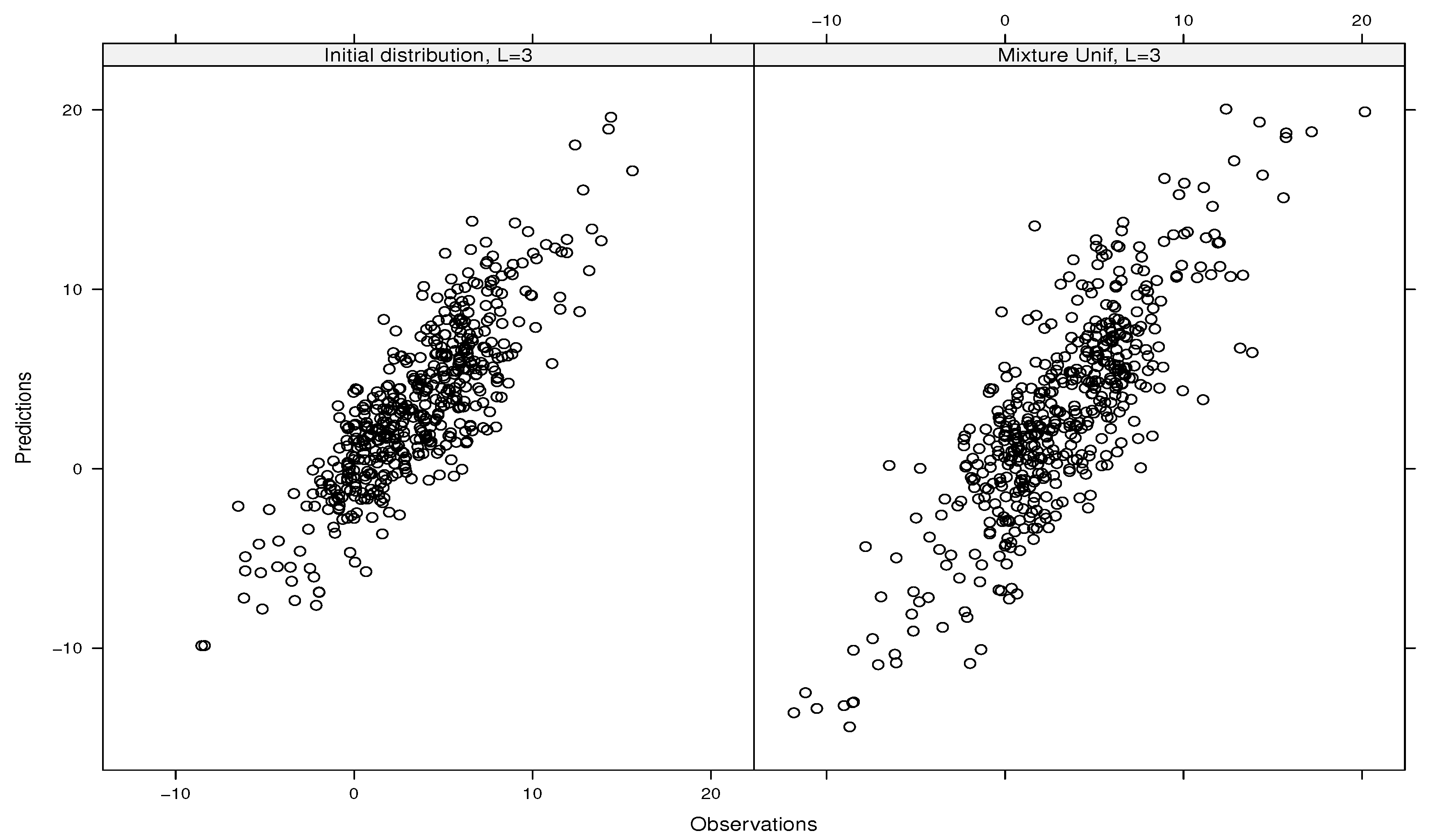
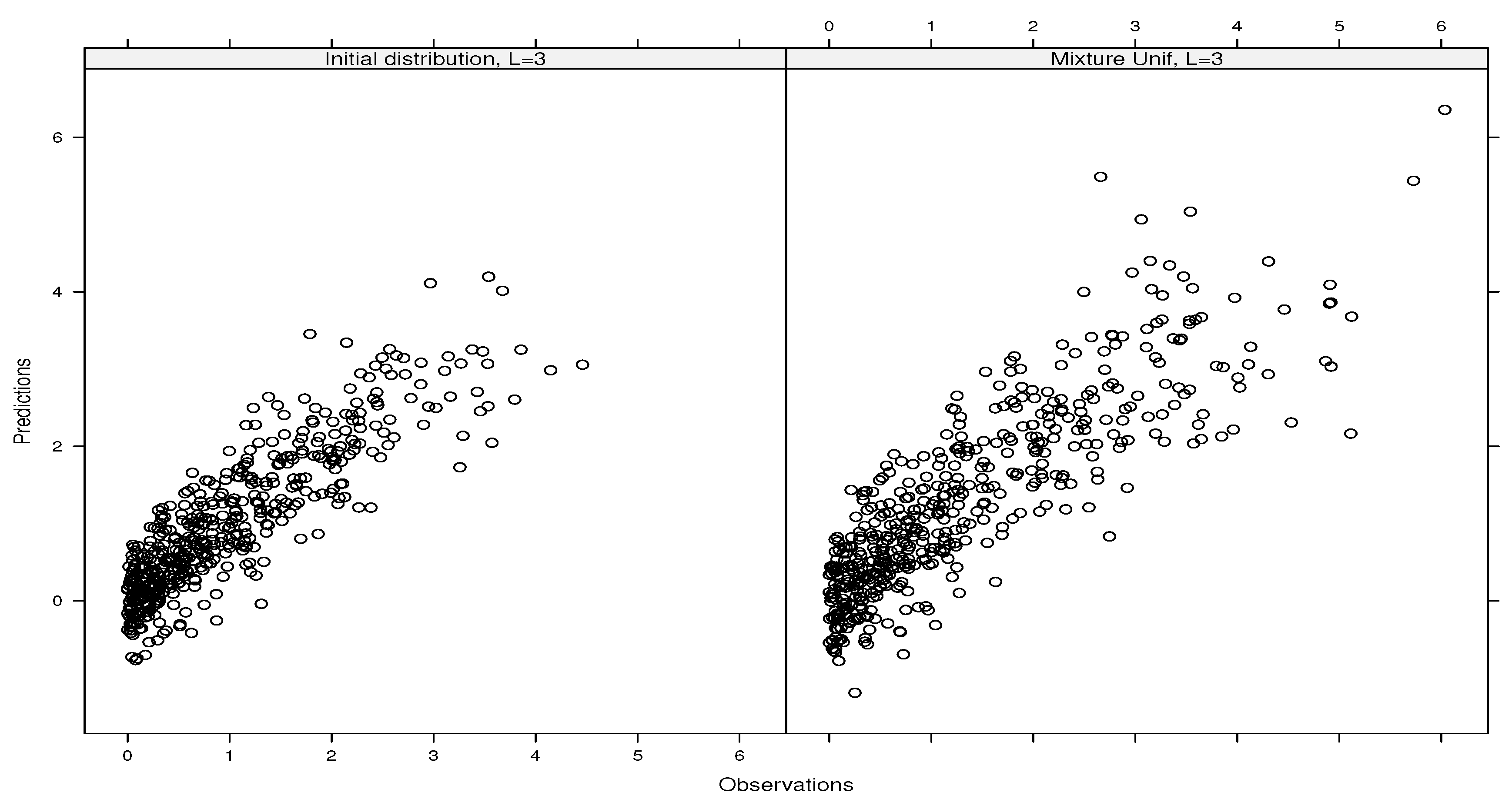
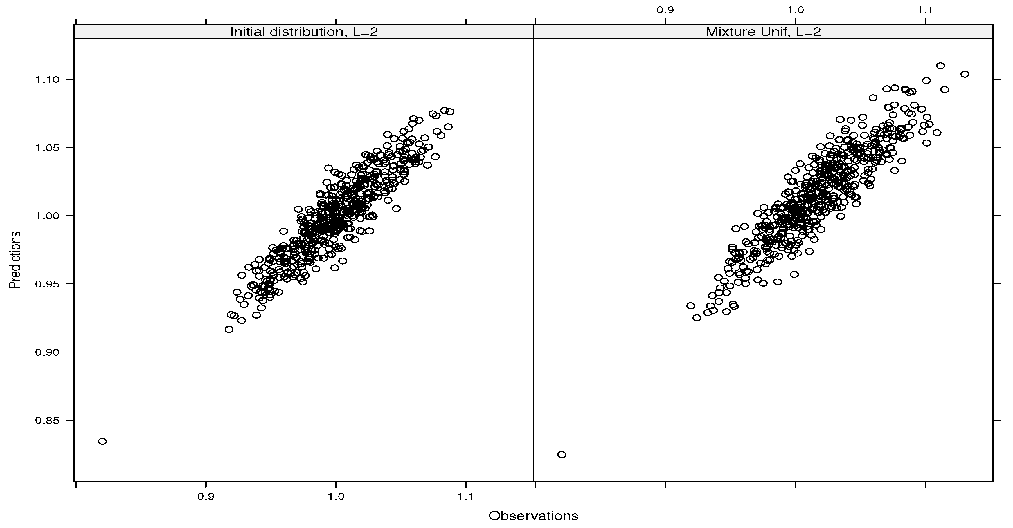
5. Application: Heat Diffusion Models with Stochastic Initial Conditions

We deployed our emulators to approximate a high-dimensional model defined by the one-dimensional (1-D) diffusion PDE with stochastic initial conditions, that is,

$$\left\{\begin{array}{cc}{\displaystyle \frac{\partial f}{\partial t}}-D{\displaystyle \frac{{\partial }^{2}f}{{\partial }^{2}x}}=0,\hfill & \hfill x\in ]0,1[,t\in [0,T]\\ f(x,t=0)=Z\left(x\right)\hfill & \hfill x\in [0,1]\\ f(x=0,t)=0,f(x=1,t)=1,\hfill & \hfill t\in [0,T]\end{array}\right.,$$

where $D=0.0011$ represents the diffusion coefficient. The quantity of interest (QoI) is given by $J\left(Z\left(x\right)\right):={\displaystyle \frac{1}{2}}{\int }_0^T{\int }_0^{10}{\left(f(x,t)\right)}^{2}dxdt$. The spatial discretization consists of subdividing the spatial domain, $[0,1]$, into d equally-sized cells, leading to d initial conditions or inputs, that is, $Z\left(x_j\right)$ with $j=1,\dots ,d$. We assume that the $d=50$ inputs are independent, and $X_j:=Z\left(x_j\right)\sim \mathcal{U}\left(sin\left(2\pi x_j\right)-1.96,sin\left(2\pi x_j\right)+1.96\right)$. A time step of $0.025$ was considered, starting from 0 up to $T=5$.

It is known [12] that the exact gradient can be computed as follows: ${\nabla }_{Z}J\left(Z\left(x\right)\right)=f^a(x,0)$, where $f^a(x,0)$ stands for the adjoint model of f evaluated at $(x,t=0)$. Note that only one evaluation of such a function is needed to obtain the gradient of the QOI. The adjoint model is given by (see ref. [12])

$$\left\{\begin{array}{cc}-{\displaystyle \frac{\partial f^a}{\partial t}}-D{\displaystyle \frac{{\partial }^2{f}^a}{{\partial }^{2}x}}=f,\hfill & \hfill x\in ]0,1[,t\in [0,T]\\ f^a(x=0,t)=f^a(x=1,t)=0,\hfill & \hfill t\in [0,T]\\ f^a(x,T)=0,\hfill & \hfill x\in [0,1]\end{array}\right..$$

The values of the hyper-parameters derived in this paper (considered at the beginning of Section 4) were used to compute the results below. Using the exact values of the gradient (i.e., $f^a(x,0)$), we computed the main indices ($S_j$s) and the upper bounds of the total indices ($U{B}_j$s) (see Figure 4, top-left panel). It appears that the upper bounds are almost equal to the main indices, showing the absence of interactions. This information is confirmed by the fact that ${\sum }_{j=1}^{d=50}{S}_j=1.09$, leading to $d_0=1$. Based on this information, Figure 4 (top-right panel) depicts the predictions versus the observations (simulated outputs) using the derivative-based emulator with all the first-order partial derivatives. In the same sense, Figure 4 (bottom-left panel) depicts the observations versus predictions by including only the ANOVA components for which $U{B}_j>0.01$, that is, 37 components. Both results are close together and are in line with the observations. Finally, Figure 4 (bottom-right panel) shows the observations versus predictions for derivative-free emulators using only the components for which $U{B}_j>0.01$. It turns out that our emulators provide reliable estimations. As expected (see MSEs), the derivative-based emulator using exact values of derivatives performs better.

6. Conclusions

In this paper, we have proposed simple, practical, and sound emulators of simulators or estimators of functions using either the available derivatives and distribution functions of inputs or derivative-free methods, such as stochastic approximations. Since our emulators or estimators rely exactly on Db-ANOVA, Sobol’s indices and their upper bounds were used to derive the appropriate structures of such emulators so as to reduce epistemic uncertainty. The derivative-based and derivative-free emulators reach the parametric rate of convergence (i.e., $\mathsf{O}\left(N^{-1}\right)$) and have dimension-free biases. Moreover, the former emulators enjoy dimension-free MSEs when all cross-partial derivatives are available and, therefore, can cope with higher-dimensional models. However, the MSEs of the derivative-free estimators depend on dimensionality, and we have shown that the stability and accuracy of such emulators require about $N\approx {(d+1)}^d$ model runs for full emulators and about $N\approx min\left(d^{2d_0},2^d{d}^{d_0}\right)$ runs for unbiased, truncated emulators of order $d_0$.

To be able to deploy our emulators in practice, we have provided the best known values for the hyper-parameters needed. The numerical results have revealed that our emulators provide efficient predictions of models once the adequate structures of such models are used. While such results are promising, further improvements are going to be investigated in our next works by i) considering distributions of $V_j$s that may help in reducing the dimensionality in MSEs, ii) taking into account the discrepancy errors by using the output observations (rather than their mean only), and iii) considering local emulators. It is also worth investigating adaptations of such methods in the presence of empirical data.

References

1. Max, D.; Morris, T.J.M.; Ylvisaker, D. Bayesian Design and Analysis of Computer Experiments: Use of Derivatives in Surface Prediction. Technometrics 1993, 35, 243–255. [Google Scholar]
2. Solak, E.; Murray-Smith, R.; Leithead, W.; Leith, D.; Rasmussen, C. Derivative observations in Gaussian process models of dynamic systems. Adv. Neural Inf. Process. Syst. 2002, 15, 1–8. [Google Scholar]
3. Le Dimet, F.X.; Talagrand, O. Variational algorithms for analysis and assimilation of meteorological observations: Theoretical aspects. Tellus A Dyn. Meteorol. Oceanogr. 1986, 38, 97–110. [Google Scholar] [CrossRef]
4. Le Dimet, F.X.; Ngodock, H.E.; Luong, B.; Verron, J. Sensitivity analysis in variational data assimilation. J. Meteorol. Soc. Jpn. 1997, 75, 245–255. [Google Scholar] [CrossRef]
5. Cacuci, D.G. Sensitivity and Uncertainty Analysis—Theory; Chapman & Hall/CRC: Boca Raton, FL, USA, 2005. [Google Scholar]
6. Gunzburger, M.D. Perspectives in Flow Control and Optimization; SIAM: Philadelphia, PA, USA, 2003. [Google Scholar]
7. Borzi, A.; Schulz, V. Computational Optimization of Systems Governed by Partial Differential Equations; SIAM: Philadelphia, PA, USA, 2012. [Google Scholar]
8. Ghanem, R.; Higdon, D.; Owhadi, H. Handbook of Uncertainty Quantification; Springer International Publishing: Berlin/Heidelberg, Germany, 2017. [Google Scholar]
9. Agarwal, A.; Dekel, O.; Xiao, L. Optimal Algorithms for Online Convex Optimization with Multi-Point Bandit Feedback. In Proceedings of the COLT, Haifa, Israel, 27–29 June 2010; Citeseer: Princeton, NJ, USA, 2010; pp. 28–40. [Google Scholar]
10. Bach, F.; Perchet, V. Highly-Smooth Zero-th Order Online Optimization. In Proceedings of the 29th Annual Conference on Learning Theory, New York, NY, USA, 23–26 June 2016; Volume 49, pp. 257–283. [Google Scholar]
11. Akhavan, A.; Pontil, M.; Tsybakov, A.B. Exploiting higher order smoothness in derivative-free optimization and continuous bandits. In Proceedings of the NIPS ’20: Proceedings of the 34th International Conference on Neural Information Processing Systems, Vancouver, BC, Canada, 6–12 December 2020. [Google Scholar]
12. Lamboni, M. Optimal and Efficient Approximations of Gradients of Functions with Nonindependent Variables. Axioms 2024, 13, 426. [Google Scholar] [CrossRef]
13. Lamboni, M. Optimal Estimators of Cross-Partial Derivatives and Surrogates of Functions. Stats 2024, 7, 1–22. [Google Scholar] [CrossRef]
14. Chkifa, A.; Cohen, A.; DeVore, R.; Schwab, C. Sparse adaptive Taylor approximation algorithms for parametric and stochastic elliptic PDEs. ESAIM Math. Model. Numer. Anal. 2013, 47, 253–280. [Google Scholar] [CrossRef]
15. Patil, P.; Babaee, H. Reduced-Order Modeling with Time-Dependent Bases for PDEs with Stochastic Boundary Conditions. SIAM/ASA J. Uncertain. Quantif. 2023, 11, 727–756. [Google Scholar] [CrossRef]
16. Sobol, I.M.; Kucherenko, S. Derivative based global sensitivity measures and the link with global sensitivity indices. Math. Comput. Simul. 2009, 79, 3009–3017. [Google Scholar] [CrossRef]
17. Kucherenko, S.; Rodriguez-Fernandez, M.; Pantelides, C.; Shah, N. Monte Carlo evaluation of derivative-based global sensitivity measures. Reliab. Eng. Syst. Saf. 2009, 94, 1135–1148. [Google Scholar] [CrossRef]
18. Lamboni, M.; Iooss, B.; Popelin, A.L.; Gamboa, F. Derivative-based global sensitivity measures: General links with Sobol’ indices and numerical tests. Math. Comput. Simul. 2013, 87, 45–54. [Google Scholar] [CrossRef]
19. Roustant, O.; Fruth, J.; Iooss, B.; Kuhnt, S. Crossed-derivative based sensitivity measures for interaction screening. Math. Comput. Simul. 2014, 105, 105–118. [Google Scholar] [CrossRef]
20. Roustant, O.; Barthe, F.; Iooss, B. Poincar inequalities on intervals—Application to sensitivity analysis. Electron. J. Statist. 2017, 11, 3081–3119. [Google Scholar] [CrossRef]
21. Lamboni, M. Derivative-based integral equalities and inequality: A proxy-measure for sensitivity analysis. Math. Comput. Simul. 2021, 179, 137–161. [Google Scholar] [CrossRef]
22. Lamboni, M. Weak derivative-based expansion of functions: ANOVA and some inequalities. Math. Comput. Simul. 2022, 194, 691–718. [Google Scholar] [CrossRef]
23. Lamboni, M.; Kucherenko, S. Multivariate sensitivity analysis and derivative-based global sensitivity measures with dependent variables. Reliab. Eng. Syst. Saf. 2021, 212, 107519. [Google Scholar] [CrossRef]
24. Krige, D.G. A Statistical Approaches to Some Basic Mine Valuation Problems on the Witwatersrand. J. Chem. Metall. Soc. S. Afr. 1951, 52, 119–139. [Google Scholar]
25. Currin, C.; Mitchell, T.; Morris, M.; Ylvisaker, D. Bayesian Prediction of Deterministic Functions, with Applications to the Design and Analysis of Computer Experiments. J. Am. Stat. Assoc. 1991, 86, 953–963. [Google Scholar] [CrossRef]
26. Oakley, J.E.; O’Hagan, A. Probabilistic sensitivity analysis of complex models: A Bayesian approach. J. R. Stat. Soc. Ser. B Stat. Methodol. 2004, 66, 751–769. [Google Scholar] [CrossRef]
27. Conti, S.; O’Hagan, A. Bayesian emulation of complex multi-output and dynamic computer models. J. Stat. Plan. Inference 2010, 140, 640–651. [Google Scholar] [CrossRef]
28. Kennedy, M.C.; O’Hagan, A. Bayesian calibration of computer models. J. R. Stat. Soc. Ser. B Stat. Methodol. 2001, 63, 425–464. [Google Scholar] [CrossRef]
29. Xiu, D.; Karniadakis, G. The Wiener-Askey polynomial chaos for stochastic di eren-tial equations. Siam J. Sci. Comput. 2002, 24. [Google Scholar] [CrossRef]
30. Ghanem, R.G.; Spanos, P.D. Stochastic Finite Elements: A Spectral Approach; Springer: New York, NY, USA, 1991; pp. 1–214. [Google Scholar]
31. Sudret, B. Global sensitivity analysis using polynomial chaos expansions. Reliab. Eng. Syst. Saf. 2008, 93, 964–979. [Google Scholar] [CrossRef]
32. Wahba, G. Spline Models for Observational Data; Society for Industrial and Applied Mathematics: Philadelphia, PA, USA, 1990. [Google Scholar] [CrossRef]
33. Wong, R.K.W.; Storlie, C.B.; Lee, T.C.M. A Frequentist Approach to Computer Model Calibration. J. R. Stat. Soc. Ser. B Stat. Methodol. 2016, 79, 635–648. [Google Scholar] [CrossRef]
34. Friedman, J.H.; Popescu, B.E. Predictive learning via rule ensembles. Ann. Appl. Stat. 2008, 2, 916–954. [Google Scholar] [CrossRef]
35. Horiguchi, A.; Pratola, M.T. Estimating Shapley Effects in Big-Data Emulation and Regression Settings using Bayesian Additive Regression Trees. arXiv 2024, arXiv:2304.03809. [Google Scholar]
36. Migliorati, G.; Nobile, F.; Schwerin, E.; Tempone, R. Analysis of Discrete L2 Projection on Polynomial Spaces with Random Evaluations. Found. Comput. Math. 2014, 14, 419–456. [Google Scholar]
37. Hampton, J.; Doostan, A. Coherence motivated sampling and convergence analysis of least squares polynomial Chaos regression. Comput. Methods Appl. Mech. Eng. 2015, 290, 73–97. [Google Scholar] [CrossRef]
38. Cohen, A.; Davenport, M.A.; Leviatan, D. On the stability and accuracy of least squares approximations. arXiv 2018, arXiv:math.NA/1111.4422. [Google Scholar] [CrossRef]
39. Tsybakov, A. Introduction to Nonparametric Estimation; Springer: New York, NY, USA, 2009. [Google Scholar]
40. Zemanian, A. Distribution Theory and Transform Analysis: An Introduction to Generalized Functions, with Applications; Dover Books on Advanced Mathematics; Dover Publications: Garden City, NY, USA, 1987. [Google Scholar]
41. Strichartz, R. A Guide to Distribution Theory and Fourier Transforms; Studies in advanced mathematics; CRC Press: Boca Raton, FL, USA, 1994. [Google Scholar]
42. Caflisch, R.E.; Morokoff, W.J.; Owen, A.B. Valuation of mortgage-backed securities using Brownian bridges to reduce effective dimension. J. Comput. Financ. 1997, 1, 27–46. [Google Scholar] [CrossRef]
43. Owen, A. The dimension distribution and quadrature test functions. Stat. Sin. 2003, 13, 1–17. [Google Scholar]
44. Rabitz, H. General foundations of high dimensional model representations. J. Math. Chem. 1999, 25, 197–233. [Google Scholar] [CrossRef]
45. Kuo, F.; Sloan, I.; Wasilkowski, G.; Woźniakowski, H. On decompositions of multivariate functions. Math. Comput. 2010, 79, 953–966. [Google Scholar] [CrossRef]
46. Alatawi, M.S.; Martinucci, B. On the Elementary Symmetric Polynomials and the Zeros of Legendre Polynomials. J. Math. 2022, 1–9. [Google Scholar] [CrossRef]
47. Arafat, A.; El-Mikkawy, M. A Fast Novel Recursive Algorithm for Computing the Inverse of a Generalized Vandermonde Matrix. Axioms 2023, 12, 27. [Google Scholar] [CrossRef]
48. Rawashdeh, E. A simple method for finding the inverse matrix of Vandermonde matrix. Mathematiqki Vesnik 2019, 71, 207–213. [Google Scholar]
49. Homma, T.; Saltelli, A. Importance measures in global sensitivity analysis of nonlinear models. Reliab. Eng. Syst. Saf. 1996, 52, 1–17. [Google Scholar] [CrossRef]
Figure 1. Predictions versus simulated outputs (observations) for Ishigami’s function.
Stats 08 00024 g001
Figure 2. Predictions versus simulated outputs (observations) for the g-function of type A.
Stats 08 00024 g002
Figure 3. Predictions versus simulated outputs (observations) for the g-function of type B.
Stats 08 00024 g003
Figure 4. Main indices (∘) and upper bounds of total indices (+) of d = 50 inputs (top-left panel); observations versus predictions using either derivative-based emulators (see the top-right panel when including all components and the bottom-left panel for all other cases) or derivative-free emulators (bottom-right panel).
Stats 08 00024 g004
Disclaimer/Publisher’s Note: The statements, opinions and data contained in all publications are solely those of the individual author(s) and contributor(s) and not of MDPI and/or the editor(s). MDPI and/or the editor(s) disclaim responsibility for any injury to people or property resulting from any ideas, methods, instructions or products referred to in the content.