Article

A Bayesian One-Sample Test for Proportion

1
Department of Mathematical & Computational Sciences, University of Toronto Mississauga, Mississauga, ON L5L 1C6, Canada
2
Department of Statistics & Actuarial Science, University of Hong Kong, Pok Fu Lam, Hong Kong
3
Department of Mathematics & Statistics, McMaster University, 1280 Main St. W, Hamilton, ON L8S 4L8, Canada
4
Department of Mathematics & Department of Statistical Sciences, University of Toronto St. George, 27 King’s College Circle, Toronto, ON M5S 1A4, Canada
*
Author to whom correspondence should be addressed.
Stats 2022, 5(4), 1242-1253; https://doi.org/10.3390/stats5040075
Submission received: 26 October 2022 / Revised: 27 November 2022 / Accepted: 28 November 2022 / Published: 1 December 2022

Abstract

:
This paper deals with a new Bayesian approach to the one-sample test for proportion. More specifically, let x = ( x 1 , , x n ) be an independent random sample of size n from a Bernoulli distribution with an unknown parameter θ . For a fixed value θ 0 , the goal is to test the null hypothesis H 0 : θ = θ 0 against all possible alternatives. The proposed approach is based on using the well-known formula of the Kullback–Leibler divergence between two binomial distributions chosen in a certain way. Then, the difference of the distance from a priori to a posteriori is compared through the relative belief ratio (a measure of evidence). Some theoretical properties of the method are developed. Examples and simulation results are included.

1. Introduction

The one-sample test for proportion is a topic that is taught in most introductory statistics courses. Let x = ( x 1 , , x n ) be an independent random sample of size n from a Bernoulli distribution with unknown parameter θ , where θ [ 0 , 1 ] . The interest is to test the null hypothesis H 0 : θ = θ 0 , where θ 0 is a known value.
In this problem, within the classical frequentist framework, the approximate z-test is commonly used for testing H 0 . Specifically, if n θ 0 5 and n ( 1 θ 0 ) 5 (i.e., a large-sample test), the test statistic is given by
z = θ ^ θ 0 θ 0 ( 1 θ 0 ) / n ,
where θ ^ = i = 1 n x i / n represents the maximum likelihood estimator under H 0 . For example, to test H 0 against the alternative hypothesis H 1 : θ θ 0 , the two-sided p-value is equal to 2 P ( Z > | z | ) , where Z has the standard normal distribution. Then, H 0 is rejected if the p-value is less than a given significance level α . As for a small-sample test, the exact binomial distribution (rather than a normal approximation) is typically used. We refer the reader to Chapter 12 of [1] for general methods of dealing with hypothesis testing problems.
A standard alternative method to the earlier procedures is the Bayesian approach by means of the Bayes factor [2,3]. This requires the specification of prior distributions for parameters. It is noticed that most of the Bayesian methods in this area are presented for comparing the proportion in two-sample problems. For instance, ref. [4] proposed an approximation for the Bayes factor to test the equality of two binomial proportions. Furthermore, ref. [5] provided some recommendations for using Bayes factors in testing the equality of two proportions to improve the sensitivity of the test. Several studies can also be found in the literature on developing the Bayesian two-sample proportion test in contingency tables for testing the independence between rows and columns. See, for example, ref. [6] and the references therein.
For the one-sample problem, ref. [7] used an improper prior for the proportion in clinical trials. They computed the probability of being under the null and alternative hypotheses and then compared them to decide whether to accept the null hypothesis. Ref. [8] developed the BayesFactor R package, which can be used to compute the Bayes factor for several research designs and hypotheses including a test for one-sample proportion. Ref. [9] discussed this problem in detail based on a direct computation of the relative belief ratio. In this paper, a different Bayesian approach to the one-sample test for proportion is proposed. First, to avoid a prior-data conflict (see Section 2), the uniform [ 0 , 1 ] is placed as a prior on the true proportion, then the Kullback–Leibler divergence between two binomial distributions (sampling and hypothesized distributions selected in an appropriate way). The difference of the distance from a priori to a posteriori is compared such that, if the posterior distribution is more concentrated around the hypothesized distribution than the prior distribution, then there is evidence in favor of the null hypothesis. Furthermore, if the posterior distribution is less concentrated, then it indicates evidence against the null hypothesis. This comparison is made via a relative belief ratio, which measures the evidence in the observed data for or against the null hypothesis. We also discuss a measure of the strength of this evidence, and therefore, the proposed test is completely based on a direct measure of statistical evidence.
We highlight here some key motivations of the proposed technique. First, it is simple, and the computations are straightforward. Second, unlike the classical approach, it gives evidence in favor of the null hypothesis and does not require choosing the significance level. Third, it avoids any possibility of the prior for prior-data conflict and, hence, provides robustness in the analysis [10]. Fourth, the proposed method uses the relative belief and computes the strength separately, and it has been proven to work as a calibration of the relative belief [9]. Fifth, similar to the exact binomial test, the proposed test works for small sample sizes. Lastly, it can be extended to the case of the equality of k independent sample binomial proportions.
The remainder of this paper is organized as follows. Inferences using the relative belief ratio are introduced in Section 2. In Section 3, a Bayesian test is proposed. In this section, we also cover checking for prior-data conflict, prior elicitation, and the prior for bias. In Section 4, we consider several examples to illustrate the approach. A comparison with other methods is also considered in this section. Finally, some concluding remarks are given in Section 5.

2. Inferences Using Relative Belief

The relative belief ratio was developed in [9], and it has become a widely used tool in the theory of Bayesian statistical hypothesis testing. For some references, see, for example, [11,12,13,14]. Suppose a statistical model is given by the density function { f θ ( x ) : θ Θ } with respect to Lebesgue measure on the parameter space Θ . Let π ( θ ) be a prior on Θ . After observing the data x, the posterior distribution of θ is given by the density π ( θ | x ) = f θ ( x ) π ( θ ) m ( x ) , where m ( x ) = Θ f θ ( x ) π ( θ ) d θ . If the interest is to make an inference about the parameter θ , when π ( · ) and π ( · | x ) are continuous at θ , the relative belief ratio for a hypothesized value θ 0 of θ is
R B ( θ 0 | x ) = π ( θ 0 | x ) π ( θ 0 ) .
If π ( · ) and π ( · | x ) are discrete, the relative belief ratio is defined through limits [9]. Clearly, (1) measures how beliefs have changed such that θ 0 is the true value from a priori to a posteriori. Accordingly, R B ( θ 0 | x ) is a measure of evidence that θ 0 is the true value. If R B ( θ 0 | x ) > 1 , then the probability of θ 0 being the true value increases from a priori to a posteriori, and so, there is evidence based on the data that θ 0 is the true value; therefore, there is evidence in favor of θ 0 . If R B ( θ 0 | x ) < 1 , then the probability of θ 0 being the true value decreases from a priori to a posteriori. Thus, the data provide evidence against θ 0 being the true value. When R B ( θ 0 | x ) = 1 , then there is no evidence either way.
Let T denote a minimal sufficient statistic for { f θ : θ Θ } with density f θ T ( t ) and m T ( t ) = Θ f θ T ( t ) π ( θ ) d θ . Ref. [15] showed that
R B ( θ 0 | x ) = f θ 0 T ( x ) m T ( T ( x ) ) = f θ 0 ( x ) ) m ( x ) .
The relationship in (2) is known as the Savage–Dickey ratio.
The next step after computing (2) is to calibrate whether this value indicates strong or weak evidence for or against H 0 : θ = θ 0 . A standard calibration of R B ( θ 0 | x ) is obtained by computing the following probability [9]:
S t r ( θ 0 | x ) = Π ( R B ( θ | x ) R B ( θ 0 | x ) | x ) = { θ Θ : R B ( θ | x ) R B ( θ 0 | x ) } π ( θ | x ) d θ .
Here, Π ( · | x ) is the posterior cumulative distribution function with posterior density π ( · | x ) . As S t r ( θ 0 | x ) represents the posterior probability that the true value of θ has a relative belief ratio of at most the relative belief ratio at θ 0 , when R B ( θ 0 | x ) < 1 , a small value for S t r ( θ 0 | x ) gives strong evidence against H 0 (most of the values of θ have relative belief ratios greater than the relative belief ratio at θ 0 ). On the other side, if R B ( θ 0 | x ) > 1 , a large value for S t r ( θ 0 | x ) gives strong evidence in favor of θ 0 (most of the values of θ have relative belief ratios smaller than the relative belief ratio at θ 0 ), while a small value of S t r ( θ 0 | x ) indicates weak evidence in favor of θ 0 .
Another basic issue when dealing with Bayesian inference methods is the possibility to bias the analysis by the prior. To assess any possible bias, following [9], when H 0 is true, the bias against H 0 : θ = θ 0 can be measured by computing the prior probability:
M T ( R B ( θ 0 | x ) 1 | θ 0 ) ,
where M T ( · | θ 0 ) denotes the prior predictive distribution of T when the true value is θ 0 . Large values of (4) imply there is a bias against H 0 and there is a concern about any evidence against H 0 . On the other side, the bias in favor of H 0 is given by the prior probability
M T ( R B ( θ 0 | x ) 1 | θ 0 )
for values θ 0 θ 0 such that the difference between θ 0 and θ 0 represents the smallest difference of practical importance. When the bias in favor is large, then there is evidence in favor of H 0 . As a result, any evidence in favor of H 0 is not convincing. For a fixed prior, both biases decrease as the sample size increases.
Another concern that appears in Bayesian analysis is whether a chosen prior may be strongly contradicted by the data [9]. A possible contradiction between the data and the prior is known as a prior-data conflict. A common method for checking the prior was developed by [16], which involves computing the probability:
M T m T ( t ) m T ( T ( x ) ) ,
where T is a minimal sufficient statistic of the model and M T is the prior predictive probability distribution of T with density m T and is given by M T ( A ) = A Θ π ( θ ) f θ T ( t ) d θ d t = A m T ( t ) d t . If (6) is small, then T ( x ) lies in a region of low prior probability, such as a tail or anti-mode, which indicates a conflict. Furthermore, if (6) is large, then prior-data conflict should not be an issue. For different methods of checking prior-data conflict, see [17]. Furthermore, for relevant robustness results of inferences based on the relative belief ratio, see [10,18], where a strong connection between robustness and prior-data conflict is found.

3. One-Sample Bayesian Test for Proportion

3.1. The Approach

The proposed test is based on using the Kullback–Leibler (KL) distance. The KL distance between two discrete cumulative distribution functions (cdfs) P and Q defined on the same probability space with corresponding probability mass functions (pmfs) p and q (with respect to the counting measure) is defined by
d ( P , Q ) = x φ p ( x ) log p ( x ) q ( x ) .
It is well known that d K L ( P , Q ) 0 , and the equality holds if and only if p = q . However, it is not symmetric and does not satisfy the triangle inequality [19]. For example, if P and Q are the cdfs of binomial ( n , θ ) and binomial ( n , θ 0 ) , respectively, then the KL divergence between P and Q is given by
d ( P , Q ) = n θ log θ θ 0 + ( 1 θ ) log 1 θ 1 θ 0 .
As d ( P , Q ) = 0 if and only if θ = θ 0 , testing H 0 : θ = θ 0 is equivalent to testing H 0 : d ( P , Q ) = 0 . For the proposed Bayesian approach, to test H 0 : θ = θ 0 , let Beta( α 0 , β 0 ) be the prior of θ . Then, the posterior distribution of θ given x = ( x 1 , , x n ) is Beta( α x , β x ), where α x = α 0 + i = 1 n x i and β x = β 0 + n i = 1 n x i . If θ Beta ( α 0 , β 0 ) , we denote d ( P , Q ) by D = d prior ( P , Q ) , and if θ Beta ( α x , β x ) , then we write D x = d post ( P , Q ) . Note that, as n , by the weak law of large numbers, 𝔼 ( θ | x ) = α x α x + β x = α 0 + i = 1 n x i n + α 0 + β 0 p θ true , the true population proportion. Thus, by (7), if H 0 is true, we have D x a . s . 0 . On the other hand, if H 0 is not true, then
D x a . s . c ,
where c > 0 . It follows that, if H 0 is true, then that distribution of D x should be concentrated about 0 more than D. Therefore, the proposed test is constructed based on a comparison of the distribution of D and D x about 0 via the relative belief ratio:
R B D ( 0 | x ) = π D ( 0 | x ) π D ( 0 ) ,
where π D ( 0 ) and π D ( 0 | x ) are the probability density functions of D and D x , respectively. If the distribution of D x is more concentrated about 0, then R B D ( 0 | x ) > 1 ; hence, this is evidence in favor of H 0 , while if it is less concentrated about 0, then R B D ( 0 | x ) < 1 , and there is evidence against H 0 . Furthermore, the strength of evidence, whether for or against H 0 , is also computed.
Note that, if d = g ( θ ) denotes the KL divergence function in (7), then
π D ( d ) = 1 g 1 ( g 1 1 ( d ) ) π ( g 1 1 ( d ) ) + 1 g 2 ( g 2 1 ( d ) ) π ( g 2 1 ( d ) ) ,
where g 1 and g 2 are the two parts of g on the left and right sides of θ 0 , respectively. See Figure 1 below.
It follows that
R B D ( 0 | x ) = g 2 ( g 2 1 ( d ) ) g 1 ( g 1 1 ( d ) ) π ( g 1 1 ( d ) | x ) + π ( g 2 1 ( d ) | x ) g 2 ( g 2 1 ( d ) ) g 1 ( g 1 1 ( d ) ) π ( g 1 1 ( d ) ) + π ( g 2 1 ( d ) ) .
Now, as d 0 , g 2 ( g 2 1 ( d ) ) g 1 ( g 1 1 ( d ) ) could 0 , or , or c , c > 0 . In either of theses three cases, R B D ( 0 | x ) = R B ( θ 0 | x ) . The difference between R B D ( 0 | x ) and R B D ( 0 | x ) may occur when d 0 . Accordingly, we develop Algorithm A in Section 3.4 to compute R B D ( 0 | x ) and the corresponding strength S t r D ( 0 | x ) = Π D ( R B ( d | x ) R B ( 0 | x ) | x ) , where Π D ( · | x ) is the cumulative distribution function of D x .

3.2. Checking for Prior-Data Conflict

It is known that T ( x ) = i = 1 n x i is the minimal sufficient statistic for θ . To check for prior-data conflict, we compute that tail probability in (6). If θ Beta ( α 0 , β 0 ) , then the prior prediction function of T ( x ) is given by
m T ( t ) = 0 1 n t θ n ( 1 θ ) n t Γ ( α 0 + β 0 ) Γ ( α 0 ) Γ ( β 0 ) θ α 0 1 ( 1 θ ) β 0 1 d θ = n t Γ ( α 0 + β 0 ) Γ ( α 0 ) Γ ( β 0 ) Γ ( t + α 0 ) Γ ( n t + β 0 ) Γ ( n + α 0 + β 0 ) .
We have
M T m T ( x ) m T ( T ( x ) ) = M T Γ ( t + α 0 ) Γ ( n t + β o ) Γ ( t + 1 ) Γ ( n t + 1 ) Γ ( T ( x ) + α 0 ) Γ ( n T ( x ) + β 0 ) Γ ( T ( x ) + 1 ) Γ ( n T ( x ) + 1 ) .
Clearly, computing (9) should be performed by simulation. For this, generate θ Beta ( α 0 , β 0 ) . Then, generate t Binomial ( n , θ ) . Repeat this many times, and record the proportion of values of m T ( t ) that are less than or equal to m T ( T ( x ) ) giving a Monte Carlo estimate of (9). Clearly, when α 0 = β 0 = 1 , then both sides of the inequality in (9) are equal and the probability is 1. That is, with Beta ( 1 , 1 ) prior (i.e., the uniform [ 0 , 1 ] prior), there is never any prior-data conflict. Accordingly, we choose the prior to be α 0 = β 0 = 1 , which will relax the need to check for prior-data conflict.
The following proposition finds the expected value of D and D x for the uniform [ 0 , 1 ] prior. This proposition could be used, for example, to compare the theoretical and the computed values of D and D x .
Proposition 1.
Let D = d p r i o r ( P , Q ) and D x = d p o s t ( P , Q ) be as defined in Section 3.1:
(i)
If θ Beta ( 1 , 1 ) , then
E ( d prior ( P , Q ) ) = n 1 + log ( θ 0 ( 1 θ 0 ) 2 .
(ii)
If θ Beta ( α x = 1 + i = 1 n x i , β x = 1 + n i = 1 n x i ) , then
E ( d p o s t ( P , Q ) ) = n α x + β x + 1 [ α x ( ψ ( α x + 1 ) ψ ( α x + β x + 1 ) log ( θ 0 ) ) + β x ψ ( β x + 1 ) ψ ( α x + β x + 1 ) log ( 1 θ 0 ) ] ,
where ψ ( x ) = d d x log Γ ( x ) is the digamma function.
Proof. 
Note,
E ( d prior ) = n 0 1 θ log θ θ 0 + ( 1 θ ) log 1 θ 1 θ 0 d θ .
The proof (i) follows by using integration by parts.
To prove (ii), notice that
d post ( P , Q ) = n [ θ log ( θ ) + ( 1 θ ) log ( 1 θ ) θ log ( θ 0 ) ( 1 θ ) log ( 1 θ 0 ) ] .
Now,
E ( θ log ( θ ) ) = 0 1 θ log ( θ ) Γ ( α x + β x ) Γ ( α x ) Γ ( β x ) θ α x 1 ( 1 θ ) β x 1 d θ = Γ ( α x + β x ) Γ ( α x ) Γ ( β x ) 0 1 log ( θ ) θ α x ( 1 θ ) β x 1 d θ = Γ ( α x + β x ) Γ ( α x ) Γ ( β x ) 0 1 α x θ α x ( 1 θ ) β x 1 d θ = Γ ( α x + β x ) Γ ( α x ) Γ ( β x ) α x θ α x ( 1 θ ) β x 1 = α x α x + β x Γ ( α x + β x + 1 ) Γ ( α x + 1 ) Γ ( β x ) α x Γ ( α x + 1 ) Γ ( β x ) Γ ( α x + β x + 1 ) = α x α x + β x α x log Γ ( α x + 1 ) Γ ( β x ) Γ ( α x + β x + 1 ) = α x α x + β x ψ ( α x + 1 ) ψ ( α x + β x + 1 )
Similarly,
E ( 1 θ ) log ( 1 θ ) = β x α x + β x ψ ( β x + 1 ) ψ ( α x + β x + 1 ) .
Furthermore,
E θ log θ 0 = log ( θ 0 ) E ( θ ) = α x α x + β x log ( θ 0 )
and
E ( 1 θ ) log ( 1 θ 0 ) = log ( 1 θ 0 ) E ( 1 θ ) = ( 1 θ 0 ) β x α x + β x
Now, combining the above expectations (12)–(14) in (10) gives the result.    □

3.3. Checking the Prior for Bias

As mentioned in Section 2, there is a need to check if the prior Beta(1,1) induces any bias in the problem. Note that, with this prior, the relative belief ratio R B ( θ | x ) is derived by [9]:
R B ( θ | x ) = Γ ( n + 2 ) θ i = 1 n x i ( 1 θ ) n i = 1 n x i Γ ( 1 + i = 1 n x i ) Γ ( 1 + n i = 1 n x i ) .
The bias against the hypothesis H 0 : θ = θ 0 is measured by computing (4) using R B ( θ | x ) as given in (15). Here, M T ( · | θ 0 ) is the Binomial ( n , θ 0 ) distribution. On the other hand, the bias in favor of the hypothesis H 0 : θ = θ 0 is measured by computing (5) when θ 0 θ 0 is true and R B ( θ 0 | x ) is as defined in (15). Here, M T ( · | θ 0 ) is the Binomial ( n , θ 0 ) distribution. The interpretation of the bias was given in Section 2.
To compute the bias in this problem, it should be performed via simulation. For example, to compute the bias against, generate t Binomial ( n , θ 0 ) , and compute R B ( θ 0 | x ) as defined in (15). Repeat this many times, and record the proportion of values of R B ( θ 0 | x ) that are less than 1. The bias in favor can be estimated similarly.

3.4. The Algorithm

As π D ( · | x ) and π D ( · ) in (8) have no closed forms, the relative belief ratio and the strength need to be estimated via approximation. The following algorithm summarizes the steps required to test H 0 : θ = θ 0 .
Algorithm A (RB test for proportion).
(i)
Generate θ from Beta ( 1 , 1 ) , and compute D.
(ii)
Repeat Step (ii) to obtain a sample of r 1 values of D.
(iii)
Generate θ | x from Beta ( α x = 1 + i = 1 n x i , β x = 1 + n i = 1 n x i ) , and compute D x .
(iv)
Repeat Step (iv) to obtain a sample of r 2 values of D x .
(v)
Compute the relative belief ratio and the strength as follows:
(a)
Let L be a positive number. Let F ^ D denote the empirical cdf of D based on the prior sample in (3), and for i = 0 , , L , let d ^ i / L be the estimate of d i / L , the ( i / L ) -prior quantile of D. Here, d ^ 0 = 0 , and d ^ 1 is the largest value of D. Let F ^ D ( · | x ) denote the empirical cdf based on D x . For d [ d ^ i / L , d ^ ( i + 1 ) / L ) , estimate R B D ( d | x ) = π D ( d | x ) / π D ( d ) by
R B ^ D ( d | x ) = L { F ^ D ( d ^ ( i + 1 ) / L | x ) F ^ D ( d ^ i / L | x ) } ,
the ratio of the estimates of the posterior and prior contents of [ d ^ i / L , d ^ ( i + 1 ) / L ) . Thus, we estimate R B D ( 0 | x ) = π D ( 0 | x ) / π D ( 0 ) by R B ^ D ( 0 | x ) = L F ^ D ( d ^ p 0 | x ) , where p 0 = i 0 / L and i 0 are chosen so that i 0 / L is not too small (typically, i 0 / L 0.05 ) .
(b)
Estimate the strength Π D ( R B D ( d | x ) R B D ( 0 | x ) | x ) by the finite sum:
{ i i 0 : R B ^ D ( d ^ i / L | x ) R B ^ D ( 0 | x ) } ( F ^ D ( d ^ ( i + 1 ) / L | x ) F ^ D ( d ^ i / L | x ) ) .
For fixed L , as r 1 , r 2 , then d ^ i / L converges almost surely to d i / L , and (16) and (17) converge almost surely to R B D ( d | x ) and Π D ( R B D ( d | x ) R B D ( 0 | x ) | x ) , respectively. See [20] for the details.

4. Examples

The approach is illustrated through two examples. In Algorithm A, we set L = 20 and i 0 = 1 . For the sake of comparison, the Bayes factor (BF) of [8] and the p-values of the exact binomial test and the approximate z-test were also considered. The R package BayesFactor was used to compute the BF of [21], while the R functions binom.test() and prop.test() were used to compute the p-values of the exact and the approximate tests, respectively. For these tests, we set α = 0.05 . To interpret the Bayes factor, we used the following rule of thumb introduced by Jefferys in [22]. See also [23]. This scale gives evidence against H 0 . To this end, if B F = 1 , no evidence; 1 < B F < 3 , anecdotal; 3 < B F 10 , moderate; 10 < B F 30 , strong; 30 < B F 100 , very strong; and B F > 100 , extreme. On the other side, if, for example, B F = 0.2 , then 1/0.2 = 45 is interpreted as there is moderate evidence in favor of H 0 .
Example 1.
(Clinical trial; [24]).
A method currently used by doctors to screen women for breast cancer fails to detect cancer in 20% of the women who actually have the disease. A new method has been developed that researchers hope will detect cancer more accurately. This new method was used to screen a random sample of 140 women known to have breast cancer. Of these, the new method failed to detect cancer in 12 women. The researchers want to test if the sample provides evidence that the failure rate of the new method differs from the one currently in use.
First, the bias in the prior is assessed by computing (4) with θ = θ 0 = 0.2 . In this case, the bias against the null hypothesis is 0.2233. On the other hand, the bias in favor of the null hypothesis is measured by computing (5) with θ 0 = 0.2 ± 0.05 , which gives 0.2706 (for θ 0 = 0.25 ) and 0.01737 (for θ 0 = 0.15 ). This shows relatively equal bias either for or against the null hypothesis for the uniform [ 0 , 1 ] prior. The results of the tests are reported in Table 1. In particular, the relative belief ratio of the proposed test is 0.0040, which is less than 1, and the strength is 0.0021, which is close to 0. Hence, there is strong evidence to conclude that the new female breast cancer detection method is better than the used method.
Example 2.
(Production defective; [25]).
A machine in a factory must be repaired if it produces more than 10% defective items among the large lot of items that it produces in a day. A random sample of 100 items from the day’s production contains 15 defective items, and the supervisor says that the machine must be repaired. The goal is to test if the sample provides evidence to support his/her decision.
As in Example 1, the bias in the prior is assessed by computing (4) with θ = θ 0 = 0.1 . In this case, the bias against the null hypothesis is 0.1182. On the other hand, the bias in favor of the null hypothesis is measured by computing (5) with θ 0 = 0.1 ± 0.05 , which gives 0.0504 (for θ 0 = 0.15 ) and 0.0204 (for θ 0 = 0.05 ). This shows an acceptable bias either for or against the null hypothesis for the uniform [ 0 , 1 ] prior. The results of the tests are reported Table 2. As R B = 4.094 > 1 and the strength is 0.406, there is moderate evidence to conclude that the factory produces 10% defective items in a day.

5. Simulation Study

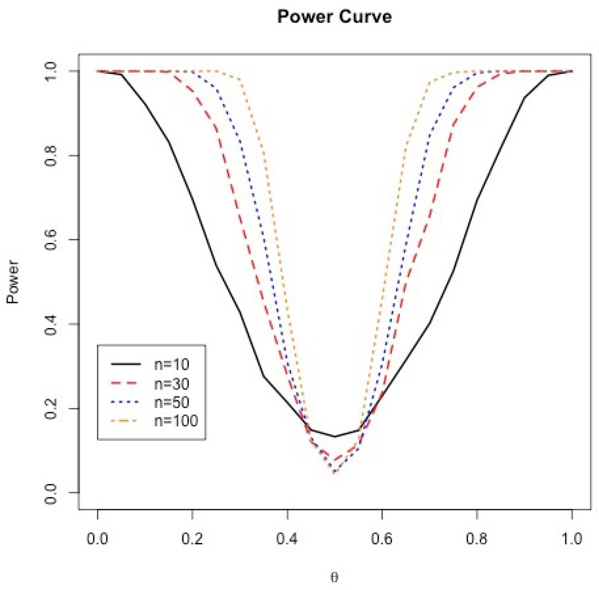
In this section, we run a Monte Carlo simulation study of size 1000 to determine the proportion of false positives (false rejection of the null hypothesis) and the proportion of true positives (true rejection of the null hypothesis) when random data with various sample sizes n { 10 , 30 , 50 , 100 } are generated from the Bernoulli distribution with parameter θ , where θ { 0 , 0.05 , 0.1 , , 0.9 , 0.95 , 1 } . In Figure 2, we plot θ against the proportion of rejecting H 0 : θ = 0.5 (i.e., when R B < 1 ). Figure 2 reveals that when θ is close to 0.5 (i.e., H 0 is true), the proportion of rejecting H 0 is close to 0. However, as θ moves away from 0.5, the curves move toward 1. Furthermore, as the sample size increases, the computed proportions converge faster to the true values.
We also conducted a simulation study to compare the performance of the RB test, the BF test, and the exact and approximate tests. The proportion of rejecting H 0 of the exact and approximate tests is computed by the number of times the p-value is less than 0.05 divided by 1000. For sample sizes n 10 , 30 , 50 , 100 , we generated data from Bernoulli ( θ 0 ) , where θ 0 is given in Table 3 and Table 4. The performance to accept or reject the null hypothesis is reported in these tables. The results in Table 3 and Table 4 show that the RB test performs well.

6. Conclusions

In this paper, a new Bayesian approach to the one-sample test for proportion was developed. The approach is based on using the Kullback–Leibler divergence between two binomial distributions. Then, the change of the distance from a priori to a posteriori was compared through the relative belief. The approach is simple, and the computations are straightforward. Additionally, we anticipate that the approach presented here can be extended to the two-sample and k-sample tests. We leave this extension for future research.

Author Contributions

Conceptualization, L.A.-L.; Methodology, L.A.-L.; Software, K.L.; Validation, Y.C. and Y.W.; Formal analysis, L.A.-L. and F.F.-A.; Investigation, K.L.; Resources, L.A.-L. and F.F.-A.; Data curation, K.L.; Writing—original draft preparation, L.A.-L. and K.L.; Writing—review and editing, F.F.-A. and K.L.; Supervision, L.A.-L.; Project administration, L.A.-L.; Funding acquisition, L.A.-L. All authors have read and agreed to the published version of the manuscript.

Funding

This research received no external funding.

Institutional Review Board Statement

There was no ethical approval is required.

Informed Consent Statement

This study did not involve human or any living organisms.

Data Availability Statement

No dataset had been used.

Acknowledgments

The authors thank the Editor and three anonymous Referees for their important and constructive comments, which led to a significant improvement of the paper, In particular, pointing out the connection between R B D ( 0 | x ) and R B ( θ 0 | x ) in Section 3.1 is highly appreciated.

Conflicts of Interest

There was no conflict of interest.

References

  1. Bain, L.J.; Engelhardt, M. Introduction to Probability and Mathematical Statistics; Duxbury Press: Belmont, CA, USA, 1992; Volume 4. [Google Scholar]
  2. Kass, R.E.; Raftery, A.E. Bayes factors. J. Am. Stat. Assoc. 1995, 90, 773–795. [Google Scholar] [CrossRef]
  3. Rouder, J.N.; Morey, R.D.; Speckman, P.L.; Province, J.M. Default Bayes factors for ANOVA designs. J. Math. Psychol. 2012, 56, 356–374. [Google Scholar] [CrossRef]
  4. Kass, R.E.; Vaidyanathan, S.K. Approximate Bayes factors and orthogonal parameters, with application to testing equality of two binomial proportions. J. R. Stat. Soc. Ser. B (Methodol.) 1992, 54, 129–144. [Google Scholar] [CrossRef]
  5. Dablander, F.; Huth, K.; Gronau, Q.F.; Etz, A.; Wagenmakers, E.J. A puzzle of proportions: Two popular Bayesian tests can yield dramatically different conclusions. Stat. Med. 2022, 41, 1319–1333. [Google Scholar] [CrossRef] [PubMed]
  6. Jamil, T.; Ly, A.; Morey, R.D.; Love, J.; Marsman, M.; Wagenmakers, E.J. Default “Gunel and Dickey” Bayes factors for contingency tables. Behav. Res. Methods 2017, 49, 638–652. [Google Scholar] [CrossRef] [PubMed] [Green Version]
  7. Nieto, A.; Extremera, S.; Gómez, J. Bayesian hypothesis testing for proportions. In Paper SP08; PhUSE: Madrid, Spain, 2011; Available online: https://www.lexjansen.com/phuse/2011/sp/SP08.pdf (accessed on 1 October 2022).
  8. Morey, R.D.; Rouder, J.N.; Jamil, T.; Urbanek, S.; Forner, K.; Ly, A. Package ‘BayesFactor’. 2022. Available online: https://cran.rproject.org/web/packages/BayesFactor/BayesFactor.pdf (accessed on 1 October 2022).
  9. Evans, M. Measuring Statistical Evidence Using Relative Belief; Monographs on Statistics and Applied Probability 144; Taylor & Francis Group, CRC Press: Boca Raton, FL, USA, 2015. [Google Scholar]
  10. Al-Labadi, L.; Evans, M. Optimal robustness results for relative belief inferences and the relationship to prior-data conflict. Bayesian Anal. 2017, 12, 705–728. [Google Scholar] [CrossRef]
  11. Abdelrazeq, I.; Al-Labadi, L.; Alzaatreh, A. On one-sample Bayesian tests for the mean. Statistics 2020, 54, 424–440. [Google Scholar] [CrossRef]
  12. Al-Labadi, L.; Berry, S. Bayesian estimation of extropy and goodness of fit tests. J. Appl. Stat. 2020, 49, 357–370. [Google Scholar] [CrossRef] [PubMed]
  13. Al-Labadi, L.; Patel, V.; Vakiloroayaei, K.; Wan, C. Kullback–Leibler divergence for Bayesian nonparametric model checking. J. Korean Stat. Soc. 2020, 50, 272–289. [Google Scholar] [CrossRef]
  14. Al-Labadi, L. The two-sample problem via relative belief ratio. Comput. Stat. 2021, 36, 1791–1808. [Google Scholar] [CrossRef]
  15. Baskurt, Z.; Evans, M. Hypothesis assessment and inequalities for Bayes factors and relative belief ratios. Bayesian Anal. 2013, 8, 569–590. [Google Scholar] [CrossRef]
  16. Evans, M.; Moshonov, H. Checking for prior-data conflict. Bayesian Anal. 2006, 1, 893–914. [Google Scholar] [CrossRef]
  17. Nott, D.J.; Seah, M.; Al-Labadi, L.; Evans, M.; Ng, H.K.; Englert, B. Using prior expansion for prior-data conflict checking. Bayesian Anal. 2021, 16, 203–231. [Google Scholar] [CrossRef]
  18. Al-Labadi, L.; Asl, F.F. On robustness of the relative belief ratio and the strength of its evidence with respect to the geometric contamination prior. J. Korean Stat. Soc. 2022, 1–15. [Google Scholar] [CrossRef]
  19. Cover, T.M.; Thomas, J.A. Elements of Information Theory, 2nd ed.; Wiley: Hoboken, NJ, USA, 2006. [Google Scholar]
  20. Al-Labadi, L.; Evans, M. Prior-based model checking. Can. J. Stat. 2018, 46, 380–398. [Google Scholar] [CrossRef] [Green Version]
  21. Rouder, J.; Speckman, P.; Sun, D.; Morey, R.; Iverson, G. Bayesian t tests for accepting and rejecting the null hypothesis. Psychon. Bull. Rev. 2009, 16, 225–237. [Google Scholar] [CrossRef] [PubMed]
  22. Jeffreys, H. Theory Probability; Oxford University Press: Oxford, UK, 1961. [Google Scholar]
  23. Raftery, A.E. Bayesian model selection in social research. Sociol. Methodol. 1995, 25, 111–164. [Google Scholar] [CrossRef]
  24. McClave, J.; Sincich, T. Statistics, 13th ed.; Person: Boston, MA, USA, 2017. [Google Scholar]
  25. Wackerly, D.; Mendenhall, W.; Scheaffer, R.L. Mathematical Atatistics with Applications; Cengage Learning: Belmont, CA, USA, 2014. [Google Scholar]
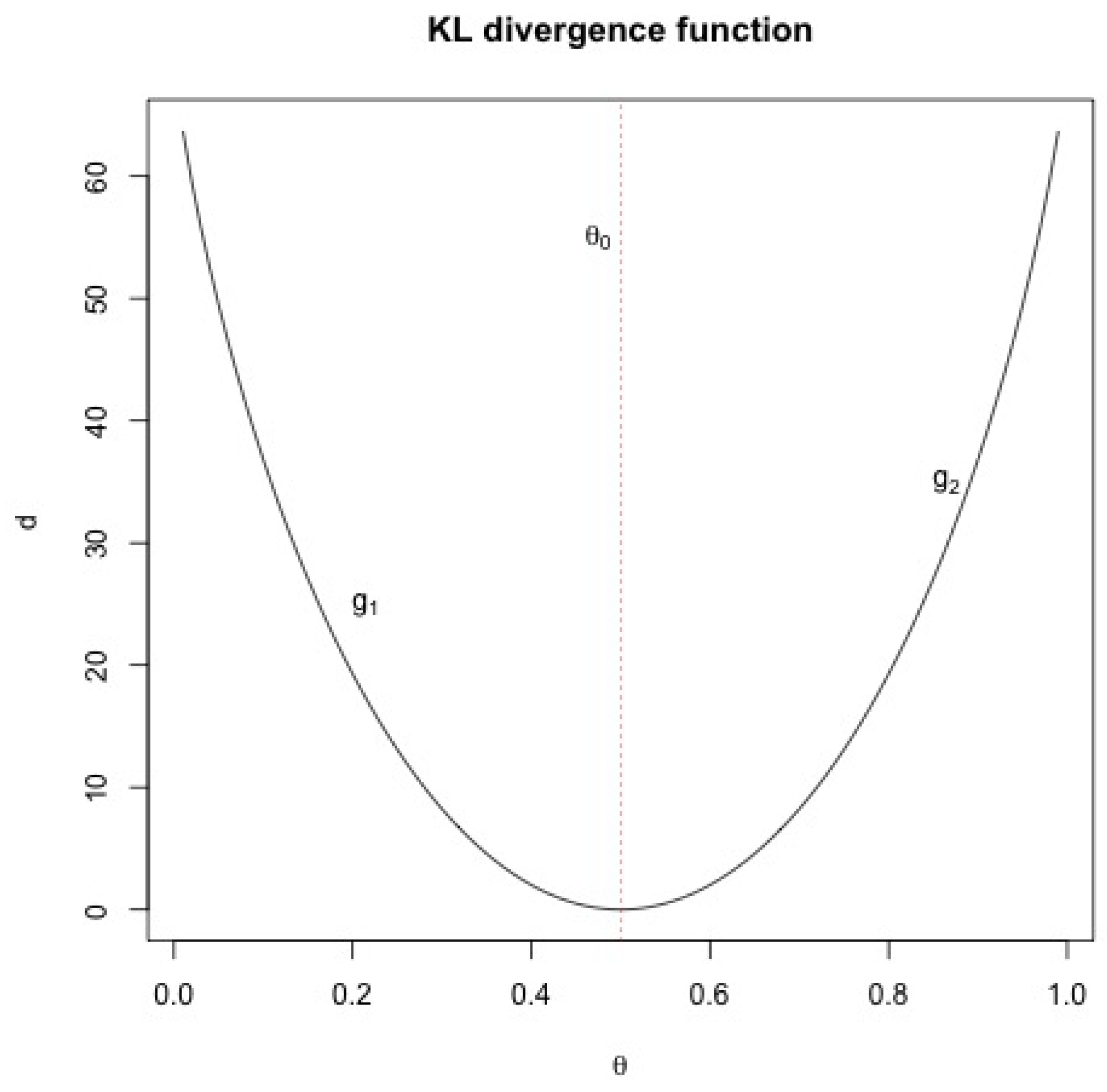
Figure 1. Plot of d = g ( θ ) , the KL divergence function in (7). In the plot, we set θ 0 = 0.5 and n = 10 .
Stats 05 00075 g001
Figure 2. Power curve of the proposed test for various sample sizes n 10 , 30 , 50 , 100 .
Stats 05 00075 g002
Table 1. Test results of Example 1.
TestValuesDecision
RB (strength)0.0400 (0.0021)Strong evidence to reject H 0
RB (strength) using (15)0.0166 (0.0002)Strong evidence to reject H 0
BF167.8429Extreme evidence to reject H 0
p-value (exact)0.0003Reject H 0
p-value (approximate)0.0012Reject H 0
Table 2. Test results of Example 2.
TestValuesDecision
RB (strength)4.094 (0.406)Moderate evidence in favor of H 0
RB (strength) using (15)2.790 (0.1177)Moderate/weak evidence in favor of H 0
BF0.9567Anecdotal evidence for H 0
p-value (exact)0.0962Fail to reject H 0
p-value (approximate)0.1336Fail to reject H 0
Table 3. The proportion of rejecting H 0 out of 1000 replications based on samples of size n = 10 and n = 30 is reported. Here, represents the ratio of false positives for the tests and represents the ratio of the true positives.
n = 10
Proportion RB BF Exact Testz-Test
θ 0 = 0.1 0.922  0.984  0.719  0.835
θ 0 = 0.15 0.832  0.934  0.535  0.689
θ 0 = 0.2 0.696  0.869  0.368  0.530
θ 0 = 0.25 0.539  0.772  0.236  0.381
θ 0 = 0.3 0.428  0.654  0.150  0.256
θ 0 = 0.35 0.276  0.534  0.081  0.161
θ 0 = 0.4 0.214  0.437  0.044  0.098
θ 0 = 0.45 0.149  0.351  0.029  0.062
θ 0 = 0.5 0.133  0.341  0.021  0.050
θ 0 = 0.55 0.148  0.382  0.034  0.062
θ 0 = 0.6 0.230  0.441  0.06  0.098
θ 0 = 0.65 0.315  0.530  0.088  0.161
θ 0 = 0.7 0.402  0.663  0.139  0.256
θ 0 = 0.75 0.526  0.771  0.240  0.381
θ 0 = 0.8 0.694  0.887  0.390  0.530
θ 0 = 0.85 0.818  0.950  0.551  0.689
θ 0 = 0.9 0.937  0.988  0.704  0.835
θ 0 = 0.95 0.990  0.998  0.906  0.943
n = 30
θ 0 = 0.1 1  1  1  0.999
θ 0 = 0.15 0.998  0.999  0.993  0.989
θ 0 = 0.2 0.953  0.974  0.929  0.941
θ 0 = 0.25 0.864  0.884  0.791  0.818
θ 0 = 0.3 0.652  0.712  0.574  0.615
θ 0 = 0.35 0.453  0.502  0.352  0.386
θ 0 = 0.4 0.278  0.297  0.188  0.197
θ 0 = 0.45 0.121  0.153  0.079  0.085
θ 0 = 0.5 0.078  0.101  0.037  0.050
θ 0 = 0.55 0.114  0.152  0.072  0.085
θ 0 = 0.6 0.237  0.297  0.184  0.197
θ 0 = 0.65 0.499  0.489  0.337  0.386
θ 0 = 0.7 0.657  0.721  0.572  0.616
θ 0 = 0.75 0.873  0.891  0.801  0.818
θ 0 = 0.8 0.962  0.979  0.952  0.941
θ 0 = 0.85 0.994  0.998  0.993  0.989
θ 0 = 0.9 1  1  1  0.999
θ 0 = 0.95 1  1  1  1
Table 4. The proportion of rejecting H 0 out of 1000 replications based on samples of size n = 50 and n = 100 is reported. Here, represents the ratio of false positives for the tests and represents the ratio of the true positives.
n = 50
Proportion RB BF Exact Testz-Test
θ 0 = 0.1 1  1  1  1
θ 0 = 0.15 1  1  0.998  1
θ 0 = 0.2 0.998  0.997  0.988  0.995
θ 0 = 0.25 0.959  0.983  0.940  0.959
θ 0 = 0.3 0.834  0.902  0.770  0.829
θ 0 = 0.35 0.605  0.720  0.499  0.577
θ 0 = 0.4 0.309  0.422  0.226  0.296
θ 0 = 0.45 0.131  0.208  0.071  0.109
θ 0 = 0.5 0.051  0.129  0.034  0.050
θ 0 = 0.55 0.105  0.218  0.089  0.109
θ 0 = 0.6 0.306  0.449  0.242  0.296
θ 0 = 0.65 0.589  0.741  0.514  0.577
θ 0 = 0.7 0.848  0.913  0.779  0.829
θ 0 = 0.75 0.961  0.989  0.946  0.959
θ 0 = 0.8 0.996  1  0.995  0.995
θ 0 = 0.85 1  1  1  1
θ 0 = 0.9 1  1  1  1
θ 0 = 0.95 1  1  1  1
n = 100
θ 0 = 0.1 1  1  1  1
θ 0 = 0.15 1  1  1  1
θ 0 = 0.2 1  1  1  1
θ 0 = 0.25 1  1  0.999  0.999
θ 0 = 0.3 0.980  0.99  0.977  0.984
θ 0 = 0.35 0.806  0.91  0.838  0.861
θ 0 = 0.4 0.434  0.629  0.478  0.521
θ 0 = 0.45 0.124  0.230  0.133  0.170
θ 0 = 0.5 0.043  0.092  0.039  0.050
θ 0 = 0.55 0.126  0.248  0.133  0.170
θ 0 = 0.6 0.461  0.633  0.469  0.521
θ 0 = 0.65 0.821  0.907  0.833  0.861
θ 0 = 0.7 0.974  0.989  0.970  0.984
θ 0 = 0.75 0.997  1  1  0.999
θ 0 = 0.8 1  1  1  1
θ 0 = 0.85 1  1  1  1
θ 0 = 0.9 1  1  1  1
θ 0 = 0.95 1  1  1  1
Publisher’s Note: MDPI stays neutral with regard to jurisdictional claims in published maps and institutional affiliations.