Article

A Novel Generalization of Zero-Truncated Binomial Distribution by Lagrangian Approach with Applications for the COVID-19 Pandemic

1
Department of Statistics, Cochin University of Science and Technology, Cochin 682 022, India
2
Department of Mathematics, Université de Caen Basse-Normandie, F-14032 Caen, France
3
Department of Statistics, University College, Thiruvananthapuram 695 034, India
*
Author to whom correspondence should be addressed.
Stats 2022, 5(4), 1004-1028; https://doi.org/10.3390/stats5040060
Submission received: 21 September 2022 / Revised: 26 October 2022 / Accepted: 27 October 2022 / Published: 30 October 2022

Abstract

:
The importance of Lagrangian distributions and their applicability in real-world events have been highlighted in several studies. In light of this, we create a new zero-truncated Lagrangian distribution. It is presented as a generalization of the zero-truncated binomial distribution (ZTBD) and hence named the Lagrangian zero-truncated binomial distribution (LZTBD). The moments, probability generating function, factorial moments, as well as skewness and kurtosis measures of the LZTBD are discussed. We also show that the new model’s finite mixture is identifiable. The unknown parameters of the LZTBD are estimated using the maximum likelihood method. A broad simulation study is executed as an evaluation of the well-established performance of the maximum likelihood estimates. The likelihood ratio test is used to assess the effectiveness of the third parameter in the new model. Six COVID-19 datasets are used to demonstrate the LZTBD’s applicability, and we conclude that the LZTBD is very competitive on the fitting objective.

1. Introduction

Certain discrete distributions whose support is a set of positive integers are known as zero-truncated discrete distributions (ZTDDs). ZTDDs are used in ecology to represent data relating to counts, such as the number of flower heads, fly eggs, European red mites, or the number of times snowshoe hares were collected over seven days. These distributions are also employed in sociology to simulate data such as the size of human groups in parks, beaches, and public locations. As a result, ZTDDs have applications in practically every discipline of study, including biology, medicine, psychology, demography, and political science. In particular, the zero-truncated Poisson distribution (ZTPD) was used in [1] to analyze the number of eggs and gall-cell counts in flower heads. The authors of [2] used the ZTPD to model deer hunting in California. The author of [3] employed the zero-truncated negative binomial distribution (ZTNBD) to model the number of children ever born to a sample of moms over 40 years old; additionally, the authors of [4] used the ZTNBD in a regression model to treat over-dispersed count data of ischemic stroke hospitalizations. The author of [5] analyzed stroke count data based on the ZTPD, ZTNBD, and zero-truncated generalized negative binomial distribution (ZTGNBD). The application of the ZTNBD in the investigation of rare species abundance and hospital stays was discussed in [6]. The authors of [7] considered the use of ZTBD as a randomization device.
Considering the health aspect, many different diseases, ranging from the ordinary cold to much more dangerous ailments like Middle East Respiratory Syndrome (MERS) and Severe Acute Respiratory Syndrome (SARS), can be caused by the large family of viruses known as coronaviruses. The first cases of novel coronavirus (COVID-19) were found in Wuhan, China, in 2019 and the World Health Organization (WHO) has proclaimed it to be a pandemic. A coordinated international effort has been launched to halt the virus from spreading further, and the scientific community has contributed by starting various investigations. When it comes to model phenomena, statisticians play a critical role, and several attempts have already been made in the statistical literature. To estimate the daily new COVID-19 instances in China, the author of [8] used a mathematical model called SIR distribution. The authors of [9] developed a discrete version of the generalized Lindley distribution to model the daily new cases and deaths in the COVID-19 count data. A discrete type-2 half logistic exponential distribution was presented in [10] for estimating the number of COVID-19 deaths in Pakistan and Saudi Arabia. To model COVID-19 data in Singapore, the authors of [11] employed a discrete Marshall–Olkin inverted Topp–Leone distribution. Following the discovery of such a widespread epidemic, at least one new positive case is reported daily in practically all nations. To the best of our knowledge, ZTDDs are the most appropriate statistical model for such a situation. As far as we know, not even one statistician has attempted to model regularly occurring positive instances using ZTDDs. Hence, in this article, our aim is to propose a novel ZTDD to model the daily new positive cases. Furthermore, based on the same ZTDD, we also tried to model the number of deaths attributable to COVID-19 in a day.
On the other hand, Lagrangian distributions are a subclass of Lagrangian expansions, which were initially introduced in [12]. The authors of [13,14] introduced a discrete Lagrangian family (DLF) of probability distributions, which encompasses a vast and important class of probability distributions. It includes many families. Additionally, the authors of [14] showed that, under certain conditions, all discrete Lagrangian distributions converge to the normal and inverse Gaussian distributions. The author of [15], who discovered the Lagrangian negative binomial distribution, demonstrated its utility in a queuing process. The authors of [16] created the Lagrangian Katz family. The authors of [17] looked at how Lagrangian probability distributions can be employed to solve inferential difficulties in random mapping theory. The generalized Poisson gamma dependency model was developed in [18] using Lagrangian probability models. For collisional turbulent fluid-particle flows, the authors of [19] used the Lagrangian probability density function (pdf) models. The above-mentioned importance of the Lagrangian distributions immensely motivated us to propose a new ZTDD based on the Lagrangian approach. Therefore, based on the Lagrangian technique, we propose a unique ZTDD known as the Lagrangian zero-truncated binomial distribution (LZTBD) that can serve as a discrete model for a variety of count datasets.
The remaining parts of the paper are organized as follows: Section 2 presents some preliminaries of the Lagrangian probability distribution. In Section 3, we discuss the definition and properties of the LZTBD. The finite mixture of the new Lagrangian model is displayed in Section 4. In Section 5, we derive the maximum likelihood (ML) estimation method to estimate the unknown parameters of the LZTBD. The significance of the additional parameter is tested by using a generalized likelihood ratio test in Section 6. The finite sample performance of the ML estimation method is analyzed in Section 7 with a simulation study. Six real-world datasets are considered in Section 8 to demonstrate the usefulness of the proposed model. The concluding remarks are given in Section 9.

2. Some Preliminaries

In order to introduce the DLF, we consider the following Lagrange expansion presented in [20,21]:
g 2 ( z ) 1 z g 1 ( z ) g 1 ( z ) = r = 0 b r u r ,
where u = z g 1 ( z ) , b 0 = g 2 ( 0 ) , b r = 1 r ! D r ( g 1 ( z ) ) r g 2 ( z ) | z = 0 , with D r = d r d z r and r = 0 , 1 , 2 , 3 ,
Consider the Lagrange expansion given in (1), where g 1 ( z ) and g 2 ( z ) are successively differentiable analytic functions over [−1, 1] such that g 1 ( 1 ) = g 2 ( 1 ) = 1 , g 1 ( 0 ) 0 , and g 2 ( 0 ) 0 . A new type of probability mass function (pmf) was defined in [13,22], and it is indicated as follows:
P ( X = r ) = b r r = 0 b r , r = 0 , 1 , 2 , 3 ,
provided that r = 0 b r is finite.
Putting z = u = 1 into (1), we obtain
g 2 ( 1 ) 1 g 1 ( 1 ) = 1 1 g 1 ( 1 ) = r = 0 b r ,
which gives, from (2),
P ( X = r ) = ( 1 g 1 ( 1 ) ) D r ( g 1 ( z ) ) r g 2 ( z ) | z = 0 r ! , r = 0 , 1 , 2 , 3
This pmf defined the DLF in the broad sense.
The corresponding probability generating function (pgf) is given by
Ψ ( u ) = ( 1 g 1 ( z ) ) g 2 ( z ) 1 z g 1 ( z ) g 1 ( z ) ,
where z = u g 1 ( z ) .
Given the applications of the DLF built with g 1 ( z ) and g 2 ( z ) in (3), it is worthwhile to investigate additional horizon distributions using the new function g 2 ( z ) . This is the basis for the study’s updated distribution, which is shown below.

3. Construction of Lagrangian Zero-Truncated Binomial Distribution

The LZTBD is introduced in this section as a new member of the DLF.
Proposition 1.
Assume that the random variable (rv) X follows the LZTBD, in which 0 < α < β 1 , 0 < β < 1 and γ > 0 . Then, the pmf of X is given by
f ( x ) = P ( X = x ) = ( 1 α β ) γ + α x x α x x 1 ( 1 β ) γ β x ( 1 β ) γ + α x x , x = 1 , 2 , 3 ,
where y x stands for the generalized binomial coefficient, that is y x = y ( y 1 ) ( y x + 1 ) x ! .
Proof. 
Let g 1 ( z ) = ( 1 β + β z ) α and g 2 ( z ) = ( 1 β + β z ) γ ( 1 β ) γ 1 ( 1 β ) γ which satisfy the statements given in Section 2. Using the DLF given in (3), the pmf of the LZTBD can be derived as follows:
f ( x ) = ( 1 g 1 ( 1 ) ) D x ( g 1 ( z ) ) x g 2 ( z ) | z = 0 x ! = ( 1 α β ) D x ( 1 β + β z ) α x ( 1 β + β z ) γ ( 1 β ) γ 1 ( 1 β ) γ | z = 0 x ! = ( 1 α β ) γ + α x x α x x 1 ( 1 β ) γ β x ( 1 β ) γ + α x x .
Thus, the proof is completed. □
The distribution described in (5) is denoted as LZTBD( α , β , γ ), and one can note X LZTBD ( α , β , γ ) to inform that an rv denoted by X follows the LZTBD with parameters α , β , and γ . Some special cases from the LZTBD are described below:
  • For α 0 , the LZTBD( α , β , γ ) reduces to the one-parameter ZTBD. In this sense, the LZTBD is a generalization of the ZTBD;
  • For γ = 1 , LZTBD( α , β , γ ) reduces to the Lagrangian weighted Consul distribution given in [23].
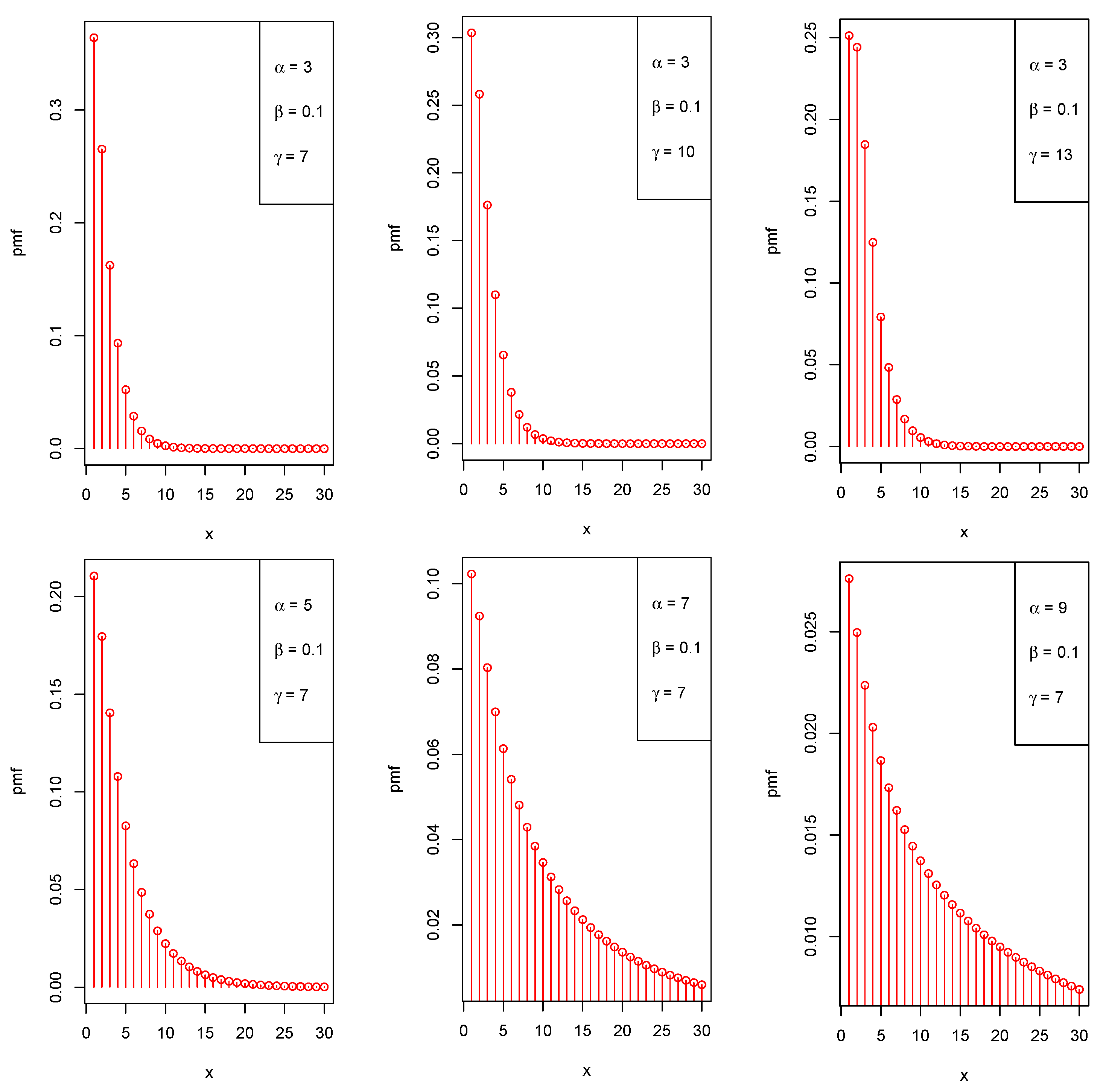
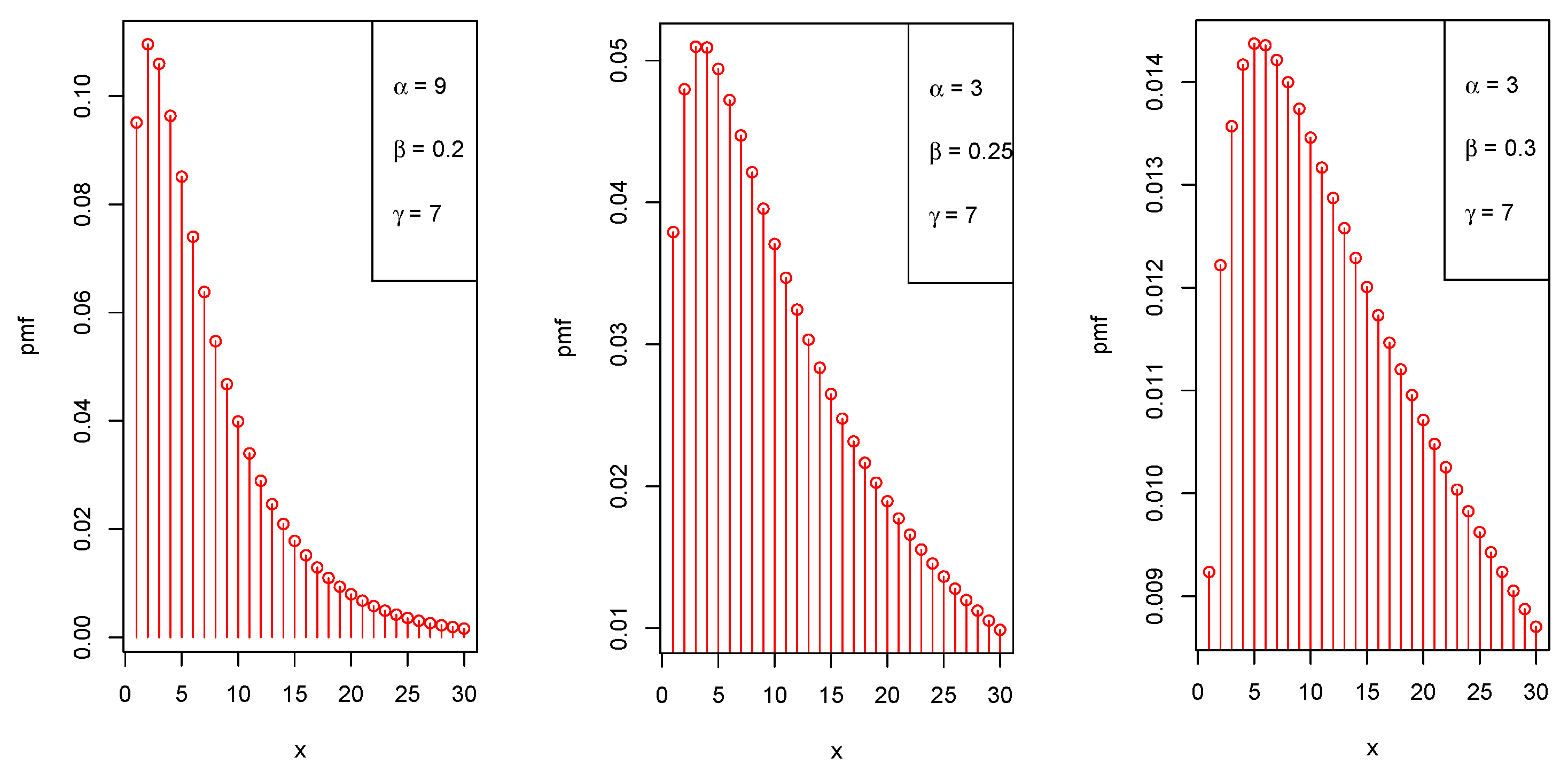
Now, Figure 1 portrays the graphical representation of the LZTBD for different parameter values of α , β , and γ .
The hazard rate function (hrf) of the LZTBD is obtained by substituting the pmf in the following equation:
f x = P ( X = x | X x ) = f ( x ) j = x f ( j ) , x = 1 , 2 , 3 ,
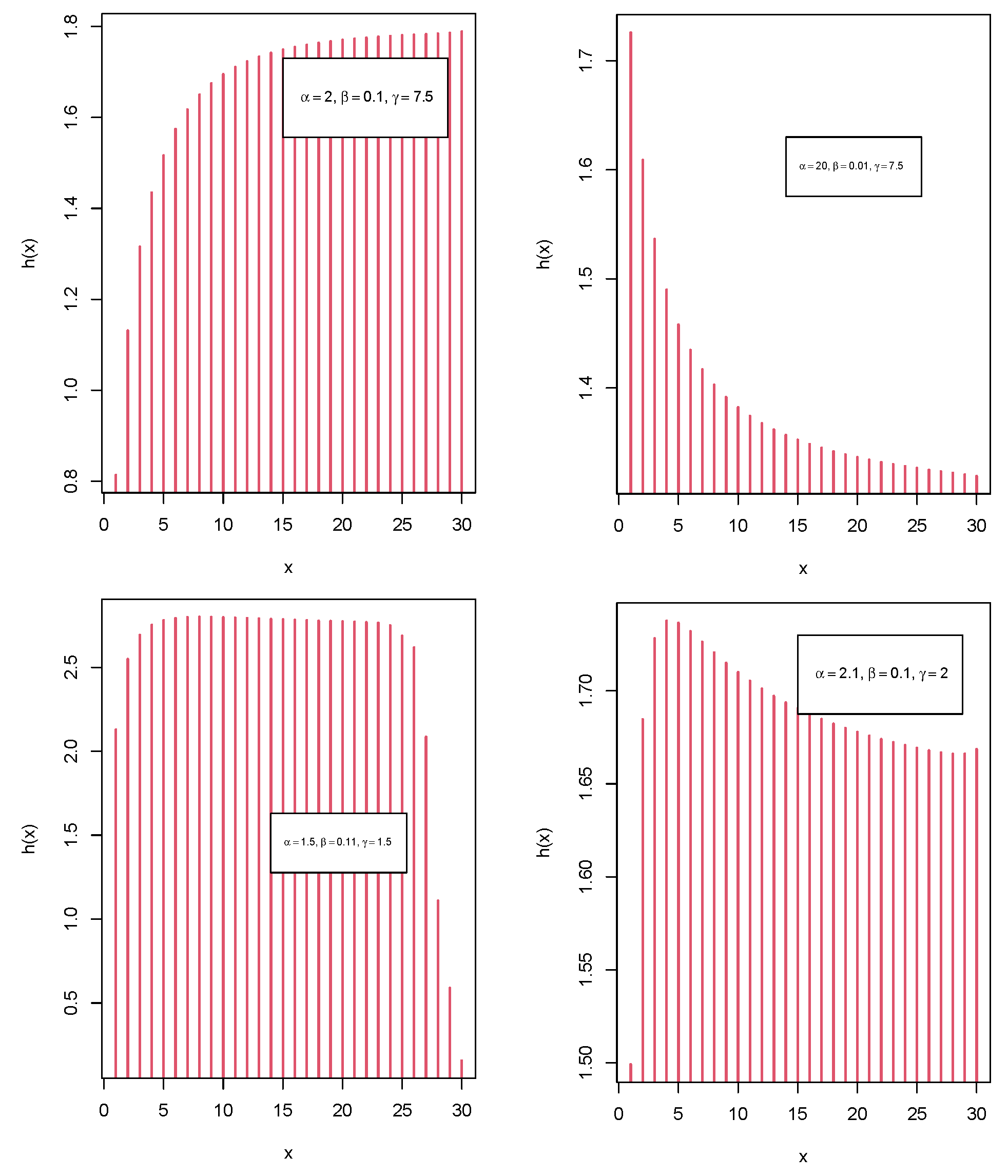
Following (6), it goes without saying that determining the closed form expression of the hrf is more difficult, although, in order to determine the shape of the hrf, we sketch its graph. Figure 2 demonstrates the following facts about the shapes of the hrf of the LZTBD, indicating that the LZTBD has all of the typical shapes, such as increasing, decreasing, and bathtub shapes for varying parameter values.
Furthermore, the choice of various specific functions for g 2 ( z ) will provide various members of DLF. In the following, we list some DLF distributions available in the literature.

3.1. Poisson-Binomial Distribution

If we take g 1 ( z ) = ( 1 β + β z ) α and g 2 ( z ) = e γ ( z 1 ) , based on (3), the pmf of the considered distribution is obtained as
f 1 ( x ) = D x ( 1 β + β z ) α x e γ ( z 1 ) | z = 0 x ! = ( 1 α β ) e γ γ x ( 1 β ) α x x ! 2 F 0 x , α x ; β γ ( 1 β ) , x = 0 , 1 , 2 , 3 ,
where 2 F 0 is the hypergeometric function. Since their pmfs coincide, the corresponding distribution is identified as the Poisson-binomial distribution (see [23]).

3.2. Weighted Consul Distribution

If we take g 1 ( z ) = ( 1 β + β z ) α and g 2 ( z ) = z , based on (3), the pmf of the considered distribution can be derived as
f 2 ( x ) = ( 1 α β ) D x ( 1 β + β z ) α x z | z = 0 x ! = ( 1 α β ) α x x 1 β x 1 ( 1 β ) α x x + 1 , x = 1 , 2 , 3 ,
which is the pmf of the weighted Consul distribution (see [23]).

3.3. Weighted Delta Binomial Distribution

If we take g 1 ( z ) = ( 1 β + β z ) α and g 2 ( z ) = z γ , based on (3), the pmf of the considered distribution is obtained as
f 3 ( x ) = ( 1 α β ) D x ( 1 β + β z ) α x z γ | z = 0 x ! = ( 1 α β ) α x x γ β x γ ( 1 β ) α x x + γ , x = γ , γ + 1 , γ + 2 ,
which corresponds to the pmf of the weighted delta binomial distribution (see [23]).

3.4. Linear Function Binomial Distribution

If we take g 1 ( z ) = ( 1 β + β z ) α and g 2 ( z ) = ( 1 β + β z ) γ , based on (3), the pmf of the considered distribution can be derived as
f 4 ( x ) = ( 1 α β ) D x ( 1 β + β z ) α x ( 1 β + β z ) γ | z = 0 x ! = ( 1 α β ) γ + α x x β x ( 1 β ) γ + α x x , x = 0 , 1 , 2 ,
which is the pmf of the linear function binomial distribution (see [23]).
Proposition 2.
Let X be an rv following the LZTBD. Then, the median of X is defined by the smaller integer m greater or equal to 1 such that
x = 1 m γ + α x x α x x β x ( 1 β ) α x x 1 ( 1 β ) γ 2 ( 1 β ) γ ( 1 α β ) .
Proof. 
By the definition, m is the smallest integer in the support of the rv, i.e., 1 , 2 , , such that P ( X m ) 1 2 , which is equivalent to the desired result. □
Proposition 3.
Let X be a rv following the LZTBD. Then, the mode of X, denoted by xm, exists in 1 , 2 , and lies in the case:
η ( x m + 1 ) η ( x m ) 1 β ( 1 β ) α 1 η ( x m ) η ( x m 1 ) ,
where η ( x m ) = γ + α x m x m α x m x m .
Proof. 
We must find the integer x = x m for which f ( x ) has the greatest value. That is, we aim to solve f ( x ) f ( x 1 ) and f ( x ) f ( x + 1 ) . First, note that f ( x ) can also be written as
f ( x ) = ( 1 α β ) β x ( 1 β ) γ + α x x η ( x ) 1 ( 1 β ) γ ,
where η ( x ) = γ + α x x α x x .
Obviously, f ( x ) f ( x 1 ) implies that
η ( x ) η ( x 1 ) 1 β ( 1 β ) α 1 .
Additionally, f ( x ) f ( x + 1 ) implies that
η ( x + 1 ) η ( x ) 1 β ( 1 β ) α 1 .
By combining (9) and (10), we obtain (8). □
Proposition 4.
The pgf of an rv X following the LZTBD is expressed as
Ψ ( u ) = E ( u X ) = ( 1 α β ) { ( 1 β + β z ) γ ( 1 β ) γ } ( 1 ( 1 β ) γ ) 1 z α β 1 β + β z ,
where z = u ( 1 β + β z ) α .
Proof. 
Using (4), the pgf of the LZTBD is of the following form:
Ψ ( u ) = ( 1 g 1 ( 1 ) ) g 2 ( z ) 1 z g 1 ( z ) g 1 ( z ) = ( 1 α β ) { ( 1 β + β z ) γ ( 1 β ) γ } ( 1 ( 1 β ) γ ) 1 z α β 1 β + β z .
Thus, the proof is complete. □
Corollary 1.
The moment generating function (mgf) of an rv X following the LZTBD is obtained by putting z = e s and u = e k in (11). That is,
M ( k ) = E ( e k X ) = ( 1 α β ) { ( 1 β + β e s ) γ ( 1 β ) γ } ( 1 ( 1 β ) γ ) 1 α β e s 1 β + β e s ,
where s = k + α log ( 1 β + β e s ) .
Corollary 2.
The cumulant generating function (cgf) of an rv X following the LZTBD becomes
C ( k ) = log M ( k ) = log ( 1 α β ) { ( 1 β + β e k ) γ ( 1 β ) γ } ( 1 ( 1 β ) γ ) 1 α β e s 1 β + β e s ,
where s = k + α log ( 1 β + β e s ) .
Proposition 5.
Let X 1 , X 2 , , X n be n independently and identically distributed (iid) rvs following the LZTBD( α , β , γ ). Then, the distribution of the random sum variable V = i = 1 n X i has the following pgf:
Ψ 1 ( u ) = ( 1 α β ) n { ( 1 β + β z ) γ ( 1 β ) γ } n ( 1 ( 1 β ) γ ) n 1 z α β 1 β + β z n ,
where z = u ( 1 β + β z ) α .
Proof. 
Based on the pgf of the LZTBD given in (11), the pgf of the rv V becomes
Ψ 1 ( u ) = E ( u V ) = E ( u X 1 + X 2 + + X n ) = i = 1 n E ( u X i ) = i = 1 n Ψ ( u ) = [ Ψ ( u ) ] n = ( 1 α β ) n { ( 1 β + β z ) γ ( 1 β ) γ } n ( 1 ( 1 β ) γ ) n 1 z α β 1 β + β z n .
This completes the proof. □
Proposition 6.
For any integer r 1 , the r t h factorial moment of an rv X following the LZTBD( α , β , γ ) is given by
μ [ r ] = E X ( X 1 ) ( X 2 ) ( X r + 1 ) = { 1 ( 1 β ) γ 1 D r 1 β + β z ) γ + α β i = 1 r ( r i + 1 ) μ [ r i ] D i u ( 1 β + β z ) α 1 1 α β } | u = z = 1 ,
where z = u ( 1 β + β z ) α .
Proof. 
By definition, the r t h factorial moment of the LZTBD( α , β , γ ) is obtained by successively differentiating Ψ ( u ) given in (11) r times with respect to (wrt) u and by putting u = z = 1 . First, note that
( 1 u g 1 ( z ) ) Ψ ( u ) = ( 1 g 1 ( 1 ) ) g 2 ( z ) .
Taking the first derivative wrt u on both sides, we obtain
Ψ ( u ) D 1 ( 1 u g 1 ( z ) ) + Ψ ( u ) ( 1 u g 1 ( z ) ) = ( 1 g 1 ( 1 ) ) D 1 g 2 ( z ) .
Taking the second derivative of the above equation wrt u on both sides, we obtain
Ψ ( u ) D 2 ( 1 u g 1 ( z ) ) + 2 D 1 ( 1 u g 1 ( z ) ) Ψ ( u ) + ( 1 u g 1 ( z ) ) Ψ ( u ) = ( 1 g 1 ( 1 ) ) D 2 g 2 ( z ) .
Proceeding in a similar manner, the r t h derivative is of the following form:
D r Ψ ( u ) = ( 1 g 1 ( 1 ) ) D r g 2 ( z ) i = 1 r ( r i + 1 ) D i ( 1 u g 1 ( z ) ) D r i Ψ ( u ) 1 u g 1 ( z ) .
Substitute g 1 ( z ) = ( 1 β + β z ) α , g 2 ( z ) = ( 1 β + β z ) γ ( 1 β ) γ 1 ( 1 β ) γ and z = u = 1 , in (15), we obtain (14). □
Proposition 7.
The mean (μ) and variance ( σ 2 ) for the LZTBD are of the following forms, respectively,
μ = γ β ( 1 ( 1 β ) γ ) ( 1 α β ) + α β ( 1 β ) ( 1 α β ) 2
and
σ 2 = α β + ( α 2 3 α ) β 2 + ( 2 α α 2 ) β 3 + 2 α 3 β 4 ( 1 α β ) 4 + γ 2 β 2 + γ β ( 1 β ) γ 2 α β 3 ( 1 ( 1 β ) γ ) ( 1 α β ) 3 γ 2 β 2 ( 1 ( 1 β ) γ ) 2 ( 1 α β ) 2 .
Proof. 
Using (14), we obtain
μ = E ( X ) = g 2 ( 1 ) ( 1 g 1 ( 1 ) ) + g 1 ( 1 ) + g 1 ( 1 ) ( g 1 ( 1 ) ) 2 ( 1 g 1 ( 1 ) ) 2 = γ β ( 1 ( 1 β ) γ ) ( 1 α β ) + α β ( 1 β ) ( 1 α β ) 2 .
On the other hand, we have
σ 2 = E X ( X 1 ) + E X E X 2 = g 2 ( 1 ) + g 2 ( 1 ) ( g 2 ( 1 ) ) 2 ( 1 g 1 ( 1 ) ) 2 + ( 1 + g 2 ( 1 ) ) g 1 ( 1 ) + g 1 ( 1 ) ( g 1 ( 1 ) ) 2 ) ( 1 g 1 ( 1 ) ) 3 + g 1 ( 1 ) + g 1 ( 1 ) g 1 ( 1 ) + 2 g 1 ( 1 ) ( 1 g 1 ( 1 ) ) 3 + 2 ( g 1 ( 1 ) ) 2 ( 1 g 1 ( 1 ) ) 4 = α β + ( α 2 3 α ) β 2 + ( 2 α α 2 ) β 3 + 2 α 3 β 4 ( 1 α β ) 4 + γ 2 β 2 + γ β ( 1 β ) γ 2 α β 3 ( 1 ( 1 β ) γ ) ( 1 α β ) 3 γ 2 β 2 ( 1 ( 1 β ) γ ) 2 ( 1 α β ) 2 .
The desired expressions are obtained. □
A normalized measure of dispersion can be obtained by utilizing the variance-to-mean relationship. This measure is the well-known index of dispersion (IOD). The next result expressed it for the LZTBD, among others.
Proposition 8.
The IOD and coefficient of variation (CV) for the LZTBD are given as, respectively,
IOD = α β + ( α 2 3 α ) β 2 + ( 2 α α 2 ) β 3 + 2 α 3 β 4 ( 1 α β ) 4 + γ 2 β 2 + γ β ( 1 β ) γ 2 α β 3 ( 1 ( 1 β ) γ ) ( 1 α β ) 3 γ 2 β 2 ( 1 ( 1 β ) γ ) 2 ( 1 α β ) 2 γ β ( 1 ( 1 β ) γ ) ( 1 α β ) + α β ( 1 β ) ( 1 α β ) 2
and
CV = α β + ( α 2 3 α ) β 2 + ( 2 α α 2 ) β 3 + 2 α 3 β 4 ( 1 α β ) 4 + γ 2 β 2 + γ β ( 1 β ) γ 2 α β 3 ( 1 ( 1 β ) γ ) ( 1 α β ) 3 γ 2 β 2 ( 1 ( 1 β ) γ ) 2 ( 1 α β ) 2 γ β ( 1 ( 1 β ) γ ) ( 1 α β ) + α β ( 1 β ) ( 1 α β ) 2 .
Proof. 
We have
IOD = σ 2 μ = α β + ( α 2 3 α ) β 2 + ( 2 α α 2 ) β 3 + 2 α 3 β 4 ( 1 α β ) 4 + γ 2 β 2 + γ β ( 1 β ) γ 2 α β 3 ( 1 ( 1 β ) γ ) ( 1 α β ) 3 γ 2 β 2 ( 1 ( 1 β ) γ ) 2 ( 1 α β ) 2 γ β ( 1 ( 1 β ) γ ) ( 1 α β ) + α β ( 1 β ) ( 1 α β ) 2 .
Analogously, the CV is given by
CV = σ 2 μ = α β + ( α 2 3 α ) β 2 + ( 2 α α 2 ) β 3 + 2 α 3 β 4 ( 1 α β ) 4 + γ 2 β 2 + γ β ( 1 β ) γ 2 α β 3 ( 1 ( 1 β ) γ ) ( 1 α β ) 3 γ 2 β 2 ( 1 ( 1 β ) γ ) 2 ( 1 α β ) 2 γ β ( 1 ( 1 β ) γ ) ( 1 α β ) + α β ( 1 β ) ( 1 α β ) 2 .
A probabilistic model’s asymmetry degree and flatness are commonly assessed by their skewness and kurtosis coefficients, respectively. The third central moment, normalized by the variance raised to the power of 3 / 2 , can be used to calculate the first, whereas the fourth central moment divided by the square of the variance can be used to calculate the second. Mean, variance, CV, IOD, skewness, and kurtosis for selected values of parameters of the LZTBD( α , β , γ ) are summarized in Table 1. From this table, it is evident that the LZTBD possesses both over-dispersion (IOD > 1 ) and under-dispersion (IOD < 1 ) for varying parameter values. It is also noted that the LZTBD is mainly right-skewed, and has several kurtosis levels.

4. Identifiability

Finite mixture models have received a lot of attention in recent years in real contexts. In astronomy, biology, genetics, medicine, psychiatry, marketing, and other fields, mixture models are widely utilized (see [24]). We derive finite mixtures of the LZTBD( α , β , γ ) in this section. This mixed model may be appropriate in the context of future initiatives.
Let Y be a discrete rv with the pmf h ( y ) = i = 1 g l i h i ( y ) , where i = 1 , 2 , g , l i > 0 such that i = 1 g l i = 1 , h i ( y ) 0 and y h i ( y ) = 1 . Then, we state that Y has a mixture distribution and h ( y ) is a finite mixture of distributions. The constants l 1 , l 2 , , l g are known as mixing weights and h 1 ( y ) , h 2 ( y ) , , h g ( y ) , the components of the mixture. We denote as Θ the collection of all distinct parameters in the components.
Let Σ = { U ( y ; θ i ) : θ i Θ } be the class of pmf’s from which mixtures are to be formed. Then, the class of finite mixtures of Σ with the appropriate class of pmf’s is Δ ^ = { Δ ( y ) : Δ ( y ) = i = 1 g l i U ( y ; θ i ) , l i > 0 , U ( y ; θ i ) Σ , i = 1 , 2 , g } . So that Δ ^ is the convex hull of Σ .
Definition 1.
An intege-valued rv Y is said to have a g component mixture of the LZTBDs if it has the pmf h ( y ) = P ( Y = y ) of the following form:
h ( y ) = i = 1 g l i h i ( y ) ,
where 0 l i 1 , for each i = 1 , 2 , 3 , g , i = 1 g l i = 1 ,
h i ( y ) = ( 1 α i β i ) [ γ i + α i y y α i y y ] β i y ( 1 β i ) γ i + α i y y ( 1 ( 1 β i ) γ i ) , y = 1 , 2 , ,
with γ i > 0 , 0 α i < β i 1 and 0 < β i < 1 for each i = 1 , 2 , , g .
A distribution with pmf given in (20) is called the Lagrangian zero-truncated binomial mixture distribution with g components (LZTBMDg).
The following theorem from [25] is adopted to construct the identifiability conditions of the finite mixture model.
Theorem 1.
A necessary and sufficient condition for Δ ^ to be identifiable is that Δ should be linearly independent over the field of real numbers.
Proof. 
The proof is stated in [25], hence, it is not included here. □
Next, applying Theorem 1, we outline the LZTBMDg’s identifiability requirements.
Theorem 2.
The identifiability conditions for the LZTBMDg with the pmf h ( y ) as given in (20) are α i α j , β i β j , and γ i γ j for i , j { 1 , 2 , , g } , such that i j .
Proof. 
For the first step, take g = 2 and consider the following equation:
b 1 F 1 ( y ) + b 2 F 2 ( y ) = 0 ,
where b 1 and b 2 are any two arbitrary real numbers, F 1 ( y ) = j = 1 y h ( j ) and F 2 ( y ) = j = 1 y ϕ ( j ) for y = 1 , 2 , , in which ϕ ( j ) is obtained from h ( j ) by replacing α j by τ j , β j by δ j and γ j by ω j .
Assume that for each i = 1 , 2 and α i τ i , β i δ i and γ i ω i . Thus, for l 1 = l , we have
F 1 ( y ) = l j = 1 y ( 1 α 1 β 1 ) γ 1 + α 1 j j α 1 j j β 1 j ( 1 β 1 ) γ 1 + α 1 j j 1 ( 1 β 1 ) γ 1 + ( 1 l ) j = 1 y ( 1 α 2 β 2 ) γ 2 + α 2 j j α 2 j j β 2 j ( 1 β 2 ) γ 2 + α 2 j j 1 ( 1 β 2 ) γ 2
and
F 2 ( y ) = l j = 1 y ( 1 τ 1 δ 1 ) ω 1 + τ 1 j j τ 1 j j δ 1 j ( 1 δ 1 ) ω 1 + τ 1 j j 1 ( 1 δ 1 ) ω 1 + ( 1 l ) j = 1 y ( 1 τ 2 δ 2 ) ω 2 + τ 2 j j τ 2 j j δ 2 j ( 1 δ 2 ) ω 2 + τ 2 j j 1 ( 1 δ 2 ) ω 2 .
Now, from (22)–(24), we obtain the following equations:
b 1 j = 1 y ( 1 α 1 β 1 ) γ 1 + α 1 j j α 1 j j β 1 j ( 1 β 1 ) γ 1 + α 1 j j 1 ( 1 β 1 ) γ 1 + b 2 j = 1 y ( 1 τ 1 δ 1 ) ω 1 + τ 1 j j τ 1 j j δ 1 j ( 1 δ 1 ) ω 1 + τ 1 j j 1 ( 1 δ 1 ) ω 1 = 0
and
b 1 j = 1 y ( 1 α 2 β 2 ) γ 2 + α 2 j j α 2 j j β 2 j ( 1 β 2 ) γ 2 + α 2 j j 1 ( 1 β 2 ) γ 2 + b 2 j = 1 y ( 1 τ 2 δ 2 ) ω 2 + τ 2 j j τ 2 j j δ 2 j ( 1 δ 2 ) ω 2 + τ 2 j j 1 ( 1 δ 2 ) ω 2 = 0 .
Solving (25) and (26), we obtain
b 1 j = 1 y ( 1 α 1 β 1 ) ( 1 τ 2 δ 2 ) ( β 1 δ 2 ) j ( 1 β 1 ) γ 1 + α 1 j j ( 1 δ 2 ) ω 2 + τ 2 j j [ γ 1 + α 1 j j α 1 j j ] [ ω 2 + τ 2 j j τ 2 j j ] ( 1 ( 1 β 1 ) γ 1 ) ( 1 ( 1 δ 2 ) ω 2 = b 1 j = 1 y ( 1 α 2 β 2 ) ( 1 τ 1 δ 1 ) ( β 2 δ 1 ) j ( 1 β 2 ) γ 2 + α 2 j j ( 1 δ 1 ) ω 1 + τ 1 j j [ γ 2 + α 2 j j α 2 j j ] [ ω 1 + τ 1 j j τ 1 j j ] ( 1 ( 1 β 2 ) γ 2 ) ( 1 ( 1 δ 1 ) ω 1 .
Hence, by (27), we have b 1 = 0 and thus, b 2 = 0 . Therefore, it may be inferred from Theorem 2 that F 1 ( y ) and F 2 ( y ) are linearly independent. Now that the argument may be applied to any positive integer g, the proof follows. □
Proposition 9.
The pgf of the LZTBMDg given in (20) is indicated as
Ψ ( u ) = i = 1 g ( 1 α i β i ) { ( 1 β i + β i z i ) γ i ( 1 β i ) γ i } ( 1 ( 1 β i ) γ i ) ( 1 z i α i β i 1 β i + β i z i ) ,
where z i = u ( 1 β i + β i z i ) α i .
Proof. 
The proof follows simply from Definition 1, given the pgf of the LZTBD mentioned in (11). □

5. Estimation of Parameters

In this section, we estimate the unknown parameters of the LZTBD by the ML estimation method.
It is worth mentioning that the model corresponding to the LZTBD ( α , β , γ ) is a tri-parametric model with parameters α , β , and γ . Let us have a random sample of size n from LZTBD and let the observed frequency be n x , x = 1 , 2 , , k , so that x = 1 k n x = n , where k is the largest of the observed value having non-zero frequencies. Then, the likelihood function is given by
L = x = 1 k ( 1 α β ) β x ( 1 β ) γ + α x x γ + α x x α x x ( 1 ( 1 β ) γ ) n x .
Therefore, the log-likelihood function is given by
L n = logL = n log ( 1 α β ) + n x ¯ log β + ( n γ + n x ¯ ( α 1 ) ) log ( 1 β ) n log ( 1 ( 1 β ) γ ) + x = 1 k n x log i = 0 x 1 ( γ + α x i ) i = 0 x 1 ( α x i ) x = 1 k n x log ( x ! ) ,
where x ¯ = 1 n x = 1 k x n x . The ML estimates (MLEs) are defined by maximizing L n wrt the parameters. Let us denote by α ^ , β ^ , and γ ^ the MLEs of α , β , and γ , respectively. On the computational side, the score vector is
S = L n α L n β L n γ T ,
where the partial derivatives of L n wrt the parameters are
L n α = n x ¯ log ( 1 β ) n β 1 α β + x = 1 k n x α i = 0 x 1 ( γ + α x i ) i = 0 x 1 ( α x i ) i = 0 x 1 ( γ + α x i ) i = 0 x 1 ( α x i ) ,
L n β = n x ¯ β n α ( 1 α β ) n γ + n ( α 1 ) x ¯ 1 β n γ ( 1 β ) γ 1 1 ( 1 β ) γ
and
L n γ = n log ( 1 β ) + n γ ( 1 β ) γ 1 1 ( 1 β ) γ + x = 1 k n x γ i = 0 x 1 ( γ + α x i ) i = 0 x 1 ( γ + α x i ) i = 0 x 1 ( α x i ) .
The MLEs can then be found by setting the score vector to zero, i.e., S = 0 , and solving them concurrently. These equations cannot be solved analytically, and the R statistical software can be used to solve them numerically by means of iterative techniques such as the Newton–Raphson algorithm.

6. Likelihood Ratio Test

In this section, we test the significance of an additional parameter included in the LZTBD using the generalized likelihood ratio test (GLRT) (see [26]).
More precisely, to test the significance of the parameter α of the LZTBD ( α , β , γ ) , here, we consider the GLRT procedure. The null hypothesis H 0 : X follows the ZTBD” against the alternative hypothesis H 1 : X follows the LZTBD”. Here, the test statistic is given by
2 log λ * = 2 L n ( Θ ^ ) L n ( Θ ^ * ) ,
where Θ ^ is the vector of MLEs of Θ = ( α , β , γ ) with no constraints, and Θ ^ * is the MLEs of Θ under H 0 .

7. Simulation

We perform a simulation study by generating observations employing the R software to examine the asymptotic behavior of the MLEs of the parameters of the LZTBD. Here, we apply the inverse transformation method to simulate a LZTBD random sample (see [27]). The algorithm is as follows:
Step 1:
Generate a random number from the uniform U ( 0 , 1 ) distribution.
Step 2:
i = 1 , P = ( 1 α β ) β γ ( 1 β ) γ + α 1 , F = P .
Step 3:
If U < F , set X = i and stop.
Step 4:
P = P × β ( 1 β ) α 1 ( γ + α i ) γ + α ( i + 1 ) i + 1 ( γ + α ( i + 1 ) ) γ + α i i , F = F + P , i = i + 1 .
Step 5:
Go to Step 3.
Conceptually, P is the probability that X = i , and F is the probability that X is less than or equal to i.
Additionally, indices such as MLEs, absolute biases, and mean squared errors (MSEs) are calculated using the following equations:
  • Average value of MLEs: MLE( a ^ ) = 1 N i = 1 N a ^ i .
  • Absolute average bias: Bias( a ^ ) = 1 N i = 1 N | a ^ i a | .
  • MSE: MSE( a ^ ) = 1 N i = 1 N ( a ^ i a ) 2 .
Here, a = α or β or γ , and the index i represents the i t h generated sample. The simulation takes into account sample sizes of n = 15, 50, 175, 500, and 1000 for two different sets of parameter values of the LZTBD. We repeat the process N = 1000 times and report the estimates and MSEs in Table 2. From this table, one can infer that the estimates are quite stable and, more precisely, close to the true parameter values for these sample sizes. A decreasing trend is being observed in the absolute average bias and MSEs as we increase the sample size. Hence, the performance of the ML estimation is quite consistent and reliable.
8. Applications and Empirical Study

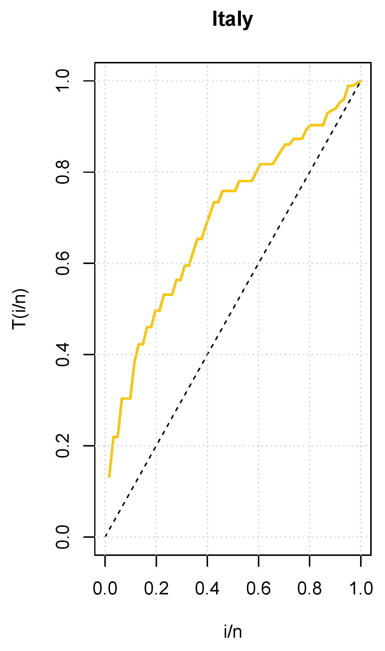
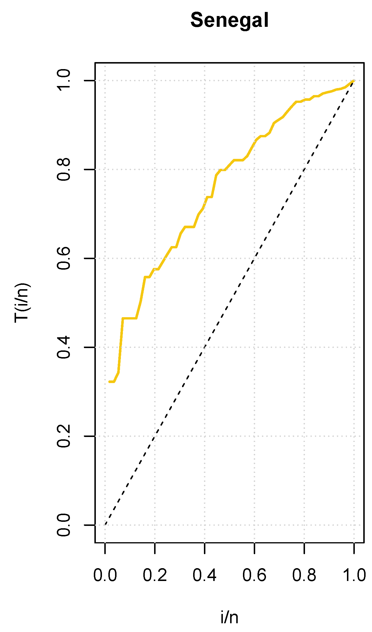
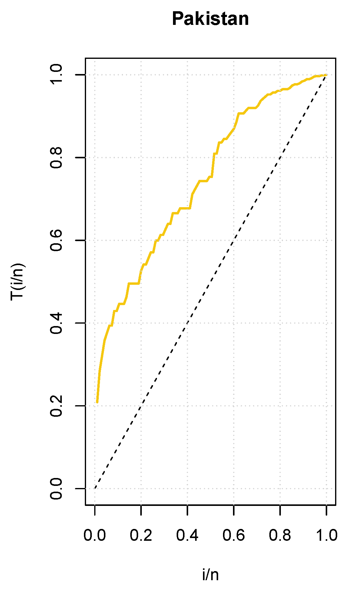
The aim of this section is to show the empirical importance of the LZTBD. We employ six genuine datasets to apply the superiority of the LZTBD fit to the more notable fields of COVID-19 with different nations, including Italy, Senegal, Pakistan, Saudi Arabia, Belgium, and Ethiopia. The graphical method used to determine the hrf of the data set is based on the Total Time on Test (TTT). Convex, concave, convex-then-concave, and concave-then-convex empirical TTT plots correspond to decreasing, increasing, bathtub shape, and upside-down bathtub shape for the corresponding hrf, respectively (see [28]). We employ the statistical software R to evaluate these datasets numerically. To show the possible benefit of the LZTBD, the distributions below are depicted:
  • ZTBD with parameters β and γ , which has the following pmf:
    f 5 ( x ) = γ x β x ( 1 β ) γ x 1 ( 1 β ) x , x = 1 , 2 , 3
  • Zero-truncated generalized binomial distribution (ZTGBD) with parameters α , β , and γ with the following pmf:
    f 6 ( x ) = γ γ + α x γ + α x x β x ( 1 β ) γ + α x x 1 ( 1 β ) γ , x = 1 , 2 , 3
  • Zero-truncated discrete two parameter Poisson–Lindley distribution (ZTDTPPLD) with parameters γ and β (see [29]), which have the following pmf:
    f 7 ( x ) = γ 2 γ 2 + 2 γ β + γ + β β x + γ + β + 1 ( γ + 1 ) x , x = 1 , 2 , 3
  • Zero-truncated Poisson–Lindley distribution (ZTPLD) with parameters α (see [30]), which has the following pmf:
    f 8 ( x ) = α 2 ( x + α + 2 ) ( α 2 + 3 α + 1 ) ( α + 1 ) x , x = 1 , 2 , 3 ,
  • Intervened generalized Poisson distribution (IGPD) with parameters α , β , and γ (see [31]), which has the following pmf:
    f 9 ( x ) = α ( 1 + γ ) ( 1 + γ ) α + β x x 1 γ γ α + β x x 1 e α γ + β x e α 1 x ! , x = 1 , 2 , 3

8.1. COVID-19 Data Set from Italy

Italy’s 61-day COVID-19 data collection, conducted from 13 June to 12 August 2021, is accessible in [11]. Daily newly reported cases are included in this data collection. The descriptive measures of the real data set, which include sample size (n), minimum (min), first quartile ( Q 1 ), median ( M d ), third quartile ( Q 3 ), maximum (max), and inter-quartile range ( I Q R ) are given in Table 3.
In addition, Figure 3 shows an empirical TTT plot of the data, from which we deduce an increasing hrf.
We compare the competitive distributions to the LZTBD using the statistical techniques provided, namely, the negative log-likelihood ( log L ), Akaike information criterion (AIC), Bayesian information criterion (BIC), and χ 2 statistic. Table 4 displays the corresponding MLEs, model adequacy measures, and χ 2 values. The LZTBD has lower model adequacy measures and χ 2 values than the other distributions studied, as shown in Table 4. As a result, the suggested model is the most appropriate for modeling the given COVID-19 data. It is interesting to note that the empirical mean, variance, and IOD of this COVID-19 data set are 22.6229, 160.3388, and 7.0874, respectively, and the theoretical values for the mean, variance, and IOD measures of the LZTBD are 21.6234, 160.3248, and 7.4144, respectively. Thus, the empirical and theoretical means are almost the same, and the empirical and theoretical variances and IOD values are close to each other.
In the case of GLRT, the calculated value based on the test statistic (29) is 2 ( 234.5071 + 485.9380 ) = 251.4309 (p-value = 0.0001 ). As a result, at any level greater than 0.0001, the null hypothesis is rejected in favor of the alternative hypothesis. Hence, we conclude that the additional parameter α in the LZTBD is significant in light of the test procedure outlined in Section 6.

8.2. COVID-19 Data Set from Senegal

The LZTBD is fitted to another set of data for the COVID-19 in Senegal for 56 days of infection, which was recorded from 29 March 2021 to 23 May 2021. These data, which show the daily incidence of COVID-19 cases, were gathered by the World Health Organization (WHO) and are accessible at http://covid19.who.int/data, (accessed on 24 August 2022). Table 5 includes some information as well as descriptive statistics for these data.
In addition, Figure 4 shows an empirical TTT plot of the data from which an increasing hrf is revealed.
We compare the competitive distributions to the suggested distribution using the statistical techniques provided, specifically, the log L , AIC, BIC, and χ 2 values. Table 6 displays the corresponding MLEs, model adequacy measures, and χ 2 values of the LZTBD. The LZTBD’s model adequacy measures and χ 2 values are less than those of the other examined models. As a result, the suggested model is the most appropriate for modeling the COVID-19 data from Senegal. It is worth noting that the empirical mean, variance, and IOD of these COVID-19 datasets are 46.54, 394.326, and 8.47, respectively, and the theoretical values for the mean, variance, and IOD measures of the LZTBD are 46.4, 394.324, and 8.49, respectively. Thus, the empirical and theoretical means are almost the same, and the empirical and theoretical variances and IOD values are very close to each other.
In the case of GLRT, the calculated value based on the test statistic (29) is 2 ( 244.0212 + 584.8307 ) = 340.8095 (p-value = 0.0004 ). As a result, at any level greater than 0.0004, the null hypothesis is rejected in favor of the alternative hypothesis. Hence, we conclude that the additional parameter α in the LZTBD is significant in light of the test procedure outlined in Section 6.

8.3. COVID-19 Data Set from Pakistan

The LZTBD is fitted to another set of data for the COVID-19 in Pakistan for 95 days of infection, which was recorded from 23 May 2021 to 25 August 2021. These data, which are available at http://covid19.who.int/data, (accessed on 24 August 2022), were acquired by the WHO and show the daily incidence of COVID-19 cases. Table 7 contains some information and descriptive statistics for these data.
In addition, Figure 5 shows an empirical TTT plot of the data, showing an increasing hrf.
Using the statistical methods offered, specifically the log L , AIC, BIC, and χ 2 values, we compare the competing distributions to the suggested distribution. Table 8 displays the corresponding MLEs, model adequacy measures, and χ 2 values of the LZTBD. The LZTBD’s model adequacy measures and χ 2 values are less than those of the other examined models. The suggested model is, therefore, the most suitable one to model the COVID-19 data from Pakistan. In addition, let us mention that the empirical mean, variance, and IOD of this COVID-19 dataset are 52.6842, 538.5801, and 10.2228, respectively, and the theoretical values for the mean, variance, and IOD measures of the LZTBD are 52.6704, 538.5509, and 10.2249, respectively. We thus observe that the empirical and theoretical means are almost equal, and the empirical and theoretical variances and IOD values are very close to each other.
In the case of GLRT, the calculated value based on the test statistic (29) is 2 ( 431.4451 + 1313.275 ) = 881.8299 (p-value = 0.0001 ). As a result, at any level greater than 0.0001, the null hypothesis is rejected in favor of the alternative hypothesis. Hence, we conclude that the additional parameter α in the LZTBD is significant in light of the test procedure outlined in Section 6.

8.4. COVID-19 Data Set from Saudi Arabia

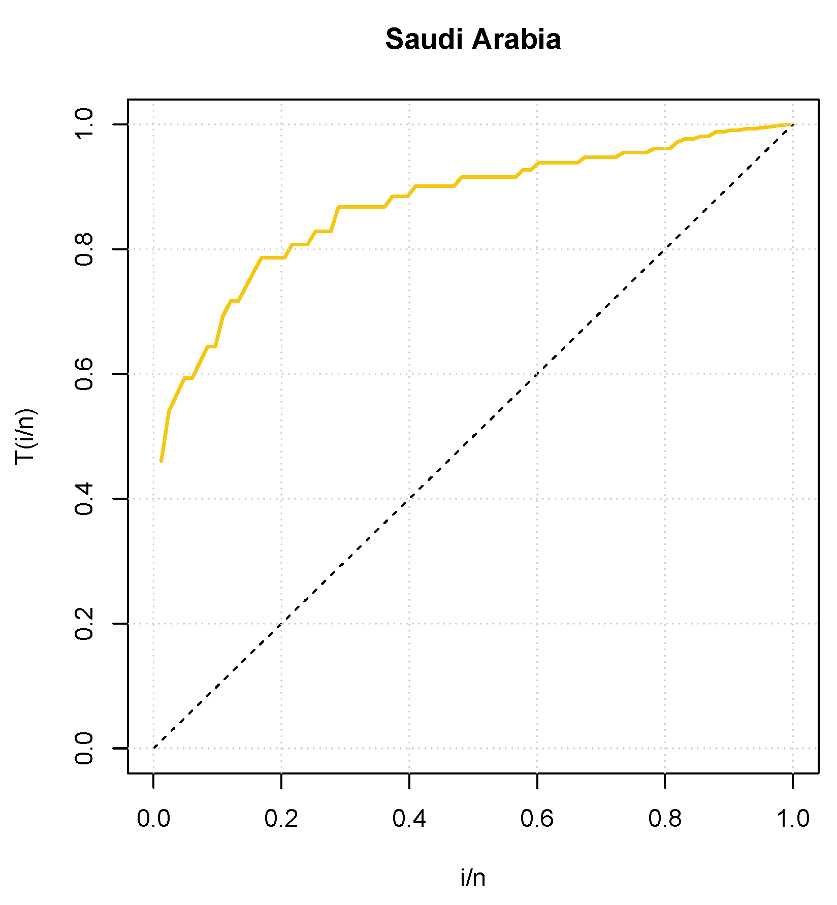
The LZTBD is fitted to another set of data of COVID-19 mortality numbers in Saudi Arabia for 83 days of infection, which was recorded from 30 May to 20 August 2020. The WHO gathered these data, which represent the number of deaths per day, and they are available at http://covid19.who.int/data, (accessed on 24 August 2022). Table 9 contains some information and descriptive statistics for these data.
In addition, Figure 6 shows an empirical TTT plot of the data and it shows an increasing hrf.
We compare the competitive distributions to the suggested distribution using the statistical techniques provided, specifically, the log L , AIC, BIC, and χ 2 values. Table 10 displays the corresponding MLEs, model adequacy measures, and χ 2 values of the LZTBD. The LZTBD’s model adequacy measures and χ 2 values are less than those of the other examined models. For modeling the COVID-19 data from Saudi Arabia, the suggested model is therefore the most suitable. Furthermore, the empirical mean, variance, and the IOD values of this COVID-19 dataset are 36.9277, 70.5313, and 1.9099, respectively, and the theoretical values for the mean, variance, and IOD measures of the LZTBD are 36.8724, 71.0567, and 1.9270, respectively. Hence, the empirical and theoretical means are almost the same, and the empirical and theoretical variances and IOD values are very close to each other.
In the case of GLRT, the calculated value based on the test statistic (29) is 2 ( 294.288 + 415.1392 ) = 120.8512 (p-value = 0.0002 ). As a result, at any level greater than 0.0002, the null hypothesis is rejected in favor of the alternative hypothesis. Hence, we conclude that the additional parameter α in the LZTBD is significant in light of the test procedure outlined in Section 6.

8.5. COVID-19 Data Set from Belgium

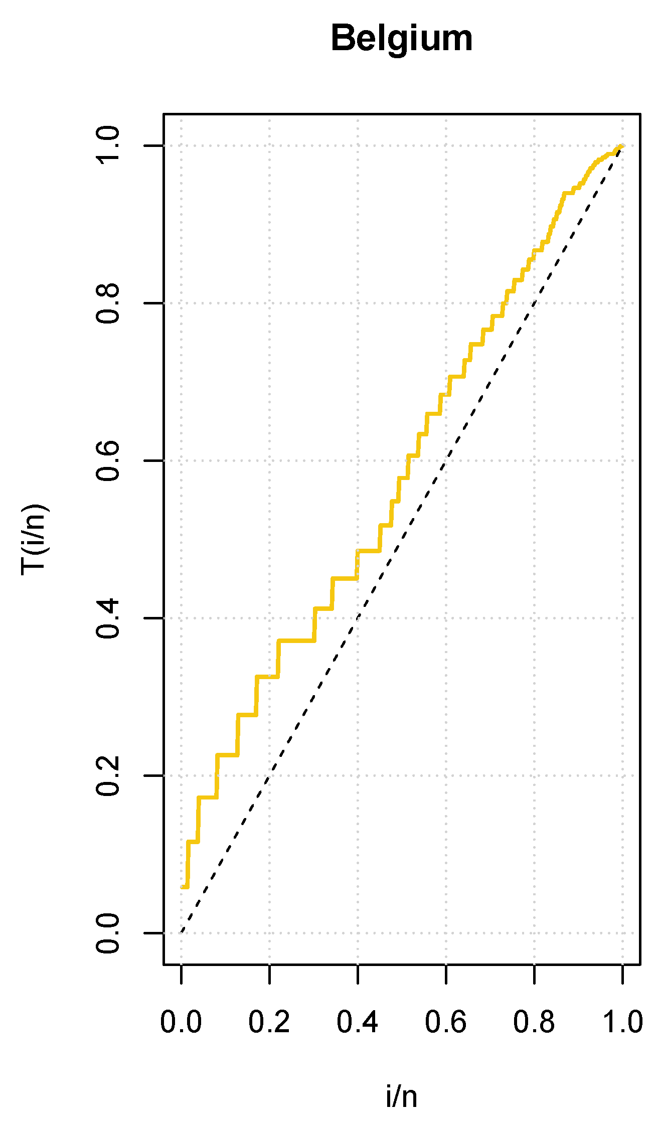
A different set of data on the COVID-19 infection in Belgium for 425 days (more than a year), which was recorded from 22 July 2021 to 19 September 2022, is fitted using the LZTBD. The WHO gathered these data, which represent the number of deaths per day, and are accessible at http://covid19.who.int/data, (accessed on 24 August 2022). Table 11 contains some information and descriptive statistics for these data.
In addition, Figure 7 shows an empirical TTT plot from which we can distinguish an increasing hrf.
We compare the competitive distributions to the suggested distribution using the statistical techniques provided, specifically, the log L , AIC, BIC, and χ 2 values. Table 12 displays the corresponding MLEs, model adequacy measures, and χ 2 values of the LZTBD. The LZTBD’s model adequacy measures and χ 2 values are less than those of the other examined models. As a result, the suggested model is the most appropriate for modeling the COVID-19 data from Belgium. It is worth noting that the empirical mean, variance, and IOD of this COVID-19 dataset are 17.122, 178.419, and 10.420, respectively, and the theoretical values for the mean, variance, and IOD measures of the LZTBD are 17.213, 178.412, and 10.365, respectively. Thus, the empirical and theoretical means are almost the same, and the empirical and theoretical variances and IOD values are very close to each other.
In the case of GLRT, the calculated value based on the test statistic (29) is 2 ( 1601.074 + 3825.833 ) = 2224.759 (p-value = 0.0012 ). As a result, at any level greater than 0.0012, the null hypothesis is rejected in favor of the alternative hypothesis. Hence, we conclude that the additional parameter α in the LZTBD is significant in light of the test procedure outlined in Section 6.

8.6. COVID-19 Data Set from Ethiopia

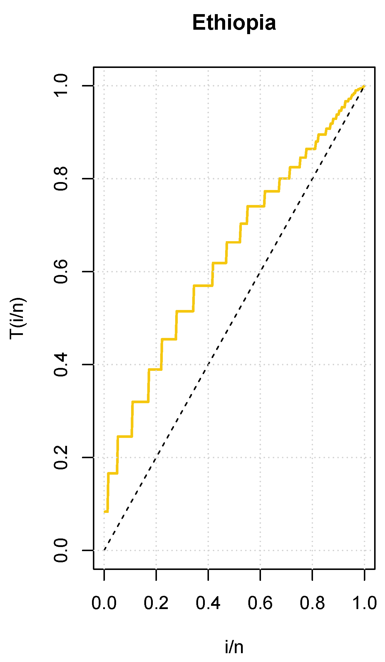
The LZTBD is fitted to another set of data on the COVID-19 infection in Ethiopia for 301 days, which was recorded from 25 August 2020 to 21 June 2021. The WHO collected these data, which represent the number of deaths per day, and are accessible at http://covid19.who.int/data, (accessed on 24 August 2022). Table 13 contains some information and descriptive statistics for these data.
As an additional result, Figure 8 shows an empirical TTT plot of the data, where an increasing hrf can be seen.
We use the statistical techniques provided to compare the competitive distributions to the suggested distribution, specifically, the log L , AIC, BIC, and χ 2 values. Table 14 displays the corresponding MLEs, model adequacy measures, and χ 2 values of the LZTBD. The LZTBD’s model adequacy measures and χ 2 values are less than those of the other examined models. The suggested model is therefore the most suitable one to model the Ethiopian COVID-19 data. In addition, it is found that the empirical mean, variance, and IOD of this COVID-19 dataset are 11.973, 67.00, and 5.5959, respectively, and the theoretical values for the mean, variance, and IOD measures of the LZTBD are 11.891, 67.02, and 5.6361, respectively. Thus, the empirical and theoretical means are almost equal, and the empirical and theoretical variances and IOD values are very close to each other.
In the case of GLRT, the calculated value based on the test statistic (29) is 2 ( 1003.902 + 1680.734 ) = 676.832 (p-value = 0.0002 ). As a result, at any level greater than 0.0002, the null hypothesis is rejected in favor of the alternative hypothesis. Hence, we conclude that the additional parameter α in the LZTBD is significant in light of the test procedure outlined in Section 6.

9. Conclusions

In this article, we used the Lagrange expansion to elaborate a new three-parameter distribution called the Lagrangian zero-truncated binomial distribution (LZTBD). It is worth noting that the proposed distribution is a generalized form of the well-known zero-truncated binomial distribution and the Lagrangian weighted Consul distribution. In particular, we paid close attention to the LZTBD. We investigated the shape properties of the probability mass and hazard functions. The expressions for the factorial moments, generating functions, mean, and median were derived. The identifiability of the LZTBD model was also proved. The LZTBD’s model parameters are estimated using the maximum likelihood estimation method. A study employing the simulation technique was also performed to show how well the maximum likelihood estimates are performing. Six actual datasets were used to validate the applicability and demonstrate that the LZTBD offers a superior fit to the competing models.

Author Contributions

Conceptualization, M.R.I., C.C., D.S.S., M.M. and R.M.; methodology, M.R.I., C.C., D.S.S., M.M. and R.M.; software, M.R.I., C.C., D.S.S., M.M. and R.M.; validation, M.R.I., C.C., D.S.S., M.M. and R.M.; formal analysis, M.R.I., C.C., D.S.S., M.M. and R.M.; investigation, M.R.I., C.C., D.S.S., M.M. and R.M.; resources, M.R.I., C.C., D.S.S., M.M. and R.M.; data curation, M.R.I., C.C., D.S.S., M.M. and R.M.; writing—original draft preparation, M.R.I., C.C., D.S.S., M.M. and R.M.; writing—review and editing, M.R.I., C.C., D.S.S., M.M. and R.M.; visualization, M.R.I., C.C., D.S.S., M.M. and R.M. All authors have read and agreed to the published version of the manuscript.

Funding

This research received no external funding.

Institutional Review Board Statement

Not applicable.

Informed Consent Statement

Not applicable.

Data Availability Statement

Not applicable.

Acknowledgments

The authors would also like to thank three reviewers for their thorough comments which led to improvement in the presentation of the manuscript.

Conflicts of Interest

The authors declare no conflict of interest.

References

  1. Finney, D.; Varley, G. An example of the truncated Poisson distribution. Biometrics 1955, 11, 387–394. [Google Scholar] [CrossRef]
  2. Creel, M.; Loomis, J. Theoretical and Empirical Advantages of Truncated Count Data Estimators for Analysis of Deer Hunting in California. Am. J. Agric. Econ. 1990, 72, 434–441. [Google Scholar] [CrossRef]
  3. Brass, W. Simplified methods of fitting the truncated negative binomial distribution. Biometrika 1959, 45, 59–68. [Google Scholar] [CrossRef]
  4. Lee, A.; Wang, K.; Yau, K.; Somerford, P. Truncated Negative Binomial Mixed Regression Modelling of Ischaemic Stroke Hospitalizations. Stat. Med. 2003, 22, 1129–1139. [Google Scholar] [CrossRef]
  5. Kennedy. Does Race Predict Stroke Readmission? An Analysis Using the Truncated Negative Binomial Model. J. Natl. Med. Assoc. 2005, 97, 699–713. [Google Scholar]
  6. Phange, A.; Loh, E. Zero Truncated Strict Arcsine Model. Int. J. Comput. Electr. Autom. Control. Inf. Eng. 2013, 7, 989–991. [Google Scholar]
  7. Zapata, Z.; Sedory, S.; Singh, S. Zero-truncated Binomial Distribution as a Randomization Device. Sociol. Methods Res. 2019, 51, 800–815. [Google Scholar] [CrossRef]
  8. Nesteurk, I. Statistics-based predictions of coronavirus epidemic spreading in mainland China. Innov. Biosyst. Bioeng. 2020, 4, 8–13. [Google Scholar] [CrossRef] [Green Version]
  9. El-Morshedy, M.; Altun, E.; Eliwa, M. A new statistical approach to model the counts of novel coronavirus cases. Math. Sci. 2021, 16, 37–50. [Google Scholar] [CrossRef]
  10. Ahsan-ul Haq, M.; Babar, A.; Hashmi, S.; Alghamdi, A.S.; Afify, A.Z. The Discrete Type-II Half-Logistic Exponential Distribution with Applications to COVID-19 Data. Pak. J. Stat. Oper. Res. 2021, 7, 921–932. [Google Scholar] [CrossRef]
  11. Almetwally, E.; Abdo, D.; Hafez, E.; Jawa, T.; Sayed-Ahmed, N.; Almongy, H. The new discrete distribution with application to COVID-19 Data. Results Phys. 2022, 32, 104987. [Google Scholar] [CrossRef] [PubMed]
  12. Lagrange, J.L. Mécanique Analytique; Jacques Gabay: Paris, France, 1788. [Google Scholar]
  13. Consul, P.C.; Shenton, L.R. Use of Lagrange expansion for generating generalized probability distributions. SIAM J. Appl. Math. 1972, 23, 239–248. [Google Scholar] [CrossRef]
  14. Consul, P.C.; Shenton, L.R. Some interesting properties of Lagrangian distributions. Commun. Stat. 1973, 2, 263–272. [Google Scholar] [CrossRef]
  15. Mohanty, S.G. On a generalized two-coin tossing problem. Biom. Z. 1966, 8, 266–272. [Google Scholar] [CrossRef]
  16. Consul, P.C.; Famoye, F. Lagrangian Katz family of distributions. Commun. Stat. Theory Methods 1996, 25, 415–434. [Google Scholar] [CrossRef]
  17. Berg, K.; Nowicki, K. Statistical inference for a class of modified power series distribution with applications to random mapping theory. J. Stat. Plan. Inference 1991, 28, 247–261. [Google Scholar] [CrossRef]
  18. Li, S.; Black, D.; Lee, C.; Famoye, F. Dependence Models Arising from the Lagrangian Probability Distributions. Commun. Stat.—Theory Methods 2010, 29, 1729–1742. [Google Scholar] [CrossRef]
  19. Innocenti, A.R.; Fox, O.; Chibbaro, S. A Lagrangian probability density-function model for collisional turbulent fluid-particle flows. J. Fluid Mech. 2019, 862, 449–489. [Google Scholar] [CrossRef] [Green Version]
  20. Jensen, J.L. Sur une identité d’ Abel et sur d’ autres formules analogues. Acta Math. 1902, 26, 307–318. [Google Scholar] [CrossRef]
  21. Riordan, J. Combinatorial Identities; John Wiley and Sons, Inc.: Newyork, NY, USA, 1968. [Google Scholar]
  22. Janardan, K.G.; Rao, B.R. Lagrangian distributions of second kind and weighted distributions. SIAM J. Appl. Math. 1983, 43, 302–313. [Google Scholar] [CrossRef]
  23. Consul, P.C.; Famoye, F. Lagrangian Probability Distributions; Birkhäuser: New York, NY, USA, 2006. [Google Scholar]
  24. McLachlan, G.; Peel, D. Finite Mixture Models; Wiley: Hoboken, NJ, USA, 2000. [Google Scholar]
  25. Titterington, D.M.; Smith, A.F.; Markov, U.E. Statistical Analysis of Finite Mixture Distributions; Wiley: Hoboken, NJ, USA, 1985. [Google Scholar]
  26. Rao, C.R. Minimum variance and the estimation of several parameters. Math. Proc. Camb. Philos. Soc. 1947, 43, 280–283. [Google Scholar] [CrossRef]
  27. Ross, S. Simulation, 5th ed.; Academic Press: Cambridge, MA, USA, 2013; pp. 5–38. [Google Scholar] [CrossRef]
  28. Aarset, M.V. How to identify a bathtub hazard rate. IEEE Trans. Reliab. 1987, 36, 106–108. [Google Scholar] [CrossRef]
  29. Shanker, R.; Shukla, K.K. Zero-Truncated Discrete Two-Parameter Poisson-Lindley Distribution with Applications. J. Inst. Sci. Technol. 2018, 22, 76–85. [Google Scholar] [CrossRef] [Green Version]
  30. Shanker, R.; Fesshaye, H.; Selvaraj, S.; Yemane, A. On zero-truncation of Poisson and Poisson-Lindley distributions and their applications. Biom. Biostat. Int. J. 2015, 2, 168–181. [Google Scholar] [CrossRef] [Green Version]
  31. Scollnik, D.M. On the Intervened Generalized Poisson Distribution. Commun. Stat.—Theory Methods 2006, 35, 953–963. [Google Scholar] [CrossRef]
Figure 1. Various shapes of the probability mass function (pmf) of the LZTBD for different values of the parameters.
Stats 05 00060 g001aStats 05 00060 g001b
Figure 2. Various shapes of the hazard rate function (hrf) of the LZTBD for different parameter values.
Stats 05 00060 g002
Figure 3. Total Time on Test (TTT) plot for the COVID-19 data set of Italy.
Stats 05 00060 g003
Figure 4. Total Time on Test (TTT) plot for the COVID-19 data set of Senegal.
Stats 05 00060 g004
Figure 5. Total Time on Test (TTT) plot for the COVID-19 data set of Pakistan.
Stats 05 00060 g005
Figure 6. Total Time on Test (TTT) plot for the COVID-19 data set of Saudi Arabia.
Stats 05 00060 g006
Figure 7. Total Time on Test (TTT) plot for the COVID-19 data set of Belgium.
Stats 05 00060 g007
Figure 8. Total Time on Test (TTT) plot for the COVID-19 data set of Ethiopia.
Stats 05 00060 g008
Table 1. Values of some moment measures of the LZTBD for various values of parameters α , β , and γ .
β γ α MeanVarianceCVIODSkewnessKurtosis
0.510.31.28020.15010.30260.11723.884714.6003
0.51.55550.44440.42850.28573.351110.1883
0.71.95261.22050.56570.62502.85616.9567
0.92.56193.45460.72541.34842.36694.3115
1.13.580210.76360.91633.00631.87122.1372
0.430.31.83230.73480.46780.40102.95687.4378
0.52.10071.13580.50730.54062.66125.7455
0.72.44991.84970.55510.75502.36504.2161
0.92.91893.21120.61391.10012.06242.8257
1.13.57506.02670.68661.68571.74921.5815
0.350.32.05741.06070.50050.51552.70045.9584
0.52.26651.41340.52420.62362.50574.9160
0.72.51781.92880.55150.76602.30893.9376
0.92.82452.70650.58240.95822.10843.0172
1.13.20563.92300.61781.22371.90272.1568
0.270.31.93891.00210.51630.51682.89347.2006
0.52.06711.21740.53370.58892.74716.3127
0.72.21131.49170.55230.67462.60455.5028
0.92.37451.84510.57200.77702.46394.7524
1.12.56012.30600.59310.90062.32424.0507
0.190.31.54330.58530.49570.37923.771813.9025
0.51.59630.66260.50990.41503.663813.0428
0.71.65260.75030.52410.45403.559012.2257
0.91.71230.85010.53840.49643.457211.4502
1.11.77570.96390.55280.54283.358010.7145
Table 2. The maximum likelihood estimates (MLEs) simulation results for the parameters α , β , and γ .
Parameter SetSample SizeParamtersEstimatesAbsolute BiasMSE
α = 0.5 ,   β = 0.16 ,   γ = 2.51 n = 15 α 4.30603.806020.4138
β 0.08380.07610.0138
γ 1.04521.46472.7145
n = 50 α 1.22450.72450.9985
β 0.13020.02970.0046
γ 1.36181.14812.0105
n = 175 α 0.69130.19130.2249
β 0.15820.00170.0019
γ 1.91220.59771.6952
n = 500 α 0.44760.05230.0665
β 0.15860.00130.0012
γ 2.87520.36520.4870
n = 1000 α 0.49180.00810.0243
β 0.16090.00090.0007
γ 2.50540.00490.3329
α = 1.1 ,   β = 0.05 ,   γ = 0.58 n = 15 α 5.44054.340522.0280
β 0.04290.00800.0016
γ 0.70751.12752.5269
n = 50 α 1.28270.06270.0805
β 0.06140.00790.0004
γ 0.90280.32282.1591
n = 175 α 1.31290.05290.0802
β 0.04210.00780.0003
γ 0.21290.26391.8871
n = 500 α 1.04940.05050.0754
β 0.05660.00660.0003
γ 0.64110.06110.2654
n = 1000 α 1.02340.03020.0752
β 0.06600.00300.0003
γ 0.61120.03120.1333
Table 3. Descriptive statistics for the COVID-19 data set of Italy.
Statisticnmin Q 1 M d Q 3 max IQR
Values6131321286315
Table 4. Maximum likelihood estimates (MLEs), model adequacy measures and χ 2 values for the COVID-19 data set of Italy.
ModelZTBDZTDTPPLDZTPLDZTGBDIGPDLZTBD
MLE γ = 63 γ = 0.0858 α = 0.0859 α = 1.0276 α = 6.8936 α = 1.0150
β = 0.3587 α = 0.9999 β = 0.8142 β = 0.6298 β = 0.8302
γ = 4.5332 γ = 0.2134 γ = 3.1778
log L 485.9380239.8677239.8677234.5301234.6429234.5071
χ 2 12394.92262.6835262.6844203.2570205.0283203.2323
d f 767554
AIC973.8760483.7375481.7355475.0602475.2857475.0141
BIC975.9869487.9572483.8463481.3928481.6184481.3468
Table 5. Descriptive statistics for the COVID-19 data set of Senegal.
Statisticnmin Q 1 M d Q 3 maxIQR
Values561530.7545.5062.5010731.75
Table 6. Maximum likelihood estimates (MLEs), model adequacy measures, and χ 2 value for the Senegal data set.
ModelZTBDZTDTPPLDZTPLDZTGBDIGPDLZTBD
MLE γ = 107 γ = 0.9999 α = 0.0420 α = 1.0000 α = 0.6689 α = 1.000
β = 0.4349 α = 0.0422 β = 0.8838 β = 1.7954 β = 0.8838
γ = 6.1135 γ = 5.5010 γ = 5.1175
log L 584.8307256.4383256.6182244.0218244.2461244.0212
χ 2 702.1028 × 104547.6933549.2564396.7983404.4258396.7792
d f 767555
AIC1171.661516.8765515.2363494.0436494.4922494.0424
BIC1173.687520.9272517.2617500.1196500.5682500.1184
Table 7. Descriptive statistics for the COVID-19 data set of Pakistan.
Statisticnmin Q 1 M d Q 3 maxIQR
Values951133477310240
Table 8. Maximum likelihood estimates (MLEs), model adequacy measures, and χ 2 value for the Pakistan data set.
ModelZTBDZTDTPPLDZTPLDZTGBDIGPDLZTBD
MLE γ = 102 γ = 0.9999 α = 0.0372 α = 1.0000 α = 0.7132 α = 1.0000
β = 0.5165 α = 0.0373 β = 0.9107 β = 0.8605 β = 0.9109
γ = 5.1609 γ = 8.1173 γ = 4.1502
log L 1313.275441.8371448.0789431.447432.5312431.4451
χ 2 3454.6107 × 104849.5348851.525647.5694661.2751647.3886
d f 878666
AIC2628.551899.6741898.1577868.8939871.0625868.8902
BIC2631.104904.7819900.7116876.5556878.7241876.5518
Table 9. Descriptive statistics for the COVID-19 data set of Saudi Arabia.
Statisticnmin Q 1 M d Q 3 maxIQR
Values8317323741589
Table 10. Maximum likelihood estimates (MLEs), model adequacy measures, and χ 2 value for the Saudi Arabia data set.
ModelZTBDZTDTPPLDZTPLDZTGBDIGPDLZTBD
MLE γ = 58 γ = 0.9999 α = 0.0530 α = 1.00008 α = 10.1672 α = 1.000026
β = 0.6365 α = 0.0530 β = 0.4774 β = 0.2780 β = 0.4797
γ = 40.4100 γ = 1.6222 γ = 39.0503
log L 415.1392356.3418356.3418294.289294.3522294.288
χ 2 2928.725486.2035486.2029150.3025150.2124143.2237
d f 767554
AIC832.2784716.6837714.6836594.5770594.7044594.5763
BIC834.6973721.5213717.1025601.834601.9609601.8328
Table 11. Descriptive statistics for the COVID-19 data set of Belgium.
Statisticnmin Q 1 M d Q 3 maxIQR
Values4251713246617
Table 12. Maximum likehood estimates (MLEs), model adequacy measures and χ 2 value for the Belgium data set.
ModelZTBDZTDTPPLDZTPLDZTGBDIGPDLZTBD
MLE γ = 66 γ = 0.9568 α = 0.1109 α = 1.2600 α = 0.7212 α = 1.1254
β = 0.2594 α = 0.1128 β = 0.6599 β = 0.5740 β = 0.7483
γ = 4.3279 γ = 2.9265 γ = 1.6206
log L 3825.8331604.4211612.6891602.4491602.0911601.074
χ 2 3338.991049.8491049.9881068.4911079.0621049.466
d f 121112101010
AIC7653.6653212.8413227.3793210.8983210.1813208.149
BIC7657.7173220.9463231.4313223.0543222.3383220.466
Table 13. Descriptive statistics for the COVID-19 data set of Ethiopia.
Statisticnmin Q 1 M d Q 3 maxIQR
Values301161015479
Table 14. Maximum likelihood estimates (MLEs), model adequacy measures, and χ 2 value for the Ethiopia data set.
ModelZTBDZTDTPPLDZTPLDZTGBDIGPDLZTBD
MLE γ = 15 γ = 0.9999 α = 0.1554 α = 2.0201 α = 0.5923 α = 1.1256
β = 0.2547 α = 0.1610 β = 0.3261 β = 0.4168 β = 0.6681
γ = 12.4252 γ = 3.3590 γ = 2.8021
log L 1680.7341011.3881022.0441004.1791003.9391003.902
χ 2 16363.17326.5928346.5871298.3448298.8601294.8328
d f 10910888
AIC3363.4672026.7762046.0872014.3582013.8782013.803
BIC3367.1752034.1902049.7942025.4802025.002024.925
Publisher’s Note: MDPI stays neutral with regard to jurisdictional claims in published maps and institutional affiliations.