A New Burr XII-Weibull-Logarithmic Distribution for Survival and Lifetime Data Analysis: Model, Theory and Applications


Abstract
:1. Introduction
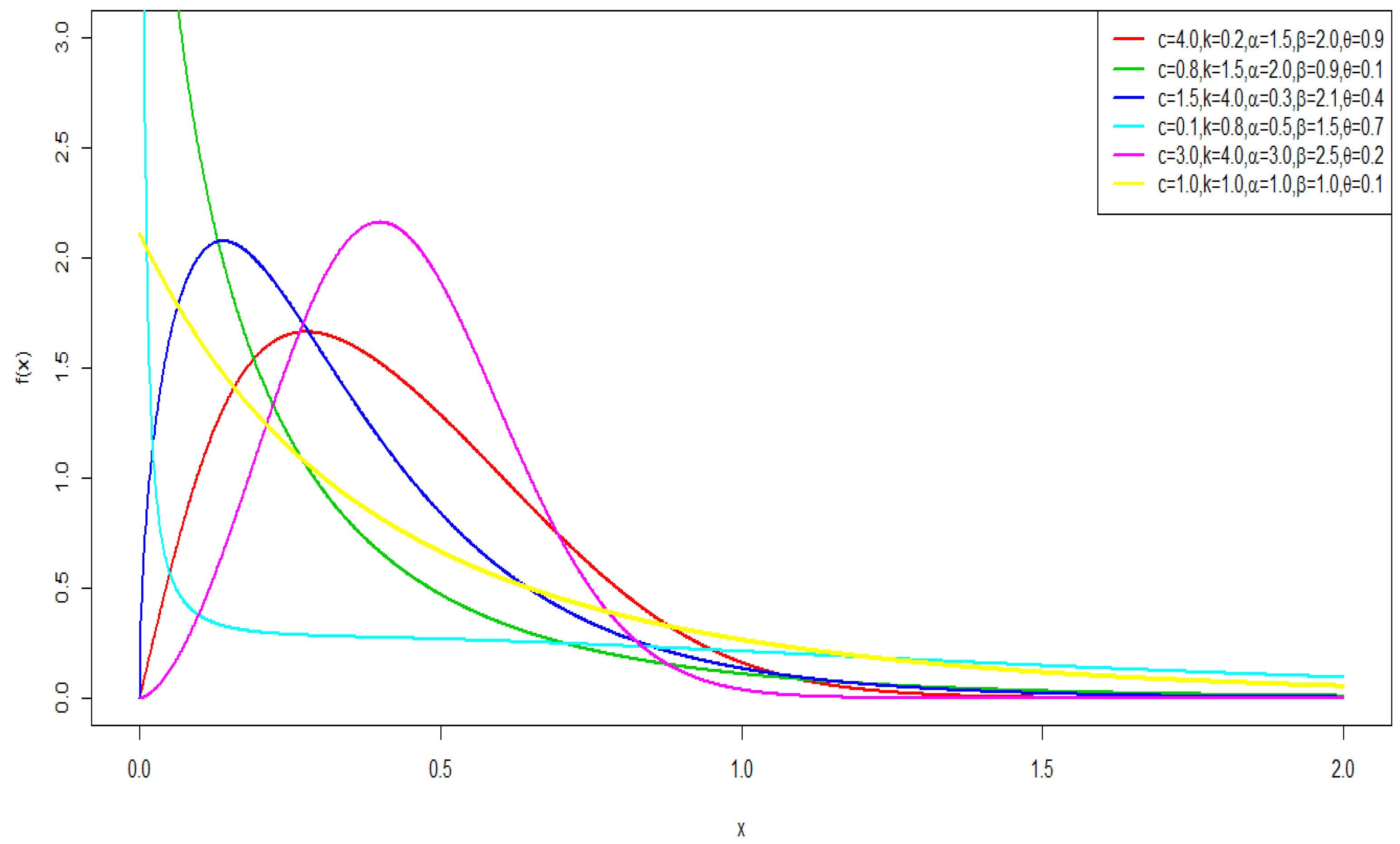
2. Burr XII-Weibull-Logarithmic Distribution
Quantile Function
3. Moments, Conditional Moments and Mean Deviations
3.1. Moments
3.2. Conditional Moments
4. Maximum Likelihood Estimation
Asymptotic Confidence Intervals
5. Simulation Study
- (a)
- Average bias of the MLE of the parameter
- (b)
- Root mean squared error (RMSE) of the MLE of the parameter
- (c)
- Coverage probability (CP) of 95% confidence intervals of the parameter , i.e., the percentage of intervals that contain the true value of parameter .
- (d)
- Average width (AW) of 95% confidence intervals of the parameter .
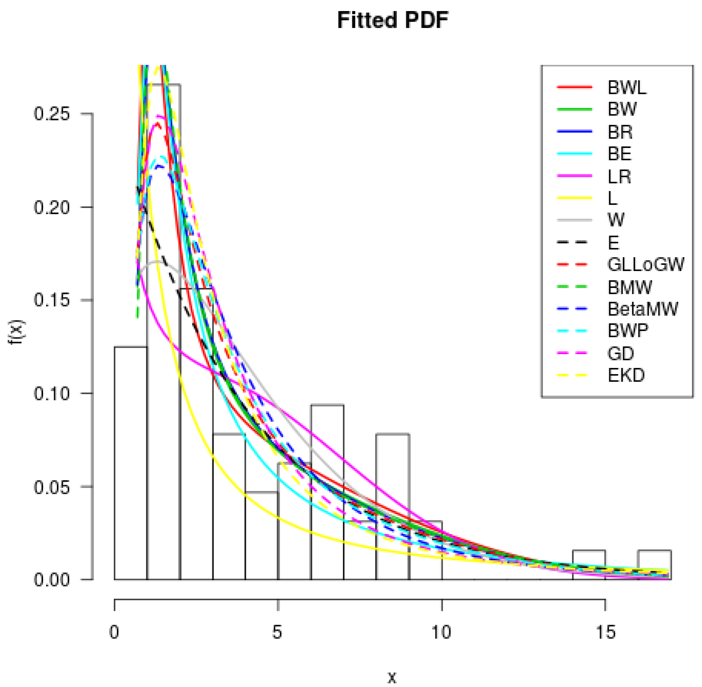
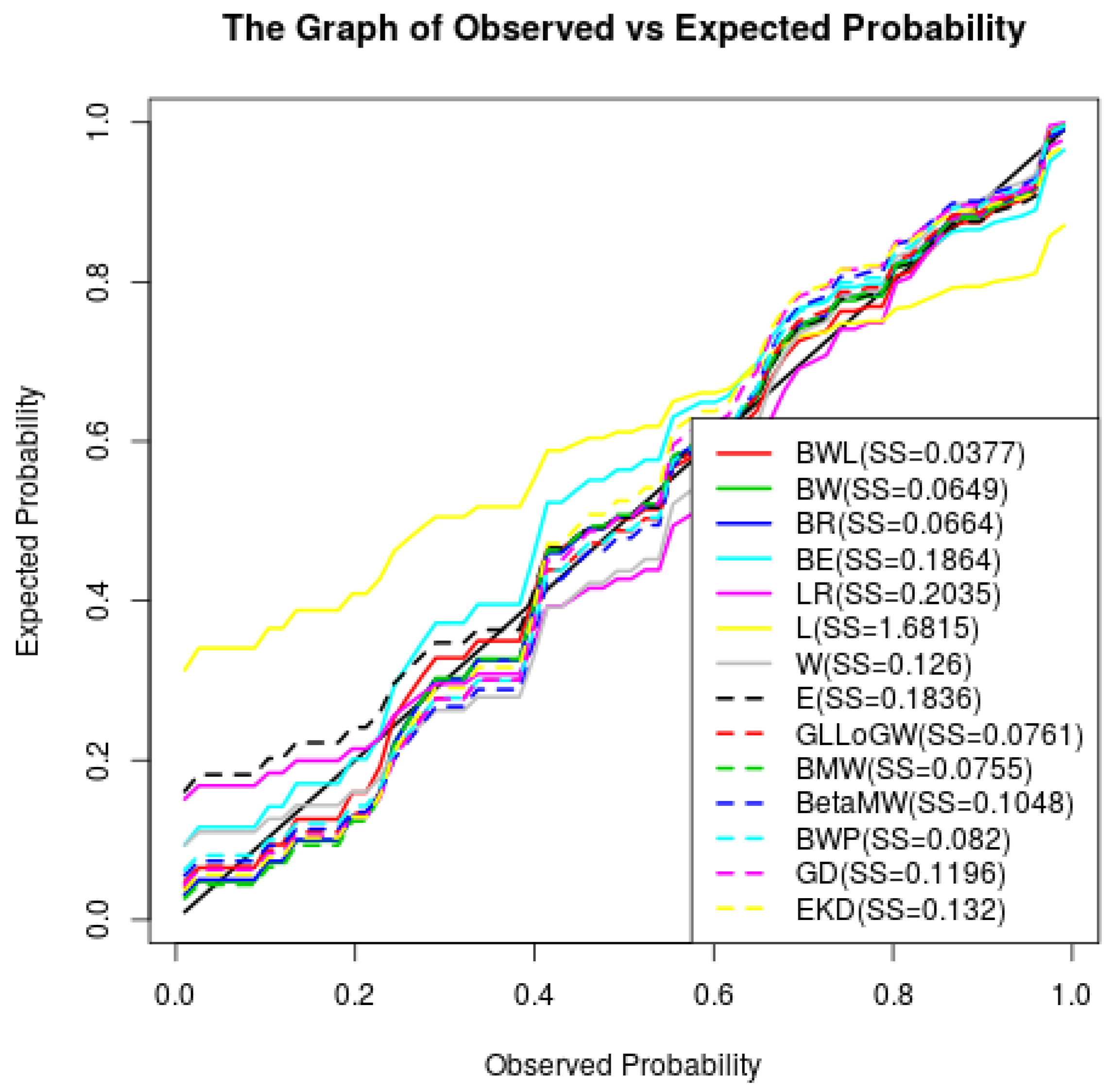
6. Applications
6.1. Waiting Time between Eruptions (Seconds)
6.2. Time to Failure of Kevlar 49/Epoxy Strands Tested at Various Stress Levels
7. Conclusions
Author Contributions
Acknowledgments
Conflicts of Interest
References
- Makubate, B.; Oluyede, B.O.; Motobetso, G.; Huang, S.; Fagbamigbe, A.F. The Beta Weibull-G Family of Distributions: Model, Properties and Application. Int. J. Stat. Probab. 2018, 7, 12–32. [Google Scholar] [CrossRef]
- Oluyede, B.O.; Huang, S.; Mashabe, B.; Fagbamigbe, A.F. A New Class of Distributions for Survival and Lifetime Data Analysis: Theory and Applications. J. Prob. Stat. Soc. 2017, 15, 153. [Google Scholar]
- Morais, A.L.; Barreto-Souza, W. A Compound Class of Weibull and Power Series Distributions. Comput. Stat. Data Anal. 2011, 55, 1410–1425. [Google Scholar] [CrossRef]
- Silva, R.B.; Bourguignon, M.; Dais, C.R.B.; Cordeiro, G.M. The Compound Family of Extended Weibull Power Series Distributions. Comput. Stat. Data Anal. 2013, 58, 352–367. [Google Scholar] [CrossRef]
- Silva, R.B.; Cordeiro, G.M. The Burr XII Power Series Distributions: A New Compounding Family. Braz. J. Probab. Stat. 2013, 29, 565–589. [Google Scholar] [CrossRef]
- Oluyede, B.O.; Warahena-Liyanage, G.; Pararai, M. A New Compound Class of Log-logistic Weibull-Poisson Distribution: Model, Properties and Applications. J. Stat. Comput. Simul. 2015, 86, 1363–1391. [Google Scholar] [CrossRef]
- Tahir, M.H.; Zubair, M.; Mansoor, M.; Cordeiro, G.M.; Alizadeh, M. A new Weibull-G family of distributions. Hacet. J. Math. Stat. 2016, 45, 29–47. [Google Scholar] [CrossRef]
- Oluyede, B.O.; Makubate, B.; Warahena-Liyanage, G.; Ayoku, S. A New Model for Lifetime Data: The Burr XII-Weibull Distribution: Properties and Applications. Unpublished Manuscript. 2018. [Google Scholar]
- Nadarajah, S.; Cordeiro, G.M.; Ortega, E.M.M. General Results for the Beta-Modified Weibull Distribution. J. Stat. Comput. Simul. 2011, 81, 1211–1232. [Google Scholar] [CrossRef]
- Huang, S.; Oluyede, B.O. Exponentiated Kumaraswamy-Dagum Distribution with Applications to Income and Lifetime Data. J. Stat. Distrib. Appl. 2014, 1, 8. [Google Scholar] [CrossRef]
- Percontini, A.; Blas, B.; Cordeiro, G.M. The beta Weibull Poisson distribution. Chil. J. Stat. 2013, 4, 3–26. [Google Scholar]
- Oluyede, B.O.; Huang, S.; Pararai, M. A New Class of Generalized Dagum Distribution with Applications to Income and Lifetime Data. J. Stat. Econ. Methods 2014, 3, 125–151. [Google Scholar]
- Foya, S.; Oluyede, B.O.; Fagbamigbe, A.F.; Makubate, B. The Gamma Log-logistic Distribution: Model, Properties and Application. Electron. J. Appl. Stat. Anal. 2017, 10, 206–241. [Google Scholar]
- R Development Core Team. A Language and Environment for Statistical Computing; R Foundation for Statistical Computing: Vienna, Austria, 2011. [Google Scholar]
- Seregin, A. Uniqueness of the Maximum Likelihood Estimator for k-Monotone Densities. Proc. Am. Math. Soc. 2010, 138, 4511–4515. [Google Scholar] [CrossRef]
- Santos, S.J.M.C.; Tenreyro, S. On the Existence of Maximum Likelihood Estimates in Poisson Regression. Econ. Lett. 2010, 107, 310–312. [Google Scholar] [CrossRef]
- Zhou, C. Existence and Consistency of the Maximum Likelihood Estimator for the Extreme Index. J. Multivar. Anal. 2009, 100, 794–815. [Google Scholar] [CrossRef]
- Xia, J.; Mi, J.; Zhou, Y.Y. On the Existence and Uniqueness of the Maximum Likelihood Estimators of Normal and Log-Normal Population Parameters with Grouped Data. J. Probab. Stat. 2009, 2009. [Google Scholar] [CrossRef]
- Chen, G.; Balakrishnan, N. A General Purpose Approximate Goodness-of-fit Test. J. Qual. Technol. 1995, 27, 154–161. [Google Scholar] [CrossRef]
- Irish, J. Kiama Blowhole Eruptions. Accessed Jan 4, 2008. Available online: http://www.statsci.org/data/oz/kiama.html (accessed on 6 June 2018).
- Cooray, K.; Ananda, M.M.A. A Generalization of the Half-Normal Distribution with Applications to Lifetime Data. Commun. Stat. Theory Method. 2008, 37, 1323–1337. [Google Scholar] [CrossRef]
- Andrews, D.F.; Herzberg, A.M. Data: A Collection of Problems from Many Fields for the Student and Research Worker; Springer Series in Statistics; Springer: New York, NY, USA, 1985. [Google Scholar]
- Barlow, R.E.; Toland, R.H.; Freeman, T. A Bayesian Analysis of Stress-Rupture Life of Kevlar 49/epoxy Spherical Pressure Vessels. In Proceedings of the 5th Canadian Conference in Applied Statistics; Marcel Dekker: New York, NY, USA, 1984. [Google Scholar]


| Parameter | n | I | II | ||||||
|---|---|---|---|---|---|---|---|---|---|
| Average Bias | RMSE | CP | AW | Average Bias | RMSE | CP | AW | ||
| c | 25 | 2.675779 | 8.851342 | 0.994000 | 23.936930 | 1.84205 | 5.301441 | 0.976000 | 18.566570 |
| 50 | 1.101271 | 4.041046 | 0.991000 | 12.25807 | 0.677570 | 2.166961 | 0.991000 | 12.468810 | |
| 75 | 0.776600 | 2.437517 | 0.994000 | 9.070155 | 0.498752 | 1.758328 | 0.989000 | 10.092830 | |
| 100 | 0.535438 | 1.634913 | 0.998000 | 7.341681 | 0.396074 | 1.469932 | 0.996000 | 8.697054 | |
| 200 | 0.263376 | 1.061385 | 0.995000 | 4.845233 | 0.173937 | 1.009647 | 0.991000 | 6.011405 | |
| 400 | 0.156439 | 0.680718 | 0.994000 | 3.304505 | 0.084850 | 0.718829 | 0.995000 | 4.211869 | |
| 800 | 0.061912 | 0.4918901 | 0.986000 | 2.285547 | 0.095066 | 0.570643 | 0.992000 | 2.976686 | |
| 1000 | 0.081336 | 0.452049 | 0.980000 | 2.044596 | 0.095846 | 0.550242 | 0.984000 | 2.659770 | |
| k | 25 | 0.0237202 | 0.494053 | 0.936000 | 3.481823 | 1.369074 | 9.144814 | 0.990000 | 11.460170 |
| 50 | 0.001349 | 0.342498 | 0.951000 | 2.405994 | 0.270353 | 0.915826 | 0.997000 | 5.205493 | |
| 75 | 0.269091 | 0.966000 | 1.904094 | 0.179129 | 0.643348 | 0.995000 | 4.283715 | ||
| 100 | 0.226214 | 0.974000 | 1.652106 | 0.098394 | 0.508880 | 0.995000 | 3.661433 | ||
| 200 | 0.174008 | 0.981000 | 1.149372 | 0.049542 | 0.364229 | 0.995000 | 2.564741 | ||
| 400 | 0.127224 | 0.989000 | 0.804003 | 0.021869 | 0.270349 | 0.997000 | 1.810466 | ||
| 800 | 0.103233 | 0.99000 | 0.566534 | 0.009208 | 0.220733 | 0.994000 | 1.276235 | ||
| 1000 | 0.093743 | 0.989000 | 0.506535 | 0.006077 | 0.204273 | 0.992000 | 1.137812 | ||
| 25 | 0.069957 | 0.310585 | 0.992000 | 4.833469 | 0.121678 | 0.301760 | 0.980000 | 4.541517 | |
| 50 | 0.0430549 | 0.242650 | 0.986000 | 3.694583 | 0.058815 | 0.218128 | 0.982000 | 3.630756 | |
| 75 | 0.031248 | 0.202928 | 0.987000 | 3.015649 | 0.049777 | 0.185170 | 0.978000 | 3.089071 | |
| 100 | 0.016989 | 0.189611 | 0.984000 | 2.599544 | 0.027009 | 0.175936 | 0.975000 | 2.633679 | |
| 200 | 0.008977 | 0.162091 | 0.986000 | 1.862088 | 0.025182 | 0.160722 | 0.981000 | 1.907583 | |
| 400 | 0.010789 | 0.148684 | 0.990000 | 1.307337 | 0.015547 | 0.147112 | 0.987000 | 1.342973 | |
| 800 | 0.006690 | 0.139677 | 0.989000 | 0.919219 | 0.010717 | 0.138944 | 0.993000 | 0.947612 | |
| 1000 | 0.006347 | 0.133964 | 0.992000 | 0.826020 | 0.004011 | 0.129613 | 0.993000 | 0.836210 | |
| 25 | 0.033337 | 0.219043 | 0.973000 | 1.311640 | 0.033815 | 0.166012 | 0.981000 | 0.841818 | |
| 50 | 0.022060 | 0.141783 | 0.991000 | 0.905219 | 0.018499 | 0.085023 | 0.994000 | 0.622538 | |
| 75 | 0.022018 | 0.116760 | 0.983000 | 0.7267897 | 0.009590 | 0.066644 | 0.994000 | 0.503165 | |
| 100 | 0.013218 | 0.100725 | 0.994000 | 0.619022 | 0.011386 | 0.060717 | 0.996000 | 0.439842 | |
| 200 | 0.008977 | 0.073217 | 0.993000 | 0.429614 | 0.007230 | 0.043097 | 0.989000 | 0.309474 | |
| 400 | 0.006178 | 0.052166 | 0.991000 | 0.299177 | 0.003806 | 0.033442 | 0.996000 | 0.216698 | |
| 800 | 0.004166 | 0.041231 | 0.993000 | 0.210559 | 0.003685 | 0.027366 | 0.993000 | 0.153173 | |
| 1000 | 0.005101 | 0.037446 | 0.991000 | 0.188943 | 0.004511 | 0.025963 | 0.996000 | 0.137367 | |
| 25 | 0.339392 | 0.912000 | 8.252486 | 0.379665 | 0.858000 | 7.477688 | |||
| 50 | 0.304801 | 0.939000 | 6.317330 | 0.302833 | 0.936000 | 6.194896 | |||
| 75 | 0.274624 | 0.964000 | 5.125504 | 0.293129 | 0.950000 | 5.591709 | |||
| 100 | 0.266921 | 0.970000 | 4.408751 | 0.271070 | 0.967000 | 4.649491 | |||
| 200 | 0.253383 | 0.983000 | 3.211048 | 0.270891 | 0.978000 | 3.467229 | |||
| 400 | 0.244138 | 0.991000 | 2.269061 | 0.250295 | 0.987000 | 2.412363 | |||
| 800 | 0.234049 | 0.963000 | 1.559317 | 0.245471 | 0.981000 | 1.698596 | |||
| 1000 | 0.227437 | 0.957000 | 1.392764 | 0.228074 | 0.958000 | 1.451740 | |||
| Model | Estimates | Statistics | |||||||||||||
|---|---|---|---|---|---|---|---|---|---|---|---|---|---|---|---|
| c | k | p-Value | |||||||||||||
| BWL | 4.4524 | 0.0451 | 0.0057 | 2.3625 | 0.9051 | 285.78 | 295.78 | 296.82 | 296.82 | 306.58 | 0.0407 | 0.3964 | 0.0614 | 0.9694 | 0.0377 |
| (1.7573) | (0.1032) | (0.0114) | (0.7633) | (0.3623) | |||||||||||
| BW | 4.3730 | 0.1392 | 0.0078 | 2.2103 | 0 | 286.81 | 294.81 | 295.85 | 295.49 | 303.45 | 0.0572 | 0.4874 | 0.0898 | 0.6806 | 0.0649 |
| (1.2190) | (0.0479) | (0.0121) | (0.5851) | - | |||||||||||
| BR | 4.3420 | 0.1332 | 0.0135 | 2 | 0 | 286.98 | 292.98 | 294.01 | 293.38 | 299.45 | 0.0583 | 0.4915 | 0.0890 | 0.6916 | 0.0664 |
| (1.2542) | (0.0453) | (0.0043) | - | - | |||||||||||
| BE | 4.8239 | 0.1011 | 0.1171 | 1 | 0 | 299.21 | 305.21 | 306.25 | 305.61 | 311.69 | 0.1114 | 0.8304 | 0.1171 | 0.3440 | 0.1864 |
| (1.7590) | (0.0589) | (0.0578) | - | - | |||||||||||
| LR | 1 | 0.2893 | 0.0219 | 2 | 0 | 310.00 | 314.00 | 315.04 | 314.20 | 318.32 | 0.2418 | 1.5705 | 0.1525 | 0.1020 | 0.2035 |
| - | (0.0866) | (0.0049) | - | - | |||||||||||
| L | 1 | 0.7085 | 0 | 0.1000 | 0 | 352.77 | 356.77 | 357.80 | 356.96 | 361.08 | 0.1234 | 0.9002 | 0.3250 | 0.0000 | 1.6815 |
| - | (0.0886) | - | (7.266566E–17) | - | |||||||||||
| W | 0.1000 | 0 | 0.1549 | 1.2744 | 0 | 299.07 | 305.07 | 306.10 | 305.47 | 311.55 | 0.1471 | 1.0080 | 0.1113 | 0.4061 | 0.1260 |
| (2.255944E–12) | - | (0.0392) | (0.1203) | - | |||||||||||
| E | 0.1000 | 0 | 0.2511 | 1 | 0 | 304.89 | 308.89 | 309.93 | 309.09 | 313.21 | 0.1317 | 0.9179 | 0.1664 | 0.0579 | 0.1836 |
| (5.176341E–18) | - | (0.0314) | - | - | |||||||||||
| c | |||||||||||||||
| GLLoGW | 1.4725 | 0.0042 | 2.4336 | 0.7650 | 0.3841 | 289.79 | 299.79 | 300.82 | 300.82 | 310.58 | 0.0694 | 0.5695 | 0.0901 | 0.6759 | 0.0761 |
| (1.1419) | (0.0316) | (2.0826) | (1.3339) | (0.4998) | |||||||||||
| c | k | ||||||||||||||
| BMW | 4.8935 | 0.1186 | 0.0155 | 1.8669 | 0.0150 | 287.33 | 297.33 | 298.36 | 298.36 | 308.12 | 0.0640 | 0.5233 | 0.0952 | 0.6080 | 0.0755 |
| (1.5277) | (0.0482) | (0.0229) | (0.9151) | (0.1010) | |||||||||||
| a | b | ||||||||||||||
| BetaMW | 479.79 | 81.242 | 1.8115 | 0.0569 | 0.0017 | 292.56 | 302.56 | 303.59 | 303.59 | 313.35 | 0.1007 | 0.7420 | 0.1018 | 0.5207 | 0.1048 |
| (0.0000) | (0.0002) | (0.0161) | (0.0100) | (0.0023) | |||||||||||
| a | b | ||||||||||||||
| BWP | 0.9655 | 1.7087 | 0.0023 | 2.4690 | 6.8923 | 292.75 | 302.75 | 303.79 | 303.79 | 313.55 | 0.0881 | 0.6810 | 0.0905 | 0.6706 | 0.0820 |
| (0.4813) | (1.0119) | (0.0085) | (1.3350) | (5.0272) | |||||||||||
| GD | 0.4870 | 3.9072 | 0.4828 | 5.0474 | 0.0950 | 293.40 | 303.40 | 304.44 | 304.44 | 314.20 | 0.1148 | 0.8419 | 0.0942 | 0.6212 | 0.1196 |
| (0.7748) | (5.9018) | (0.4452) | (7.6696) | (0.1790) | |||||||||||
| EKD | 16.331 | 0.1746 | 0.1739 | 31.136 | 22.357 | 293.87 | 303.87 | 304.90 | 304.90 | 314.66 | 0.1295 | 0.9353 | 0.0980 | 0.5699 | 0.1320 |
| (11.382) | (0.1352) | (0.0173) | (1.1928) | (0.7287) | |||||||||||
| Model | Estimates | Statistics | |||||||||||||
|---|---|---|---|---|---|---|---|---|---|---|---|---|---|---|---|
| BWL | 5.8331 | 0.2335 | 0.4260 | 0.7695 | 0.7290 | 196.12 | 206.12 | 206.75 | 206.75 | 219.19 | 0.0429 | 0.3107 | 0.0516 | 0.9505 | 0.0419 |
| (2.0868) | (0.1268) | (0.3959) | (0.1738) | (0.5967) | |||||||||||
| LEL | 1 | 1.5648 | 4.522787E–05 | 4.3566 | 0.0971 | 220.28 | 228.28 | 228.91 | 228.69 | 238.74 | 0.4746 | 2.5587 | 0.1572 | 0.0136 | 0.5814 |
| - | (0.2561) | (0.0001) | (0.0330) | (0.4110) | |||||||||||
| EL | 0.1000 | 0 | 0.9255 | 1 | 0.1900 | 206.88 | 212.88 | 213.52 | 213.13 | 220.73 | 0.1952 | 1.0971 | 0.0834 | 0.4838 | 0.1770 |
| (2.011761E–15) | - | (0.2034) | - | (0.6219) | |||||||||||
| BW | 0.7099 | 0.4274 | 0.6842 | 1.1195 | 0 | 205.72 | 213.72 | 214.35 | 214.13 | 224.18 | 0.1541 | 0.9121 | 0.0815 | 0.5141 | 0.1526 |
| (0.2174) | (0.6220) | (0.4694) | (0.3497) | - | |||||||||||
| BR | 1.0054 | 1.3175 | 0.0907 | 2 | 0 | 210.98 | 216.98 | 217.61 | 217.22 | 224.82 | 0.2492 | 1.3902 | 0.1020 | 0.2442 | 0.2396 |
| (0.1247) | (0.2130) | (0.0471) | - | - | |||||||||||
| BE | 0.6774 | 0.2007 | 0.8595 | 1 | 0 | 205.82 | 211.82 | 212.45 | 212.07 | 219.66 | 0.1779 | 1.0171 | 0.0875 | 0.4222 | 0.1773 |
| (0.2778) | (0.2342) | (0.1596) | - | - | |||||||||||
| LR | 1 | 1.3136 | 0.0919 | 2 | 0 | 210.98 | 214.98 | 215.61 | 215.10 | 220.21 | 0.2471 | 1.3808 | 0.1020 | 0.2445 | 0.2385 |
| - | (0.1928) | (0.0383) | - | - | |||||||||||
| L | 1 | 1.6638 | 0 | 0.1000 | 0 | 220.56 | 224.56 | 225.20 | 224.69 | 229.79 | 0.4702 | 2.5406 | 0.1663 | 0.0075 | 0.6549 |
| - | (0.1656) | - | (1.223928E–16) | - | |||||||||||
| W | 0.1000 | 0 | 1.0094 | 0.9259 | 0 | 205.95 | 211.95 | 212.59 | 212.20 | 219.80 | 0.1987 | 1.1111 | 0.0906 | 0.3778 | 0.1954 |
| (1.523294E–16) | - | (0.1053) | (0.0726) | - | |||||||||||
| R | 0.1000 | 0 | 0.4365 | 2 | 0 | 360.46 | 364.46 | 365.09 | 364.58 | 369.69 | 0.1206 | 0.9184 | 0.2711 | 0.0000 | 3.5326 |
| (3.377936E–16) | - | (0.0434) | - | - | |||||||||||
| c | |||||||||||||||
| GLLoGW | 0.2365 | 0.2591 | 0.9648 | 4.3962 | 0.1396 | 204.01 | 214.01 | 214.64 | 214.64 | 227.08 | 0.1322 | 0.7996 | 0.0752 | 0.6173 | 0.1289 |
| (0.2965) | (0.3727) | (0.3741) | (10.719) | (0.3332) | |||||||||||
| a | b | ||||||||||||||
| BetaMW | 108.86 | 25.631 | 1.6632 | 0.0534 | 0.0343 | 207.31 | 217.31 | 217.94 | 217.94 | 230.38 | 0.1955 | 1.1190 | 0.0932 | 0.3437 | 0.1916 |
| (0.0002) | (0.0009) | (0.0279) | (0.0075) | (0.0089) | |||||||||||
| a | b | ||||||||||||||
| BWP | 0.0745 | 8.3950 | 0.8247 | 1.0698 | 374.51 | 202.04 | 212.04 | 212.67 | 212.67 | 225.12 | 0.1141 | 0.7016 | 0.0706 | 0.6961 | 0.1093 |
| (0.0177) | (0.3903) | (0.2761) | (0.2005) | (0.0015) | |||||||||||
| GD | 49.090 | 0.3216 | 9.9094 | 0.2055 | 6.8443 | 196.58 | 206.58 | 207.21 | 207.21 | 219.66 | 0.0367 | 0.2895 | 0.0586 | 0.8788 | 0.0352 |
| (111.98) | (0.2286) | (5.0965) | (0.1636) | (6.1399) | |||||||||||
| EKD | 0.0179 | 6.7074 | 3.7473 | 0.8577 | 8.4926 | 199.84 | 209.84 | 210.48 | 210.48 | 222.92 | 0.0553 | 0.4193 | 0.0640 | 0.8024 | 0.0581 |
| (0.0279) | (6.5531) | (0.9489) | (0.2534) | (13.328) | |||||||||||
© 2018 by the authors. Licensee MDPI, Basel, Switzerland. This article is an open access article distributed under the terms and conditions of the Creative Commons Attribution (CC BY) license (http://creativecommons.org/licenses/by/4.0/).
Share and Cite
Oluyede, B.O.; Makubate, B.; Fagbamigbe, A.F.; Mdlongwa, P. A New Burr XII-Weibull-Logarithmic Distribution for Survival and Lifetime Data Analysis: Model, Theory and Applications. Stats 2018, 1, 77-91. https://doi.org/10.3390/stats1010006
Oluyede BO, Makubate B, Fagbamigbe AF, Mdlongwa P. A New Burr XII-Weibull-Logarithmic Distribution for Survival and Lifetime Data Analysis: Model, Theory and Applications. Stats. 2018; 1(1):77-91. https://doi.org/10.3390/stats1010006
Chicago/Turabian StyleOluyede, Broderick O., Boikanyo Makubate, Adeniyi F. Fagbamigbe, and Precious Mdlongwa. 2018. "A New Burr XII-Weibull-Logarithmic Distribution for Survival and Lifetime Data Analysis: Model, Theory and Applications" Stats 1, no. 1: 77-91. https://doi.org/10.3390/stats1010006
APA StyleOluyede, B. O., Makubate, B., Fagbamigbe, A. F., & Mdlongwa, P. (2018). A New Burr XII-Weibull-Logarithmic Distribution for Survival and Lifetime Data Analysis: Model, Theory and Applications. Stats, 1(1), 77-91. https://doi.org/10.3390/stats1010006