Article

Causality between Oil Prices and Tourist Arrivals

1
Faculty of Business and Law, De Montfort University, Leicester LE1 9BH, UK
2
Fashion Business School, London College of Fashion, University of the Arts London, London WC1V 7EY, UK
3
Research Institute of Energy Management and Planning, University of Tehran, Tehran 1417466191, Iran
*
Author to whom correspondence should be addressed.
Stats 2018, 1(1), 134-154; https://doi.org/10.3390/stats1010010
Submission received: 19 September 2018 / Revised: 16 October 2018 / Accepted: 16 October 2018 / Published: 20 October 2018

Abstract

:
This paper investigates the causal relationship between oil price and tourist arrivals to further explain the impact of oil price volatility on tourism-related economic activities. The analysis itself considers the time domain, frequency domain, and information theory domain perspectives. Data relating to the US and nine European countries are exploited in this paper with causality tests which include the time domain, frequency domain, and Convergent Cross Mapping (CCM). The CCM approach is nonparametric and therefore not restricted by assumptions. We contribute to existing research through the successful and introductory application of an advanced method and via the uncovering of significant causal links from oil prices to tourist arrivals.

1. Introduction

Oil price movements can significantly affect countries that are heavily reliant on the tourism industry, and research indicates that such countries are unevenly exposed to sudden fluctuations in oil prices [1]. The harmful effects of oil price fluctuations on transportation, production costs, economic uncertainty, and disposable income [2] have long been discussed. In the recent past it was oil prices hikes that influenced investigations into the relationship between tourism and oil price fluctuations [3]. However, today, it is falling oil prices that continue to necessitate further investigations, and given the tourism industry’s energy-intensive nature [2,3], it is not surprising that the relationship between oil prices and tourist arrivals remains a crucial research topic. The emerging concerns relating to oil prices and its impact on diverse aspects of industrial economies have been studied by numerous researchers [4,5,6,7,8,9,10,11,12,13,14,15]. Among this research, the relationship between oil price and tourism has drawn significant attention [1,2,16,17], and this is understandable as tourism is recognized as the third largest industry in the world after oil and automobiles [18].
The accurate detection of causality between oil prices and tourist arrivals can help the tourism planning process and aid in improving the quality of tourist arrival forecasts and related managerial decisions [19]. Whilst econometric tourism models are acknowledged for having a lower empirical cost, there is strong evidence which portrays the importance of quantitative causal econometric models in enabling a better understanding of the factors affecting tourism demand [20,21]. Moreover, past literature indicates a negative association between oil price and tourism [1,16], which is supported by overwhelming evidence from factors like inflation, Consumer Price Index (CPI), oil production, tourism income, and industrial production indices.
The aim of this paper is to further evaluate this oil-tourism relationship and efficiently investigate the existence of causal links by conducting data-driven research with an advanced nonparametric method known as Convergent Cross Mapping (CCM) [22]. Instead of building a complex model by incorporating many possible influential variables based on regression modelling, which is restricted by the number of assumptions, this paper adopts CCM which is popular due to its significant sensitivity in detecting causal links within complex systems whilst not being restricted by assumptions pertaining to linearity or nonlinearity. Moreover, we intend to use this research to reflect the inherent efficiency and power of CCM in relation to empirical tests to further promote its use in the future. Accordingly, we seek to find significant evidence of oil–tourism causal relationships on a global scale by involving only the two key variables —oil price and tourist arrivals alone. A better understanding of this relationship with a more efficient and complex dynamic applicable approach will help to identify, compare and monitor the level of dependence so to assist in policy making and adjustments in tourism economics.
The results from CCM are compared with two empirical causality methods which fall under the time domain and frequency domain criteria. To the best of our knowledge, this paper marks the introduction and successful adoption of CCM for identifying causality between the oil price and tourist arrivals. Accordingly this research presents three contributions to scientific literature on the relationship between oil and tourism. Firstly, our research focuses on a data-driven investigation of causal effects across both US and nine European countries via the introductory application of CCM. Secondly, we consider monthly data in our analysis, and this is important as such data is seldom used in the analysis of causal relationships between tourism demand and its influencing factors [23,24]. Thirdly, our findings enable us to prove that this advanced and assumption free CCM causality test is a robust, solid, and efficient method that can produce reliable evidence by using only two key variables. As such, it is possible to introduce CCM as a method with great potential for other causal analyses in tourism studies and more importantly in a broader range of subjects.
The remainder of this paper is organized as follows. Section 2 presents a literature review which is followed by Section 3 where we briefly introduce both the empirical and advanced causality detection techniques. Section 4 provides the descriptive analyses of oil price and tourist arrival data across the US and nine European countries, along with the unit root test results. The causality test results are summarized in Section 5, and the paper concludes in Section 6.

2. Literature Review

A critical review of the studies on tourism and oil can be found in [25], and therefore, these are not reproduced here. Instead, we focus mainly on the more recent causality testing applications related to tourist arrivals from 2012 onwards, and these are reviewed in chronological order, capturing the different techniques that have been developed and exploited in the recent past.
Causality between foreign direct investment (FDI) and tourist arrivals in India was evaluated with the aid of a Granger causality test under a Vector Autoregression (VAR) framework in [26] where the authors found a two-way causality link between FDI and tourist arrivals in India. A Granger causality test with an Error Correction Model (ECM) was used in [27] to find causal relationships between international tourist arrivals, GDP, and trade in Italy, whilst a recursive Granger causality test with an ECM was used in [28] to verify the tourism-led growth hypothesis in Malaysia with respect to different tourism markets. They found that the tourism-led growth hypothesis in Malaysia is valid and stable with respect to tourist arrivals from only eight out of the 12 tourism markets [28]. In the case of Jamaica, stepwise Granger causality tests for short run causality and Granger causality within the Vector Error Correction Modelling (VECM) framework for long-run causality were exploited in [29] as the authors endeavoured to find causal relationships between tourism, growth, real exchange rates, structural changes, and hurricanes. In [30], the authors exploited a Granger causality test on Italian data which showed that bi-directional causality exists in the long-run dynamics of visits to museums and monuments that mainly adjust to tourism variables (arrivals, overnights, average stays), whilst in the short run, there are some causal effects going from cultural site attendance to tourism dynamics.
A multivariate Granger causality test based on an ECM was adopted in [31] where the authors found a a two-way causal relationship between real GDP growth and tourism growth in Spain with Granger causality running from Spanish real GDP to tourist arrivals, and Granger causality running from foreign real GDP to Spanish real GDP, tourist arrivals, and the ratio of luxury hotels to the total number of hotels in Spain. In [32], a Granger causality test through block exogeneity wald tests under the ECM mechanism was used to show the existence of unidirectional causality that runs from tourism development to carbon emission growth in the long-term of the economy of Singapore. Conditional Granger causality tests under the ECM and Autoregressive Distributed Lag (ARDL) models were used in [33] to show that international tourism is a catalyst for energy consumption and for an increase in the level of carbon dioxide emissions in Cyprus. The existence of a causal link between tourism and economic growth in Lebanon was investigated via a bounds testing approach to cointegration and Granger causality tests in [34], and the authors uncovered that the tourism-led growth hypothesis is valid for Lebanon. Panel Granger causality tests were used in [35] to show the existence of a bi-directional causal relationship between foreign direct investment in real estate and international tourism in Organization for Economic Co-operation and Development (OECD) countries. A VECM Granger causality test was used in [36] to uncover unidirectional long-run causality running from tourist arrivals to pollution in Malaysia, but the authors failed to establish any causal relationship between tourism and economic growth in the long-run.
A Vector Autoregression-based spillover index approach was used in [37] to examine the time-varying spillover effects between tourism and economic growth in Europe. The authors found that the tourism-economic growth relationship is very responsive to major economic events and as such, varies over time in terms of both magnitude and direction. A standard Granger causality test was adopted in [38] to determine the drivers of Taiwan’s tourism market cycle, whilst a block Granger causality test was adopted in [24] along with an unconstrained VAR to identify the causal relationships underlying tourism demand for the city of Paris originating from its five major source markets (Germany, Italy, Japan, United Kingdom, and United States). A Granger causality test with VECM was exploited in [39] to determine the causal relationship between tourist arrivals and economic growth in Malaysia. They found that in the short run, tourism and economic growth Granger cause each other in Malaysia with a uni-directional causality running from tourism to economic growth in the long run. In [40], the authors used tourism receipts as a proxy for tourist arrivals and searched for causal relationships between tourism receipts and GDP in Spain and the UK using a copula-based Generalized Autoregressive Conditional Heteroskedasticity (GARCH) model. They found a positive relationship between tourism receipts and the GDP level and concluded that stimulating the tourism sector can lead to economic growth. Using monthly data for international tourist arrivals in 10 European countries as a proxy for tourism performance, the authors of [41] carried out Granger causality tests and found that the tourism led economic growth hypothesis is evident only for Italy and the Netherlands, while economic-driven tourism growth is observed in Cyprus, Germany, and Greece, in addition to evidence of bidirectional causality in the cases of Austria, Portugal, and Spain, while no causality was identified for Sweden and the UK.
Dumitrescu–Hurlin causality tests were used in [42] to expose the causal relationships between gas emissions, economic growth, energy consumption, tourist arrivals, and trade in OECD countries. They found evidence of uni-directional causality from tourist arrivals to gas emissions, economic growth, energy consumption, and trade. In [43], the authors found bi-directional causality between tourism and output per capita, financial development and tourism, and trade openness and tourism demand via a Granger causality test with the VECM framework. A panel Granger causality test based on the VECM model was called upon in [44] to find the relationship between tourist arrivals and carbon dioxide emissions in the transportation sectors of a variety of countries. The application of a Granger causality test in [45] indicated a one-way directional causality from tourist arrivals to emissions. In [46], the authors used a Granger causality test within the ECM framework to show long-run unidirectional causality running from tourism to economic growth in Turkey. The application of a rolling Granger causality test confirmed that the tourism led growth hypothesis is valid for Malaysia and that there is evidence of unidirectional causality from tourism to economic growth [47].
An Engle–Granger VAR model was used in [48] where the authors found that business travel Granger-causes trade volumes between Hong Kong and Mainland China, as well as between Hong Kong and Taiwan in addition to the US, illustrating bidirectional causality between business travel and travel volumes for Hong Kong. A Dumitrescu–Hurlin Panel Causality Test was employed in [49] to show the existence of tourism-induced carbon emissions, growth led tourism and health led tourism development in the region, among others by exploiting the cross-sectional panel data of thirty-four countries. A multivariate Granger causality test was used in [50], and they found that Granger causality runs from tourism development and poverty to growth, and from growth and poverty to tourism development, in the case of Madagascar. The causal relationship between tourism and economic growth was evaluated in [51] using a multivariate Granger causality test with the Modified Wald (MWALD) approach [52,53], and they found uni-directional Granger causality running from the real exchange rate to tourism and economic growth in Lebanon. A bivariate Granger causality test was adopted in [54] which showed a significant causation between the composite climate variable index and seasonal variation, a relationship which could be useful for identifying the changes in the fluctuations in tourist arrivals from one season to another. The impact of tourism on economic performance in the UAE was evaluated in [55] via a bootstrapped Granger causality test within the VAR framework, and the authors found evidence for the tourism-led growth hypothesis in the UAE.
Granger causality was used most recently in [56] to find causal relationships between Beijing tourist visitor volumes and a search trend index. Their findings showed that searching for trend data led to the actual Beijing tourist volumes. In [57], an asymmetric Granger causality test based on the VAR system was used to to determine whether Australian inbound and outbound tourism flows across 49 countries are driven by the sign dependent variations in departure series or vice versa. Their findings indicated that changes in departures and arrivals are interrelated for a number of countries.
The literature reviewed here not only shows that CCM is yet to be exploited for the evaluation of causality between tourism and related variables, but also that Granger causality continues to remain a key method for assessing causality between tourist arrivals and influential variables. Whilst it is not the intention of this paper to ridicule any statistical test, we believe it is pertinent to note few drawbacks underlying the Granger causality approach. Firstly, these tests continue to be initially conducted based on a complex model involving many variables, and the principle of the model has not been improved much from simply linear or some assumed specific regressions. Secondly, the conclusion of causality is only obtained by conducting a few tests in a certain order, and these tests are all restricted by various assumptions which can make the process extremely unreliable under real world conditions. On the other hand, CCM, which is proposed in our research, is nonparametric and can find statistically significant evidence for causality by considering only two key variables. Additionally, the calculation itself is efficient and comparatively straight forward with no requirements for involving a variety of influential variables or building a complex model.

3. Methodology of Causality Tests

3.1. Time Domain Granger Causality

The Granger causality test [58] is the most generally accepted and significant method for causality analyses in various disciplines. Ref. [58] focused on the incremental predictability for answering the question of the definition of causality and he proposed a statistical approach, the Granger causality test, which is the most general and significant method for testing the causality relationship between two variables in the linear regression model. Granger suggested that “causality” is testable by simple regression or correlation techniques in two-variable models. Various applications and developments of this technique, including the biomedical area specifically, can be found in [52,59,60,61,62,63,64,65,66].
In addition, a simple Granger causality, the instantaneous Granger causality, and a feedback model are also discussed, where current as well as past values of x are used to predict y t . If y is related to current or lagged x but not future x, then x is exogenous relative to y. The details of Granger’s approach to causality testing are listed as follows; this information primarily follows [58].
Assume there are two stationary stochastic time series X and Y, let I t be the set of all the information in the universe accumulated since time t 1 , so I t Y t denotes all of the information apart from series Y t , and let σ 2 be the corresponding forecast error. X t ¯ represents the set of past values { X t j , j = 1 , 2 , , } , and X t ¯ ¯ represents the set of past and present values { X t j , j = 0 , 1 , 2 , , } . Thus, σ 2 ( X | I t ¯ ) will be the prediction of X using all of the information from the past, and σ 2 ( X | I t Y t ¯ ) will be the prediction of X, using all of the information from the past, apart from series Y.
  • Simple Granger Causality
    If the forecast error of X based on all the information I is smaller than the forecast error of X based on the past information apart from series Y, which is denoted as σ 2 ( X | I t ) < σ 2 ( X | I t Y t ¯ ) , then Y is causing X. Ref. [58] stated, “if we are better able to predict X using all available information than if the information apart from Y had been used, we say that Y is causing X”.
  • Feedback Model
    If the Simple Granger Causality from Y to X is donated as Y X , then the feedback indicates that when X is causing Y and also Y is causing X, which can be represented as X Y , can also be denoted as the following:
    if σ 2 ( X | I ¯ ) = σ 2 ( X | I Y ¯ ) and σ 2 ( Y | I ¯ ) = σ 2 ( Y | I X ¯ ) , then we say X Y .
  • Instantaneous Granger Causality
    Instantaneous causality is indicated if a better forecast of current value of X can be conducted when the present value of Y is also considered, rather than only considering the set of past information. This can be donated as the following: if σ 2 ( X | I ¯ , Y ¯ ¯ ) , the instantaneous causality of Y t X t is occurring.
Another significant definition proposed is the “causality lag” [58]. This states that the lowest value of k such that σ 2 ( X | I Y ( k ) ) < σ 2 ( X | I Y ( k + 1 ) ) is defined as the (integer) causality lag m, which also indicates that the values Y t j , j = 0 , 1 , , m 1 can provide no additional help in improving the forecast of X t .
The regression formulation of Granger causality states that a variable X is the cause of another variable Y if the past values of X are helpful for predicting the future value of Y; two regressions are considered as follows:
Y ( t ) = l = 1 L π l Y ( t l ) + ε 1 , Y ( t ) = l = 1 L π l Y ( t l ) + l = 1 L γ l X ( t l ) + ε 2 ,
where L is the maximal time lag, π and γ are vectors of coefficients, and ε is the prediction error term. If the second is a significantly better model than the first, it can be stated that time series X Granger causes time series Y.

3.2. Frequency Domain Causality

The frequency domain causality test is an extension of the time domain Granger causality (GC) test that identifies the causality between different variables for each frequency. It was firstly proposed by [67], and it permits causality dynamics to be investigated at different frequencies rather than relying on a single statistics as is the case with the conventional time domain analysis [68]. Ref. [69] improved this approach by calculating the GC for each individual frequency component separately instead of computing a single GC measure for the entire relationship, making it possible to determine whether the predictive power is concentrated at the quickly fluctuating components or at the slowly fluctuating components. In order to briefly introduce the testing methodology, we mainly follow [67,68,69].
It is assumed that a two dimensional vector exists containing X i and Y i (where i = 1 , 2 , , N and N is the number of observations) with a finite-order VAR model representative of order p,
Θ ( R ) Y i X i = Θ 11 ( R ) Θ 12 ( R ) Θ 21 ( R ) Θ 22 ( R ) Y i X i + E i ,
where Θ ( R ) = I Θ 1 R Θ p R p is a 2 × 2 lag polynomial, and Θ 1 , , Θ p are 2 × 2 autoregressive parameter matrices with R k X i = X i k and R k Y i = Y i k . The error vector E is white noise with a zero mean, and E ( E i E i ) = Z , where Z is a positive definite matrix. The moving average (MA) representative of the system is
Y i X i = Ψ ( R ) η i = Ψ 11 ( R ) Ψ 12 ( R ) Ψ 21 ( R ) Ψ 22 ( R ) η 1 i η 2 i ,
with Ψ ( R ) = Θ ( R ) 1 G 1 . G is the lower triangular matrix of the Cholesky decomposition G G = Z 1 , such that E ( η t η t ) = I and η i = G E i . The causality test developed in [67] can be written as
C X Y ( γ ) = l o g 1 + | Ψ 12 ( e i γ ) | 2 | Ψ 11 ( e i γ ) | 2 .
However, according to this framework, no Granger causality from X i to Y i at frequency γ corresponds to the condition | Ψ 12 ( e i γ ) | = 0 ; this condition leads to
| Θ 12 ( e i γ ) | = | k = 1 p Θ k , 12 cos ( k γ ) i k = 1 p Θ k , 12 sin ( k γ ) | = 0 ,
where Θ k , 1 , 2 is the ( 1 , 2 ) t h element of Θ k , such that a sufficient set of conditions for no causality is given by [69]
k = 1 p Θ k , 1 , 2 cos ( k γ ) = 0 k = 1 p Θ k , 1 , 2 sin ( k γ ) = 0 .
Hence, the null hypothesis of no Granger causality at frequency γ can be tested with a standard F-test for the linear restrictions (6), which follows a F ( 2 , B 2 p ) distribution, for every γ between 0 and π , with B being the number of observations in the series.

3.3. Convergent Cross Mapping (CCM)

CCM was introduced in [22] with the aim of detecting the causation among time series and providing a better understanding of the dynamical systems that are not covered by other well established methods like Granger causality. CCM has proven to be an advanced, nonparametric technique for distinguishing causation in dynamic systems that contain complex interactions, for example, in biological studies and ecosystems. Those interested in more details are referred to [22,70,71,72]. CCM is briefly introduced below by mainly following [22].
Assume there are two variables X t and Y t , such that X t has a causal effect on Y t , where t = 1 , 2 , , N and N is the total number of observations of the two variables. CCM tests the causality by evaluating whether the historical record of Y t can be used to get reliable reconstructions of X t . Given a library set of n points that are not necessarily equal to the total number of observations N, t = 1 , 2 , , n , the lagged coordinates (lag = τ ) are adopted to generate an E-dimensional embedding state space in which the points are the library vector X t and prediction vector Y t (more details that explicitly discuss the time lags for CCM can be found in [71].)
X t : { x t , x t τ , x t 2 τ , , x t ( E 1 ) τ } ,
Y t : { y t , y t τ , y t 2 τ , , y t ( E 1 ) τ } .
The E + 1 neighbors of Y t from the library set X t are selected, which actually form the smallest simplex that contains Y t as an interior point. Note that the optimal E is evaluated and selected based on the forward performances of these nearby points in an embedding state space. Accordingly, the forecast is then conducted by the nearest-neighbour forecasting algorithm of simplex projection, as listed below in accordance with [73].
Assume an observed time series X t R m + 1 and donate the time series value T p time steps forward as X t + T p ( 1 ) = Y t , so the forecast at T p is
Y ^ t = j = 1 m C t ( j ) X t ( j ) .
The Singular Value Decomposition (SVD) solution for C is obtained using historical points from the fitting set or library set i by B = A C , where
B i = ω ( X i X t ) Y i ,
A i j = ω ( X i X t ) X i ( j ) ,
ω ( d ) = e θ d / d ¯ ,
where θ 0 , d is the distance between the predictee and the neighbour vector, and the scale factor d ¯ is the average distance between neighbours.
Therefore, by adopting the essential concept of empirical dynamic modeling and generalized Taken’s Theorem [74], two manifolds are conducted based on the lagged coordinates of the two variables under evaluation, which are the attractor manifold M Y constructed by Y t and, respectively, the manifold M X by X t . The causation is then identified accordingly if the nearby points on M Y can be employed to reconstruct the observed X t . Note that the correlation coefficient ρ is used for the estimates of the cross map skill due to its wide acceptance and understanding. Additionally, leave-one-out cross-validation is considered a more conservative method and is adopted for all evaluations in CCM.

4. Data

The data used for this paper had a monthly frequency covering the period from January 1996 to December 2015 for both the US and nine European countries, including Austria, Italy, Germany, Greece, Netherland, Portugal, Spain, Sweden, and the UK. In terms of the data, US tourist arrivals were obtained from the US Department of Commerce National Travel & Tourism Office, while data for the European countries were obtained from Eurostat. The data for oil prices included both the West Texas Intermediary Crude Oil Spot Price (WTI) and the Europe Brent Spot Price (BRT) measured in units of dollars per barrel and were obtained via the US Energy Information Administration [75]. Figure 1 shows the time series plots of the monthly oil prices, whilst Figure 2 presents the time series plots of the monthly tourist arrivals by country. It can be observed that the WTI and BRT oil prices were very similar, except for a few months whereby the BRT reported a slightly higher price in relation to the WTI. The impacts of several structural breaks are also visible. In terms of the tourist arrivals data for the ten countries considered (Figure 2), it is evident that these series portray high levels of seasonality and increasing trends over time with some countries showing signs of structural breaks. Figure 1 and Figure 2 further portray the importance of using nonparametric tools in to analyze this data as structural breaks are known for making time series nonstationary [76].

4.1. Descriptive Statistics

The summary of descriptive statistics are listed in Table 1. The data sets include 240 monthly observations for each variable. The descriptive statistics clearly confirm the similarity between the BRT and WTI oil prices. In terms of tourist arrivals, all countries generally showed almost identical levels of Skewness and Kurtosis, except Sweden.

4.2. Stationarity of Data

In order to evaluate the stationarity of data, three different unit root tests—the Kwiatkowski–Phillips–Schmidt–Shin (KPSS), the augmented Dickey–Fuller (ADF), and the Phillips and Perron (PP)— were conducted and are summarized in Table 2. The results overwhelmingly suggest a stationary trend for all variables, whilst the PP test indicates stationarity for a few countries in terms of the tourist arrivals data. In general, the variables were concluded to be nonstationary with one unit root.

5. Causality Results

In this section, the causality tests are applied to tourist arrivals and both BRT and WTI oil prices, respectively, for each country. The corresponding results are summarized based on the different causality detection techniques employed.

5.1. Time Domain Granger Causality

We begin by conducting the Granger causality test, given its reported significance in past literature and its empirical role in time series causality analysis. Note that all tests conducted satisfied the preconditions of the time domain causality test with results with the corresponding optimal lag determined by a group of information criteria, including the Akaike Information Criterion (AIC) [77], SIC [78], the Hannan Quinn Information Criterion (HQ) [79], and the Final Prediction Error Information Criterion (FPE) [80]. The results indicate that the null hypothesis of either direction of noncausality cannot be objected, which means that no causal link can be detected regardless of the country or type of oil price index. More specifically, the p-values of tests on tourist arrivals causing oil prices were relatively higher than the other way around for both BRT and WTI scenarios; also, the values across countries varied. However, we found that the null hypothesis of noncausality could not be rejected, even at a 10% significance level, for all countries considered. In brief, time domain Granger causality failed to detect any causal links between tourist arrivals and oil prices in a complex oil–tourism system for both the US and nine European countries.

5.2. Frequency Domain Causality

Frequency domain causality was then conducted for the tourist arrivals and oil price data considering the possible causal link at specific frequencies. The results are briefly summarized in Table 4. Note that the details of testing results by country, type of oil prices and direction of causality are listed in Appendix A for reference. It is noteworthy that the optimal lag-structures were maintained for all tests. The results did not identify significant causality for any frequency, and the frequency domain test failed to prove the causal links between tourist arrivals and oil prices, regardless of the country.

5.3. Convergent Cross Mapping (CCM)

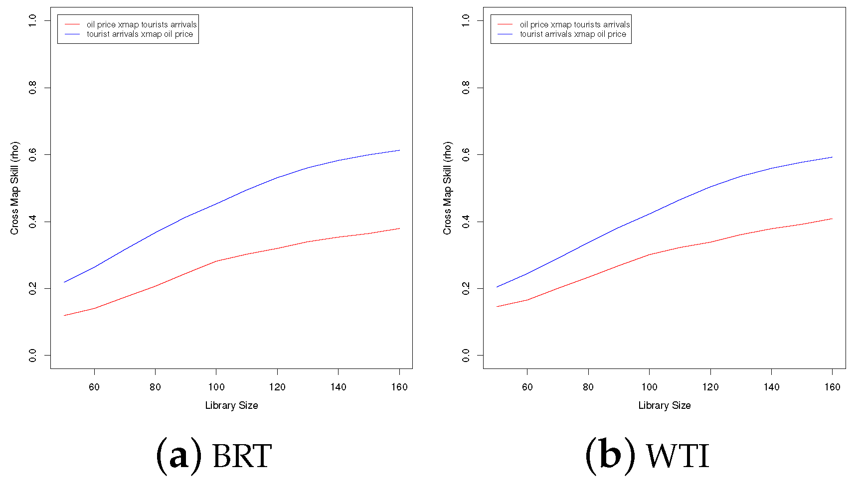
In this subsection, we present the findings following the initial application of CCM for the causality detection in oil–tourism studies, where tourist arrivals and oil prices in the US and nine European countries were taken into consideration. Given the nonparametric nature of the CCM technique, we made no prior linear model assumptions so to seek better understanding of the causal relationships in this complex, dynamical system. Note that all of the test results were obtained using the optimal embedding dimensions. More specifically, it was determined by the nearest neighbor forecasting performance using simplex projection; the library size ranges were identical to allow further comparisons; and leave-one-out cross validation was applied to determine the best choice of library size with optimal performance. The results of CCM tests between tourist arrivals and oil prices are briefly summarized in Table 5, and the details of the test results by country and type of oil price are listed in Appendix B.
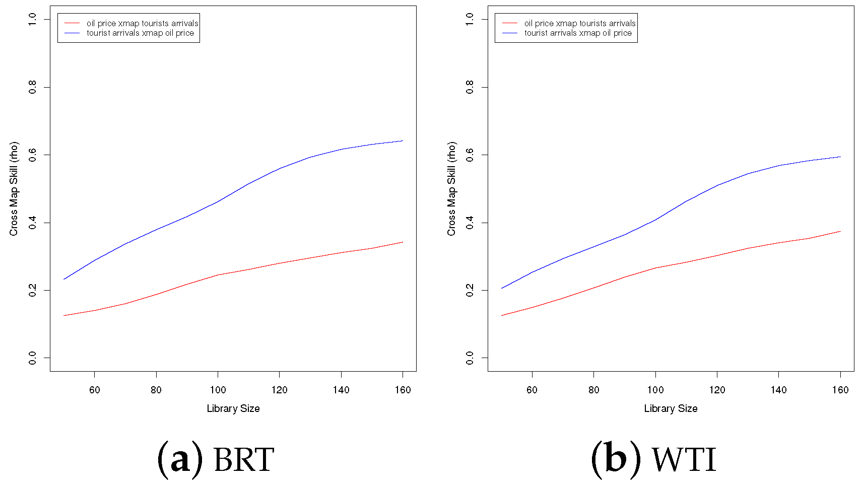
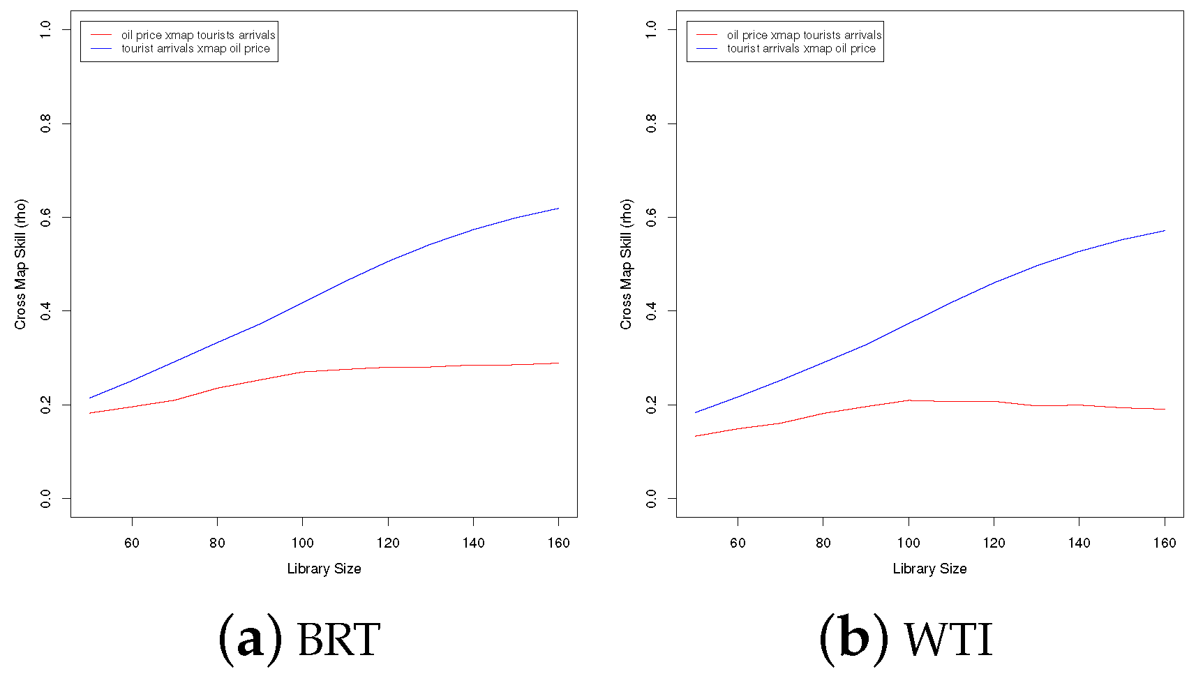
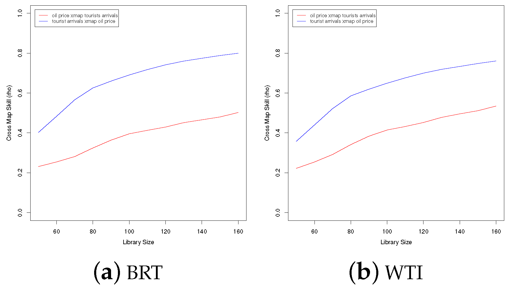
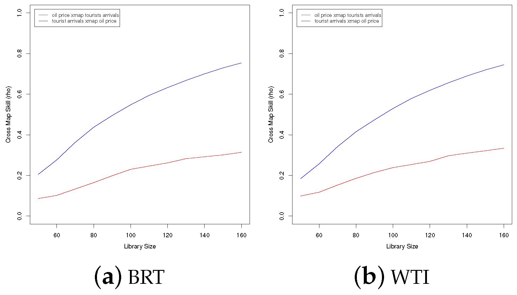
We found that significant causality was proven in general for all countries, as the test results strongly reflected a one-directional causal link from oil price to tourist arrivals. The results for BRT and WTI were very similar. For most of the countries, the cross map skill of oil price on tourist arrivals was also relatively high (still lower than the cross map skill in the opposite direction). These results not only reflect the close relationship between the two variables, regardless of the direction, but also confirm the findings of the established literature. Note that the improving trend in line with the increasing size of the library is reasonable as more data were used for cross validation in the cross map evaluation. The cross map skill from tourist arrivals to oil price (effect factor on cause factor) was much higher with a significant gap in between, representing the level of causation from oil price on tourist arrivals. A greater gap represents a stronger causality. Austria showed the most significant causality of tourist arrivals on oil prices, whilst the UK and US showed slightly less significant outcomes on average. In general, the CCM results proved a one-directional causal link from oil price to tourist arrivals for the US and the nine European countries.
As an advanced nonparametric causality detection method, CCM outperforms the empirical methods with its sensitiveness and ability to accurately detect causality when faced with a complex system and less amount of data. More importantly, the tests in the current study showed its significant ability to detect nonlinear causality and strong performance in identifying complex causal links in dynamical system. The results also indicated that CCM is a viable alternative for causality detection in the tourism industry.

6. Conclusions

This paper began with the aim of investigating the causality between the oil price and tourist arrivals in the US and nine European countries. Both empirical and novel methods of causality detection were conducted to contribute towards explaining the impacts of oil price volatility on tourist arrivals across countries. More specifically, the advanced nonparametric causality technique CCM proved the existence of one-directional causality from oil prices to tourist arrivals for all countries when the empirical methods all failed to detect the same.
This paper is also the first attempt at conducting a CCM causality detection in oil–tourism studies. The consistent and significant evidence presented herewith in terms of identifying significantly causal links across countries showed CCM to be a reliable and efficient method for causality detection when faced with complex and nonlinear scenarios, as witnessed in oil–tourism studies. We believe that the findings of this research will motivate further research in relation to the development and increased application of CCM in tourism studies where the multivariate analysis of complex systems can be of utmost importance.
As the initial attempt to adopt advanced techniques for the causality analysis between oil price and tourist arrivals, this paper established consistent evidence across countries. By providing a better understanding of the impacts of the oil price on tourist arrivals, we hope to contribute to the development of easy, efficient, data-driven, and robust techniques for causality analyses of nonlinear and complex systems whilst assisting policy making in terms of oil price volatility and economical activities closely related to tourism. This will assist countries and the tourism industry in managing the risks caused by oil price volatility, as well as making sufficient policy adjustments based on the oil–tourism dependence level that is easily comparable and efficiently presented by the method proposed in this paper. Considering the promising performance of CCM validated in this paper, this area of research expected to be extended further in future research by involving different types of tourists, tourism products, and destinations, etc. Moreover, research in progress is exploring the different components of data and their causality linkages via different approaches.

Author Contributions

Conceptualization, X.H., E.S. and H.H.; Investigation, X.H.; Methodology, X.H., E.S. and H.H.; Supervision, H.H.; Writing—review & editing, X.H., E.S. and H.H.

Funding

This research received no external funding.

Conflicts of Interest

The authors declare no conflict of interest.

Appendix A

Frequency domain causality test results (having greater test statistics (blue) than the corresponding 5% critical values (red) indicates possible causal links within the corresponding frequency range. Also, the optimal lag-structures were maintained for all tests).
Figure A1. Frequency causality results for tourist arrivals and oil prices in Austria.
Stats 01 00010 g0a1
Figure A2. Frequency causality results for tourist arrivals and oil prices in Germany.
Stats 01 00010 g0a2
Figure A3. Frequency causality results tourist arrivals and oil prices in Greece.
Stats 01 00010 g0a3
Figure A4. Frequency causality results for tourist arrivals and oil prices in Italy.
Stats 01 00010 g0a4
Figure A5. Frequency causality results for tourist arrivals and oil prices in the Netherlands.
Stats 01 00010 g0a5
Figure A6. Frequency causality results for tourist arrivals and oil prices in Portugal.
Stats 01 00010 g0a6
Figure A7. Frequency causality results for tourist arrivals and oil prices in Spain.
Stats 01 00010 g0a7
Figure A8. Frequency causality results for tourist arrivals and oil prices in Sweden.
Stats 01 00010 g0a8
Figure A9. Frequency causality results for tourist arrivals and oil prices in the UK.
Stats 01 00010 g0a9
Figure A10. Frequency causality results for tourist arrivals and oil prices in the US.
Stats 01 00010 g0a10

Appendix B

Convergent Cross Mapping test results (the cross map skill index reflects the reconstruction ability of the fact factor to the cause factor in both directions. Here, more specifically, the blue line above red line represents a significant cross map skill of tourist arrivals on oil price, which indicates causality from oil price to tourist arrivals. All tests were obtained with the optimal embedding dimensions; the results are presented as the optimal outcome based on the cross validation results).
Figure A11. CCM causality results for tourist arrivals and oil prices in Austria.
Stats 01 00010 g0a11
Figure A12. CCM causality results for tourist arrivals and oil prices in Germany.
Stats 01 00010 g0a12
Figure A13. CCM causality results for tourist arrivals and oil prices in Greece.
Stats 01 00010 g0a13
Figure A14. CCM causality results for tourist arrivals and oil prices in Italy.
Stats 01 00010 g0a14
Figure A15. CCM causality results for tourists arrival and oil prices in the Netherlands.
Stats 01 00010 g0a15
Figure A16. CCM causality results for tourist arrivals and oil prices in Portugal.
Stats 01 00010 g0a16
Figure A17. CCM causality results for tourist arrivals and oil prices in Spain.
Stats 01 00010 g0a17
Figure A18. CCM causality results for tourist arrivals and oil prices in Sweden.
Stats 01 00010 g0a18
Figure A19. CCM causality results for tourist arrivals and oil prices in the UK.
Stats 01 00010 g0a19
Figure A20. CCM causality results for tourist arrivals and oil prices in the US.
Stats 01 00010 g0a20

References

  1. Becken, S.; Lennox, J. Implications of a long-term increase in oil prices for tourism. Tour. Manag. 2012, 33, 133–142. [Google Scholar] [CrossRef]
  2. Becken, S. Developing indicators for managing tourism in the face of peak oil. Tour. Manag. 2008, 29, 695–705. [Google Scholar] [CrossRef]
  3. Chatziantoniou, I.; Filis, G.; Eeckels, B.; Apostolakis, A. Oil prices, tourism income and economic growth: A structural VAR approach for European Mediterranean countries. Tour. Manag. 2013, 36, 331–341. [Google Scholar] [CrossRef] [Green Version]
  4. Hamilton, J.D. This is what happened to the oil price-macroeconomy relationship. J. Monetary Econ. 1996, 38, 215–220. [Google Scholar] [CrossRef]
  5. Ferderer, J.P. Oil price volatility and the macroeconomy. J. Macroecon. 1997, 18, 1–26. [Google Scholar] [CrossRef]
  6. Sadorsky, P. Oil price shocks and stock market activity. Energy Econ. 1999, 21, 449–469. [Google Scholar] [CrossRef]
  7. Leduc, S.; Sill, K. A quantitative analysis of oil-price shocks, systematic monetary policy, and economic downturns. J. Monet. Econ. 2004, 51, 781–808. [Google Scholar] [Green Version]
  8. Huang, B.N.; Hwang, M.J.; Peng, H.P. The asymmetry of the impact of oil price shocks on economic activities: An application of the multivariate threshold model. Energy Econ. 2005, 27, 455–476. [Google Scholar] [CrossRef]
  9. Park, J.; Ratti, R.A. Oil price shocks and stock markets in the US and 13 European countries. Energy Econ. 2008, 30, 2587–2608. [Google Scholar] [CrossRef]
  10. Cong, R.G.; Wei, Y.M.; Jiao, J.L.; Fan, Y. Relationships between oil price shocks and stock market: An empirical analysis from China. Energy Policy 2008, 36, 3544–3553. [Google Scholar] [CrossRef]
  11. Hassani, H.; Zhigljavsky, A. Singular spectrum analysis: Methodology and application to economics data. J. Syst. Sci. Complex. 2009, 22, 372–394. [Google Scholar] [CrossRef]
  12. Ji, Q.; Fan, Y. How does oil price volatility affect non-energy commodity markets? Appl. Energy 2012, 89, 273–280. [Google Scholar] [CrossRef]
  13. Kilian, L.; Hicks, B. Did unexpectedly strong economic growth cause the oil price shock of 2003–2008? J. Forecast. 2013, 32, 385–394. [Google Scholar] [CrossRef]
  14. Acemoglu, D.; Finkelstein, A.; Notowidigdo, M.J. Income and health spending: Evidence from oil price shocks. Rev. Econ. Stat. 2013, 95, 1079–1095. [Google Scholar] [CrossRef]
  15. Wang, Y.; Wu, C.; Yang, L. Oil price shocks and stock market activities: Evidence from oil-importing and oil-exporting countries. J. Comp. Econ. 2013, 41, 1220–1239. [Google Scholar] [CrossRef]
  16. Yeoman, I.; Lennon, J.J.; Blake, A.; Galt, M.; Greenwood, C.; McMahon-Beattie, U. Oil depletion: What does this mean for Scottish tourism? Tour. Manag. 2007, 28, 1354–1365. [Google Scholar]
  17. Pentelow, L.; Scott, D. The implications of climate change mitigation policy and oil price volatility for tourism arrivals to the Caribbean. Tour. Hosp. Plan. Dev. 2010, 7, 301–315. [Google Scholar] [CrossRef]
  18. Tang, C.F. Temporal Granger Causality and the Dynamics Relationship Between RealTourism Receipts, Real Income and RealExchange Rates in Malaysia. Int. J. Tour. Res. 2013, 15, 272–284. [Google Scholar] [CrossRef]
  19. Goh, C. Exploring impact of climate on tourism demand. Ann. Tour. Res. 2012, 39, 1859–1883. [Google Scholar] [CrossRef]
  20. Sheldon, P.J.; Var, T. Tourism forecasting: A review of empirical research. J. Forecast. 1985, 4, 183–195. [Google Scholar]
  21. Chou, C.-M.; Hsieh, S.F.; Tseng, H.P. The crowding-out effects of Chinese tourists on inbound tourism in Taiwan. Tour. Econ. 2014, 20, 1235–1251. [Google Scholar] [CrossRef]
  22. Sugihara, G.; May, R.; Ye, H.; Hsieh, C.H.; Deyle, E.; Fogarty, M.; Munch, S. Detecting causality in complex ecosystems. Science 2012, 338, 496–500. [Google Scholar] [CrossRef] [PubMed]
  23. Song, H.; Li, G. Tourism demand modelling and forecasting: A review of recent research. Tour. Manag. 2008, 29, 203–220. [Google Scholar] [CrossRef] [Green Version]
  24. Gunter, U.; Onder, I. Forecasting international city tourism demand for Paris: Accuracy of uni- and multivariate models employing monthly data. Tour. Manag. 2015, 46, 123–135. [Google Scholar] [CrossRef]
  25. Becken, S. A critical review of tourism and oil. Ann. Tour. Res. 2011, 38, 359–379. [Google Scholar] [CrossRef]
  26. Selvanathan, S.; Selvanathan, E.A.; Viswanathan, B. Causality Between Foreign Direct Investment and Tourism: Empirical Evidence from India. Tour. Anal. 2012, 17, 91–98. [Google Scholar] [CrossRef]
  27. Massidda, C.; Mattana, P. A SVECM Analysis of the Relationship between International Tourism Arrivals, GDP and Trade in Italy. J. Travel Res. 2012, 52, 93–105. [Google Scholar] [CrossRef]
  28. Tang, C.F.; Tan, E.C. How stable is the tourism-led growth hypothesis in Malaysia? Evidence from disaggregated tourism markets. Tour. Manag. 2013, 37, 52–57. [Google Scholar] [CrossRef]
  29. Ghartey, E.E. Effects of tourism, economic growth, real exchange rate, structural changes and hurricanes in Jamaica. Tour. Econ. 2013, 19, 919–942. [Google Scholar] [CrossRef]
  30. Cellini, R.; Cuccia, T. Museum and monument attendance and tourism flow: A time series analysis approach. Appl. Econ. 2013, 45, 473–3482. [Google Scholar] [CrossRef] [Green Version]
  31. Albaladejo, I.P.; González-Martínez, M.I.; Martínez-García, M.P. Quality and endogenous tourism: An empirical approach. Tour. Manag. 2014, 41, 141–147. [Google Scholar] [CrossRef]
  32. Katircioğlu, S.T. Testing the tourism-induced EKC hypothesis: The case of Singapore. Econ. Model. 2014, 41, 383–391. [Google Scholar] [CrossRef]
  33. Katircioğlu, S.T.; Feridun, M.; Kilinc, C. Estimating tourism-induced energy consumption and CO2 emissions: The case of Cyprus. Renew. Sustain. Energy Rev. 2014, 29, 634–640. [Google Scholar] [CrossRef]
  34. Tang, C.F.; Abosedra, S. Small sample evidence on the tourism-led growth hypothesis in Lebanon. Curr. Issues Tour. 2014, 17, 234–246. [Google Scholar] [CrossRef]
  35. Fereidouni, H.G.; Al-mulali, U. The interaction between tourism and FDI in real estate in OECD countries. Curr. Issues Tour. 2014, 17, 105–113. [Google Scholar] [CrossRef]
  36. Solarin, S.A. Tourist arrivals and macroeconomic determinants of CO2 emissions in Malaysia. Anatolia 2014, 25, 228–241. [Google Scholar] [CrossRef]
  37. Antonakakis, N.; Dragouni, M.; Filis, G. Tourism and growth: The times they are a-changing. Ann. Tour. Res. 2015, 50, 165–169. [Google Scholar] [CrossRef] [Green Version]
  38. Chen, M.-H.; Lin, C.-P.; Chen, B.T. Drivers of Taiwan’s Tourism Market Cycle. J. Travel Tour. Mark. 2015, 32, 260–275. [Google Scholar] [CrossRef]
  39. Tang, C.F.; Tan, E.C. Does tourism effectively stimulate Malaysia’s economic growth? Tour. Manag. 2015, 46, 158–163. [Google Scholar] [CrossRef]
  40. Paerez-Rodríguez, J.V.; Ledesma-Rodríguez, F.; Santana-Gallego, M. Testing dependence between GDP and tourism’s growth rates. Tour. Manag. 2015, 48, 268–282. [Google Scholar] [CrossRef]
  41. Antonakakis, N.; Dragouni, M.; Filis, G. How strong is the linkage between tourism and economic growth in Europe? Econ. Model. 2015, 44, 142–145. [Google Scholar] [CrossRef] [Green Version]
  42. Dogan, E.; Seker, F.; Bulbul, S. Investigating the impacts of energy consumption, real GDP, tourism and trade on CO2 emissions by accounting for cross-sectional dependence: A panel study of OECD countries. Curr. Issues Tour. 2015, 20, 1701–1719. [Google Scholar] [CrossRef]
  43. Shahbaz, M.; Kumar, R.R.; Ivanov, S.; Loganathan, N. The nexus between tourism demand and output per capita, with the relative importance of trade openness and financial development: A study of Malaysia. Tour. Econ. 2015, 23, 168–186. [Google Scholar] [CrossRef]
  44. Al-Mulali, U.; Fereidouni, H.G.; Mohammed, A.H. The effect of tourism arrival on CO2 emissions from transportation sector. Anatolia 2015, 26, 230–243. [Google Scholar] [CrossRef]
  45. Durbarry, R.; Seetanah, B. The Impact of Long Haul Destinations on Carbon Emissions: The Case of Mauritius. J. Hosp. Mark. Manag. 2015, 24, 401–410. [Google Scholar] [CrossRef]
  46. Ertugrul, H.M.; Mangir, F. The tourism-led growth hypothesis: Empirical evidence from Turkey. Curr. Issues Tour. 2015, 18, 633–646. [Google Scholar] [CrossRef]
  47. Tang, C.F.; Tan, E.C. Tourism-Led Growth Hypothesis in Malaysia: Evidence Based Upon Regime Shift Cointegration and Time-Varying Granger Causality Techniques. Asia-Pac. J. Tour. Res. 2015, 20, 1430–1450. [Google Scholar] [CrossRef]
  48. Tsui, W.H.K.; Fung, M.K.Y. Causality between business travel and trade volumes: Empirical evidence from Hong Kong. Tour. Manag. 2016, 52, 395–404. [Google Scholar] [CrossRef]
  49. Zaman, K.; Shahbaz, M.; Loganathan, N.; Raza, S.Y. Tourism development, energy consumption and Environmental Kuznets Curve: Trivariate analysis in the panel of developed and developing countries. Tour. Manag. 2016, 54, 275–283. [Google Scholar] [CrossRef]
  50. Rakotondramaro, H.; Andriamasy, L. Multivariate Granger Causality among tourism, poverty and growth in Madagascar. Tour. Manag. Perspect. 2016, 20, 109–111. [Google Scholar] [CrossRef]
  51. Tang, C.F.; Abosedra, S. Tourism and growth in Lebanon: New evidence from bootstrap simulation and rolling causality approaches. Empir. Econ. 2016, 50, 679–696. [Google Scholar] [CrossRef]
  52. Toda, H.Y.; Yamamoto, T. Statistical inference in vector autoregressions with possibly integrated processes. J. Econom. 1995, 66, 225–250. [Google Scholar] [CrossRef]
  53. Dolado, J.J.; Lütkepohl, H. Making Wald tests work for cointegrated VAR system. Econom. Rev. 1996, 15, 369–386. [Google Scholar] [CrossRef]
  54. Zhang, H.Q.; Kulendran, N. The Impact of Climate Variables on Seasonal Variation in Hong Kong Inbound Tourism Demand. J. Travel Res. 2016, 26, 94–107. [Google Scholar] [CrossRef]
  55. Hatemi-J, A. On the tourism-led growth hypothesis in the UAE: A bootstrap approach with leveraged adjustments. Appl. Econ. Lett. 2016, 23, 424–427. [Google Scholar] [CrossRef]
  56. Li, X.; Pan, B.; Law, R.; Huang, X. Forecasting tourism demand with composite search index. Tour. Manag. 2017, 59, 57–66. [Google Scholar] [CrossRef]
  57. Valadkhani, A.; Smyth, R.; O’Mahony, B. Asymmetric causality between Australian inbound and outbound tourism flows. Appl. Econ. 2017, 49, 33–50. [Google Scholar] [CrossRef]
  58. Granger, C.W. Investigating causal relations by econometric models and cross-spectral methods. Econ. J. Econ. Soc. 1969, 37, 424–438. [Google Scholar] [CrossRef]
  59. Sims, C.A. Money, income, and causality. Am. Econ. Rev. 1972, 62, 540–552. [Google Scholar]
  60. Hsiao, C. Autoregressive modelling and money-income causality detection. J. Monetary Econ. 1981, 7, 85–106. [Google Scholar] [CrossRef]
  61. Sims, C.A.; Stock, J.H.; Watson, M.W. Inference in linear time series models with some unit roots. Econ. J. Econ. Soc. 1990, 58, 113–144. [Google Scholar] [CrossRef]
  62. Toda, H.Y.; Phillips, P.C. Vector autoregressions and causality. Econ. J. Econ. Soc. 1993, 61, 1367–1393. [Google Scholar] [CrossRef]
  63. Pesaran, H.H.; Shin, Y. Generalized impulse response analysis in linear multivariate models. Econ. Lett. 1998, 58, 17–29. [Google Scholar] [CrossRef] [Green Version]
  64. Chen, Y.; Bressler, S.L.; Ding, M. Frequency decomposition of conditional Granger causality and application to multivariate neural field potential data. J. Neurosci. Methods 2006, 150, 228–237. [Google Scholar] [CrossRef] [PubMed] [Green Version]
  65. Gow, D.W.; Segawa, J.A.; Ahlfors, S.P.; Lin, F.H. Lexical influences on speech perception: A Granger causality analysis of MEG and EEG source estimates. Neuroimage 2008, 43, 614–623. [Google Scholar] [CrossRef] [PubMed] [Green Version]
  66. Deshpande, G.; Sathian, K.; Hu, X. Effect of hemodynamic variability on Granger causality analysis of fMRI. Neuroimage 2010, 52, 884–896. [Google Scholar] [CrossRef] [PubMed] [Green Version]
  67. Geweke, J. Measurement of linear dependence and feedback between multiple time series. J. Am. Stat. Assoc. 1982, 77, 304–324. [Google Scholar] [CrossRef]
  68. Ciner, C. Eurocurrency interest rate linkages: A frequency domain analysis. Rev. Econ. Financ. 2011, 20, 498–505. [Google Scholar] [CrossRef]
  69. Breitung, J.; Candelon, B. Testing for short- and long-run causality: A frequency-domain approach. J. Econom. 2006, 132, 363–378. [Google Scholar] [CrossRef]
  70. Deyle, E.; Fogarty, M.; Hsieh, C.; Kaufman, L.; MacCall, A.; Munch, S.; Perretti, C.; Ye, H.; Sugihara, G. Predicting climate effects on Pacific sardine. Proc. Natl. Acad. Sci. USA 2013, 110, 6430–6435. [Google Scholar] [CrossRef] [PubMed]
  71. Ye, H.; Deyle, E.; Gilarranz, L.; Sugihara, G. Distinguishing time-delayed causal interactions using convergent cross mapping. Sci. Rep. 2015, 5, 14750. [Google Scholar] [CrossRef] [PubMed] [Green Version]
  72. Clark, A.T.; Ye, H.; Isbell, F.; Deyle, E.; Cowles, J.; Tilman, G.; Sugihara, G. Spatial convergent cross mapping to detect causal relationships from short time series. Ecology 2015, 96, 1174–1181. [Google Scholar] [CrossRef] [PubMed]
  73. Sugihara, G.; May, R. Nonlinear forecasting as a way of distinguishing chaos from measurement error in time series. Nature 1990, 344, 734–741. [Google Scholar] [CrossRef] [PubMed]
  74. Takens, F. Detecting strange attractors in turbulence Dynamical Systems and Turbulence. Dyn. Syst. Turbul. 1981, 898, 366–381. [Google Scholar]
  75. EIA. U.S. Energy Information Administration. 2016. Available online: http://www.eia.gov/outlooks/steo/outlook.cfm (accessed on 15 December 2016).
  76. Hassani, H.; Mahmoudvand, R.; Omer, H.N.; Silva, E.S. A Preliminary Investigation into the Effect of Outlier(s) on Singular Spectrum Analysis. Fluct. Noise Lett. 2014, 13, 1450029. [Google Scholar] [CrossRef]
  77. Akaike, H. Maximum likelihood identification of Gaussian autoregressive moving average models. Biometrika 1973, 60, 255–265. [Google Scholar] [CrossRef]
  78. Schwarz, G. Estimating the dimension of a model. Ann. Stat. 1978, 6, 461–464. [Google Scholar] [CrossRef]
  79. Hannan, E.J.; Quinn, B.G. The determination of the order of an autoregression. J. R. Stat. Soc. Ser. B-Stat. Methodol. 1979, 42, 190–195. [Google Scholar]
  80. Akaike, H. Fitting autoregressive models for prediction. Ann. Inst. Stat. Math. 1969, 21, 243–247. [Google Scholar] [CrossRef]
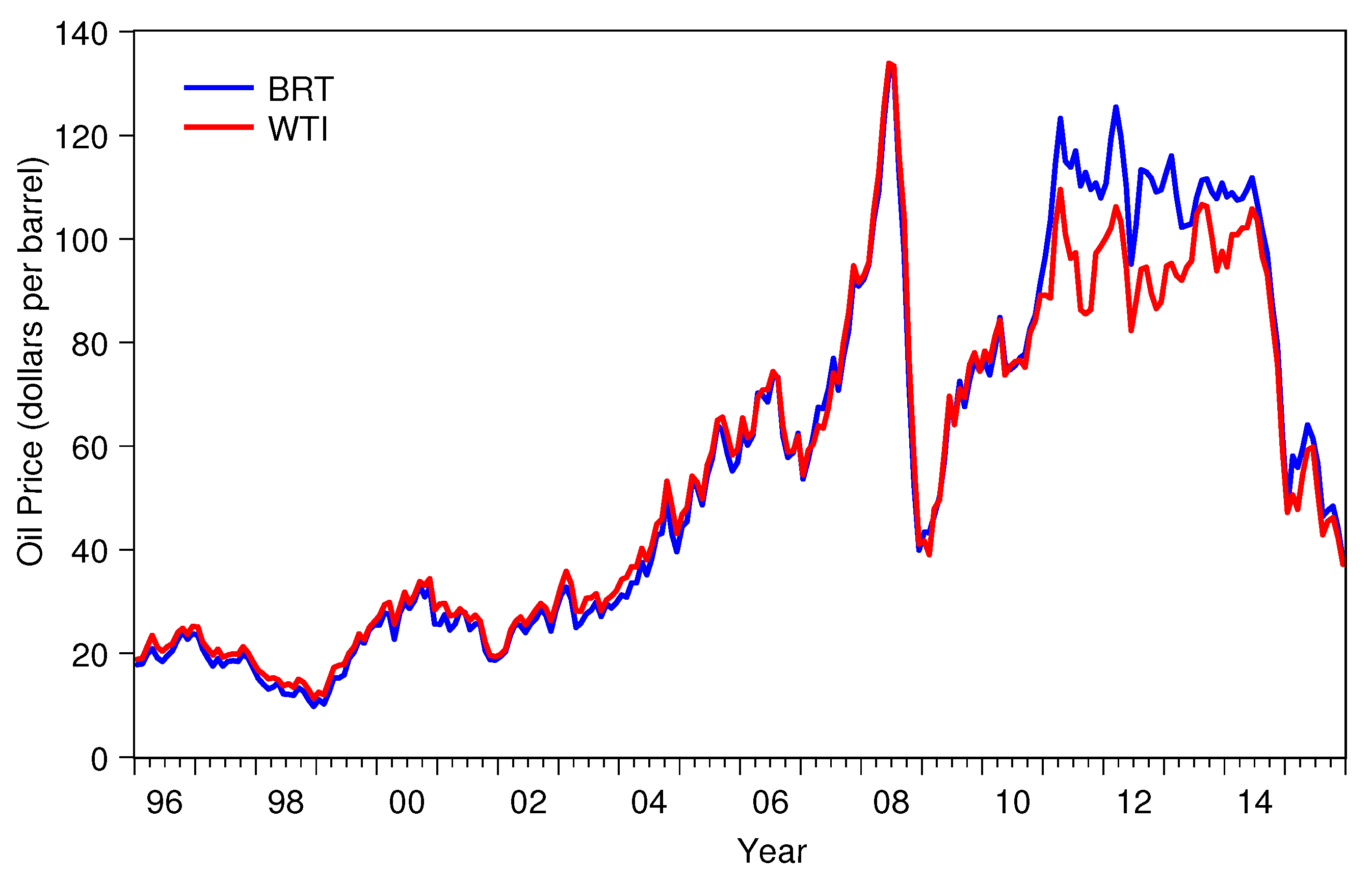
Figure 1. Monthly oil price data from 1996 to 2015.
Stats 01 00010 g001
Figure 2. Monthly tourist arrivals data from 1996 to 2015 by country.
Stats 01 00010 g002
Table 1. Descriptive statistics for the data.
Oil Prices
ObsMeanMedianMaxMinSDSkewnessKurtosis
BRT24056.4149.22132.729.8235.240.471.85
WTI24054.7849.06133.8811.3531.190.401.89
Tourist Arrivals
ObsMeanMedianMaxMinStd. Dev.SkewnessKurtosis
Austria2401,481,8941,434,4553,205,966446,240504,4480.393.21
Germany2401,918,3941,788,5834,401,682747,141724,5520.753.29
Greece240765,847564,5233,107,95529,856710,6111.113.66
Italy2403,343,9533,277,0848,084,209907,3671,709,1180.502.45
Netherland240870,900864,2001,745,779275,000284,1800.342.79
Portugal240539,796522,3951,359,284155,438256,2800.703.03
Spain2403,229,3142,934,3737,443,749671,1091,533,2090.512.42
Sweden240357,927239,9021,428,20798,357289,0811.935.97
UK2401,668,0201,541,0003,390,515692,120582,2390.592.64
US2404,325,3744,222,0348,364,9402,094,2871,292,7870.592.88
Note: Obs—Number of Observations; Max—Maximum Value; Min—Minimum Value; SD—Standard Deviation.
Table 2. Unit root test results.
VariablesSeriesMethodsNoneInterceptIntercept and Trend
LevelDecisionLevelDecisionLevelDecision
Oil Prices
(240 Obs)
January 1996–December 2015
BRTKPSS------------------1.675 ***(11)I(1)0.139 *(11)I(0)
ADF−10.284 ***(0)I(1)−10.264 ***(0)I(1)−10.294 ***(0)I(1)
PP−10.279 ***(4)I(1)−10.258 ***(4)I(1)−10.283 ***(4)I(1)
WTIKPSS------------------1.663 ***(11)I(1)0.166 **(11)I(1)
ADF−10.104 ***(0)I(1)−10.083 ***(0)I(1)−10.109 ***(0)I(1)
PP−10.104 ***(0)I(1)−10.083 ***(0)I(1)−10.109 ***(0)I(1)
Tourist Arrivals
(240 Obs)
January 1996–December 2015
AustriaKPSS------------------1.458 ***(15)I(1)0.144 *(27)I(0)
ADF−3.938 ***(14)I(1)−16.637 ***(11)I(1)−17.093 ***(11)I(0)
PP−49.801 ***(23)I(1)−9.945 ***(31)I(0)−10.345 ***(24)I(0)
GermanyKPSS------------------2.305 ***(9)I(1)0.115(1)I(0)
ADF−2.524 ***(13)I(1)−3.581 ***(13)I(1)−3.825 ***(13)I(1)
PP−12.185 ***(16)I(1)−4.832 ***(5)I(0)−5.169 ***(0)I(0)
GreeceKPSS------------------0.755 ***(3)I(1)0.058(2)I(0)
ADF−4.411 ***(11)I(1)−4.791 ***(11)I(1)−4.985 ***(11)I(1)
PP−4.056 ***(5)I(0)−5.414 ***(6)I(0)−5.529 ***(6)I(0)
ItalyKPSS------------------1.079 ***(5)I(1)0.014(2)I(0)
ADF−3.527 ***(13)I(1)−4.403 ***(13)I(1)−4.527 ***(13)I(1)
PP−2.828 ***(3)I(0)−6.291 ***(4)I(0)−6.604 ***(4)I(0)
NetherlandKPSS------------------1.744 ***(8)I(1)0.084(4)I(0)
ADF−2.976 ***(13)I(1)−3.496 ***(13)I(1)−3.503 ***(13)I(1)
PP−14.361 ***(3)I(1)−5.952 ***(2)I(0)−6.548 ***(1)I(0)
PortugalKPSS------------------1.653 ***(7)I(1)0.111(1)I(0)
ADF−4.077 ***(12)I(1)−4.658 ***(12)I(1)−4.848 ***(12)I(1)
PP−2.101 **(6)I(0)−5.731 ***(5)I(0)−5.672 ***(6)I(0)
SpainKPSS------------------1.991 ***(8)I(1)0.071(1)I(0)
ADF−2.353 **(12)I(1)−2.857 *(12)I(0)−3.469 **(13)I(0)
PP−2.306 **(4)I(0)−5.646 ***(4)I(0)−6.118 ***(5)I(0)
SwedenKPSS------------------1.052 ***(2)I(1)0.161 **(9)I(1)
ADF−5.708 ***(13)I(1)−6.117 ***(13)I(1)−6.104 ***(13)I(1)
PP−3.940 ***(14)I(0)−5.961 ***(19)I(0)−5.794 ***(24)I(0)
UKKPSS------------------0.818 ***(5)I(1)0.090(3)I(0)
ADF−4.889 ***(12)I(1)−4.981 ***(12)I(1)−5.196 ***(12)I(1)
PP−10.446 ***(4)I(1)−5.821 ***(1)I(0)−6.387 ***(2)I(0)
USKPSS------------------1.825 ***(11)I(1)0.392 ***(9)I(1)
ADF−3.591 ***(12)I(1)−3.928 ***(12)I(1)−4.074 ***(12)I(1)
PP−19.331 ***(6)I(1)−3.796 ***(8)I(0)−7.063 ***(8)I(0)
a *, **, and *** indicate significance at the 10%, 5%, and 1% levels respectively. b The critical values were as follows: (1) none: −2.574, −1.942, and −1.616 for augmented Dickey–Fuller (ADF) and Phillips and Perron (PP) at the 1%, 5%, and 10% levels of significance, respectively; (2) intercept: −3.457, −2.873, and −2.573 {0.739, 0.463, 0.347} for ADF and PP {KPSS} at the 1%, 5%, and 10% levels of significance, respectively; (3) intercept and trend: −3.996, −3.428, and −3.137 {0.216, 0.146, 0.119} for ADF and PP{KPSS} at the 1%, 5%, and 10% levels of significance, respectively. c The numbers in parentheses for the ADF and PP tests indicate lag-lengths selected based on the Schwarz Information Criterion (SIC). For the Kwiatkowski–Phillips–Schmidt–Shin (KPSS) test, based on the Bartlett kernel spectral estimation method, the corresponding numbers represent the Newey–West bandwidth.
Table 3. Time domain Granger causality test results.
CountryOil Prices
BRTWTI
p-ValueYes/Nop-ValueYes/Nop-ValueYes/Nop-ValueYes/No
Austria0.68No0.56No0.81No0.34No
Germany0.52No0.27No0.29No0.17No
Greece0.54No0.36No0.46No0.44No
Italy0.60No0.98No0.67No0.74No
Netherlands0.30No0.83No0.29No0.65No
Portugal0.38No0.41No0.72No0.31No
Spain0.62No0.24No0.54No0.12No
Sweden0.21No0.55No0.14No0.93No
UK0.63No0.95No0.53No0.82No
US0.48No0.85No0.53No0.48No
Notes: → indicates tourist arrivals causes oil price; ← indicates oil price causes tourist arrivals.
Table 4. Frequency domain causality test results.
CountryOil Prices
BRTWTI
AustriaNoNoNoNo
GermanyNoNoNoNo
GreeceNoNoNoNo
ItalyNoNoNoNo
NetherlandNoNoNoNo
PortugalNoNoNoNo
SpainNoNoNoNo
SwedenNoNoNoNo
UKNoNoNoNo
USNoNoNoNo
Notes: → indicates tourist arrivals causes oil price; ← indicates oil price causes tourist arrivals.
Table 5. Convergent Cross Mapping (CCM) causality test results.
CountryOil Prices
BRTWTI
AustriaNoYesNoYes
GermanyNoYesNoYes
GreeceNoYesNoYes
ItalyNoYesNoYes
NetherlandNoYesNoYes
PortugalNoYesNoYes
SpainNoYesNoYes
SwedenNoYesNoYes
UKNoYesNoYes
USNoYesNoYes
Notes: → indicates tourist arrivals causes oil price; ← ndicates oil price causes tourist arrivals.