Abstract
We investigated the influence of natural and anthropogenic sources on bulk atmospheric deposition chemistry, from November 2017 until October 2019, in a Brazilian agricultural area. The pH mean value was 5.99 (5.52–8.46) and most deposition samples (~98%) were alkaline (pH > 5.60). We identified Ca2+ as the predominant species, accounting for 33% of the total ionic species distribution and the main precursor of atmospheric acidity neutralization (Neutralization Factor = 6.63). PMF analysis resulted in four factors, which demonstrated the influence of anthropogenic and natural sources, such as fertilizer application and production, marine intrusion/biomass burning, and biogenic emissions, and revealed the importance of atmospheric neutralization processes.
1. Introduction
Because of rapid economic development, increased energy consumption, anthropogenic activities, and industrialization over the last centuries, the atmospheric accumulation of several gases and aerosols was inevitable []. These pollutants move from the atmosphere to Earth’s surface mainly by bulk deposition processes, which encompasses wet (in-cloud and below-cloud scavenging processes) and dry deposition (scavenging processes in the absence of precipitation) []. Therefore, owing to atmospheric deposition, nutrients and pollutants may entry into terrestrial and aquatic ecosystems causing significant impacts, such as eutrophication and soil acidity [].
Atmospheric deposition chemistry has been widely studied in many areas worldwide and provides useful information that feeds several receptor models to identify anthropogenic and natural source apportionment [,,,]. Broadly, natural origin is related to marine salt and soil dust, while anthropogenic origins are mainly fossil fuel combustion, industrial processes, and agricultural production []. Moreda-Piñeiro et al. [] assessed rainwater samples in Spain and reported that Cl−, Na+, and Mg2+ were linked to sea salt, while SO42− and Ca2+ were released from a terrestrial crustal source. Also, in this study, NH4+ and NO3− were mainly attributed to agricultural activity.
Statistical techniques, such as Factor Analysis (FA), Principal Component Analysis (PCA), Chemical Mass Balance (CMB), and Positive Matrix Factorization (PMF), have been employed as receptor models for the identification of the main sources of pollutants [,,]. However, PMF is commonly applied to airborne particles and atmospheric gases [,] and rarely to bulk atmospheric deposition due to the complexity of its process [].
Considering the absence of an established network for routinely monitoring wet and dry deposition in Brazil [], a study was carried out in the Southern region of Minas Gerais, which is an important economic region responsible for 21.8% of agricultural commodities (mainly from coffee-producing regions), and also accounts for about 12% of the state’s Gross Domestic Product []. We investigated the influence of natural and anthropogenic sources on bulk atmospheric deposition chemistry in Lavras, a city in Southern Minas Gerais, using PMF.
2. Material and Methods
2.1. Study Area
Lavras is located in the Southern Minas Gerais state (21°13′45.3″ S and 44°58′32.4″ W), Brazil, 241 km from the Atlantic Ocean (in a straight line), with an area of 564.744 km2, altitude of 919 m (Figure 1) and a population of 102,728 inhabitants []. Lavras’ soil is predominantly classified as Dystrophic Red-Yellow Oxisol (RYOd1) and Eutrophic Red-Yellow Argisol (RYAe12). RYOd1 soils are suitable for tillage but are naturally acidic []. Therefore, the liming process is common, in which lime is applied to correct soil acidity for agricultural purposes. Lavras is generally known for its agricultural production since about 19% (107 km2) of its total area is associated with agricultural activities, mainly coffee production [].
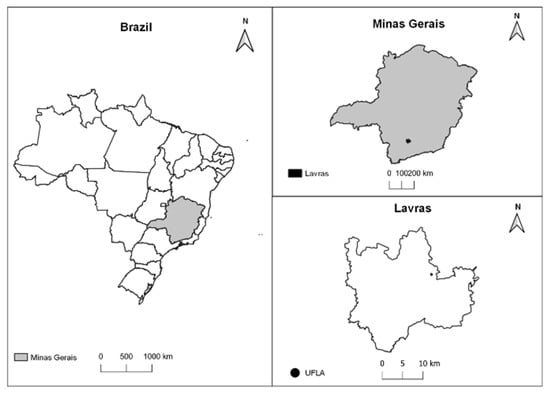
Figure 1.
Geographical location of sampling site (UFLA) in Lavras, Southern Minas Gerais state, Brazil.
Lavras is also influenced by several anthropogenic activities, including transport, farming, biomass burning, and industrial activities such as agroindustrial, limestone mining, and cement manufacturing []. The vehicular fleet has about 50 thousand light-duty vehicles, of which 54% are automobiles and 26% are motorcycles. Moreover, the vehicle fleet is, on average, 15 years old, where 62% of passenger cars were produced before 2010 and 14% before 1990 [].
Regarding weather conditions, the city has a mean annual (1981–2010) temperature of 20.3 °C, with minimum (16.9 °C) values in July and maximum (22.8 °C) in February. The annual rainfall of 1461.8 mm is mainly concentrated in two well-defined periods: (i) a rainy season from October to March (covering 85% of total rainfall), and (ii) a dry one from April to September [].
2.2. Sampling and Sample Analysis
A total of 65 bulk deposition samples were collected at Universidade Federal de Lavras (UFLA) campus in Lavras (Figure 1) between November 2017 and October 2019 using a handmade sampler composed of a high-density polyethylene bucket (NALGON) of 10 L with a collecting area of 439 cm2, protected by a sun-protective PVC structure and covered with a nylon mesh. In order to follow GAW’s sampling procedures, the sampler was kept 1.5 m above the ground and cleaned with deionized water (18 MΩ) []. It should be noted that for dry atmospheric only samples, 50 mL of deionized water was added in order to analyze soluble species.
Samples were collected at intervals of about seven days, and after each collection, they were divided into two parts. In a fraction of the samples, pH was measured using a pH meter (AKSO AK model 151), calibrated with buffer solutions (pH 4.0 and 7.0). The other sample aliquot was filtered with a 0.22 μm diameter membrane (Millex), stored in pre-cleaned polyethylene bottles kept at −18 °C prior to ion chromatography (IC) analysis (Metrohm model 851) with anionic column (Metrosep ASupp 5–250 mm × 4 mm) and cationic column (Metrosep C2 150–150 × 4 mm). Analytical quantification was performed using an external calibration curve from the standard concentrations for each ion. The specıes quantıfıed by IC were calcium (Ca2+), ammonium (NH4+), magnesium (Mg2+), sodium (Na+), potassium (K+), nitrate (NO3−), chloride (Cl−), sulfate (SO42−), fluoride (F−), formate (CHO2−), acetate (C2H3O2−), and oxalate (C2O42−), all presenting detection limits (DL) lower than 0.8 µmolL−1. Also, blank sample analyses were carried out through the sampling campaign.
2.3. Data Analysis
Data processing was performed by programming in R language, specifically the functions contained in the stats and ggplot2 packages [,].
2.3.1. Samples Validation
The internal consistency of the entire data set was analyzed through Cooperative Programme for Monitoring and Evaluation of Long-Range Transmission of Air Pollutants in Europe (EMEP) guidelines for rainwater sample validation []. This method is based on the Equations (1)–(3):
where Ci is the concentration of ion type i in a specific sample, expressed in µeqL−1. IS is the sum of all ion concentrations, and ID is the difference between the sum of the cation concentrations and the sum of the anion concentrations. Both IS and ID are expressed in µeqL−1. The ion balance, IB, expresses the difference, ID, in percent of the sum of all concentrations, IS. Apart from the equations, the samples’ pH values were also considered in this validation process; a critical value of 5.5 was used. Moreover, specific details are described elsewhere [,].
2.3.2. Non-Measure Species Estimate
We estimate bicarbonate (HCO3−) concentrations from the theoretical relationship between pH and HCO3− (Equation (4)), and for carbonate (CO32−), we considered the same concentration of Ca2+ [], since no direct method was applied for measuring these species.
2.3.3. Volume Weighted Mean
The volume-weighted mean (VWM) was expressed through the relationship between the sum of the concentrations product of each species (Xi) found in the n samples by the respective volume (Vi) and the sum of all the sample volumes according to Equation (5) []. For dry atmospheric deposition samples, in which we added 50 mL of deionized water due to precipitation absence, we considered that volume for calculations.
2.3.4. Neutralization Factor
The neutralization factor (NF) or index was calculated to assess the role of crustal components (Ca2+ and Mg2+) and NH4+ on the neutralization of rainwater acidity due to the presence of NO3− and SO42−, using Equation (6) adapted from Huang et al. and Qiao et al. [,]:
where X is the cation of interest and all the concentrations were used in µeqL−1.
2.3.5. Positive Matrix Factorization (PMF)
Sources of pollutants and their relative contributions were identified using Positive Matrix Factorization (PMF; version 5.0; US EPA Research, Durham, NC, USA) software made available by the United States Environmental Protection Agency, which consists of a mathematical receptor model []. The model software is available for free at https://www.epa.gov/air-research/positive-matrix-factorization-model-environmental-data-analyses (accessed on 9 September 2021).
In general, a receptor model aims to solve the chemical mass balance between the species’ measured concentrations and the sources profiles []. In this sense, the PMF model decomposes a matrix of sample data into one matrix of factor contributions (G) and another of factor profiles (F). Then, for a data matrix X of n samples by m chemical species, the model will identify the number of factors p, the species profile fk of each factor k, and the amount of mass gk contributed by each factor k to each individual sample, according to Equation (7):
where eij is the residual, i and j are the rows and columns of X.
The factor contributions and profiles are derived by the PMF model minimizing the Q function (Equation (8)), with non-negativity constraints, i.e., gik > 0 and fkj > 0 [,].
where uij are variable uncertainties, which allowing each data value to be individually weighted. These variable uncertainties (uij) for data with values below and above the DL were calculated according to Equations (9) and (10), respectively [,].
where the error fraction was estimated at 10% [].
The quality of data was assessed based on the signal-to-noise ratio (S/N), which characterize species as strong when S/N > 2.0 and as weak in the cases that S/N ranged from 0.2 to 2.0. Species with S/N < 0.2 or values below DL greater than 50% were categorized as bad in quality and were excluded from the PMF analysis [].
3. Results and Discussion
3.1. Samples Validation
The pH values for the whole data set (n = 65) ranged from 5.34 to 8.46, with an average of 5.89. Given the samples’ alkaline behavior, quality assurance and quality control (QA/QC) were verified applying the criteria from EMEP. Following the QA/QC, among the 65 atmospheric deposition events, 7 were invalid, 3 were valid, and 55 were valid and flagged (Figure 2a). Only seven invalid samples were rejected, and, therefore, we considered a new data set (n = 58) in the following discussion.
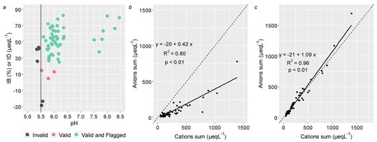
Figure 2.
Ionic balance in bulk atmospheric deposition of Lavras: (a) samples validation criteria from EMEP (n = 66) and the reference line represent a critical pH (5.5) value; (b) anions sum vs. cations sum (n = 58) and the dashed line represent the ideal slope of 1; (c) anions sum vs. cations sum considering the carbonate estimate (n = 58) and the dashed line represent the ideal slope of 1. Sampling period was between November 2017 and October 2019.
In order to verify the electroneutrality principle, a sum of anions versus cations plot was depicted in Figure 2b, in units of µeqL−1. In general, we observed a good and statistically significant linear fit (R2 = 0.80 and p-value < 0.01) for the data set. In addition, the sum of cations was greater than the sum of anions since the fitted line slope (value of 0.42—Figure 2b) was lower than the unity. The anions deficit was reasonable in samples with pH values ranging from 5.5 to 6.0 [], which could have been attributed to the lack of measurements of carbonate and bicarbonate concentration [,,]. In order to identify the carbonate deficit, an estimative of these species was carried out (WMO, 2004), and a new sum of cations versus anions plot was constructed (Figure 2c). It is noteworthy that the new angular coefficient presented a value of 1.09, which was closer to 1, with a determination coefficient of 96% (p-value < 0.01). The bicarbonate estimation produced a poor linear adjustment (slope = 0.32 and R2 = 0.04 with p-value 0.07), and therefore, we considered only the presence of carbonate in the bulk atmospheric deposition samples.
3.2. pH Variation
The mean pH value for validated samples (n = 58) was 5.99 (5.52–8.46) (Figure 3). Once 5.60 represents the pH value resulting from the equilibrium between atmospheric CO2 and pure water and is also used as a limit for acid rain [,,], our results suggest inputs of alkaline species into the atmosphere (98% of samples with pH > 5.60). This behavior is in agreement with other studies carried out in Brazil, such as those performed in Campo Bom, Rio Grande do Sul [] and in Juiz de Fora, Minas Gerais [], in which the authors’ associated high pH values to inputs of crustal aerosols, containing large fractions of carbonate and bicarbonate, in the atmospheric deposition.
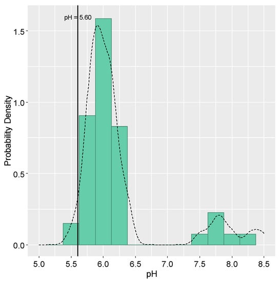
Figure 3.
Histogram of the pH values of the 58 bulk atmospheric deposition samples in Lavras, from November 2017 until October 2019. The vertical line refers to the critical value for rainwater acidity classification (pH = 5.60) and the dotted line represents the probability density curve.
3.3. Ionic Composition
The concentration of major ions in μmolL−1 is illustrated in Figure 4. Among all cations, Ca2+ was the specie with the greatest variability (6.82–455 μmolL−1), followed by Na2+ (0.03–179 μmolL−1). Regarding anionic species, Cl− was the dominant compound with the largest variability (0.06–346 μmolL−1), followed by NO3− (0.11–213 μmolL−1). The organic anions (acetate, formate, and oxalate) along with F− and H+ presented the smallest variability, since that all these ions had concentrations below 50 μmolL−1.
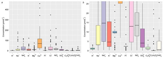
Figure 4.
Box and whisker plots for the ions identified and quantified in bulk atmospheric deposition in Lavras, from November 2017 until October 2019. Horizontal lines in the box represent the 25th, 50th, and 75th percentile values. (a) Depicts all the ionic concentrations, and (b) magnifies the species with concentrations between 0 and 25 μmolL−1.
VWM concentrations were more amenable for comparisons and were calculated for all measured ions. For the whole sampling campaign, the ions profile in VWM (molar unit) may be described in the following order: Ca2+ (45.7) > Cl− (19.1) > Na+ (16.6) > NH4+ (14.4) > Mg2+ (12.8) > NO3− (9.46) > K+ (5.48) > F− (4.00) > SO42− (3.88) > HCO2− (1.92) > C2H3O2− (1.41) > C2O42− (1.26) > H+ (0.77) µmolL−1. We identified Ca2+ as the most predominant specie accounting for 33%, which coupled with Na+ and NH4+ represents 56% of the total ionic species distribution. Similar patterns were observed in Mbita, East Africa, which also is characterized as a tropical agricultural area []. It is also valuable mentioning that Cl− was the second largest ion, contributing with 13% of the total VWM concentration.
3.4. Neutralization Factor
We calculated the NF index in order to assess the influence of alkaline species in atmospheric samples. The NFCa2+ ranged between 0.99 and 29.6 while NFMg2+ and NFNH4+ varied from 0.05 to 11.0 and from 0.01 to 7.14, respectively. Considering the mean values for the entire study period, the most important neutralizing agent of sulfuric and nitric acids was Ca2+ (NF = 6.63), followed by Mg2+ (NF = 1.54) and NH4+ (NF = 1.11), which may be considered negligible. The role of Ca2+ as a dominant neutralization cation is reasonable since the calcium presented the highest VWM for the entire period studied. On the other hand, Mg2+ contributed more than NH4+ for sample neutralization, although NH4+ presented a higher VWM concentration, suggesting that this neutralization proxy is better suited for assessing the major chemical species interactions in a rich alkaline atmosphere such as in Lavras. It should be noted that Ca2+ precursor, like calcium carbonate, was sufficient to neutralize the major atmospheric acids since most samples (n = 57–98%) showed NF higher than neutrality (NF = 1). This pattern is in agreement with the pH values found.
Similar phenomena have been observed in a number of previous studies in Brazil [,] and worldwide [,,,,]. In contrast, some studies have reported the predominance of NH4+ [,] and Mg2+ [] in the atmospheric neutralization process.
3.5. Source Identification Based on PMF Results
PMF is adopted to quantitatively analyze the emission sources of the measured ionic species. According to the S/N ratio, all species were categorized as strong, except acetate, which was classified as weak (S/N = 1.5). However, due to a large amount of data below DL (>50%), acetate and formate were classified as bad and excluded from the analysis. The PMF model was run 20 times with a seed of 76 random starting points, and a number of factors from 3 to 6 were assessed to get the optimal number of factors. The stability and reliability of the output were checked according to the following parameters: Q value, parameters of linear regression between predicted and observed concentrations, frequency distributions of the scaled residuals, G-space plots, and the physical meaning of the factor profiles. Based on the evaluation of these criteria, we identified that four factors were physically reasonable and could represent the major sources in the study region (Figure 5).
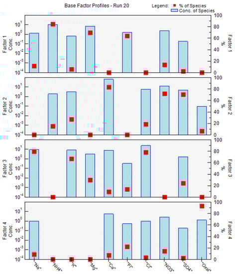
Figure 5.
Source profiles extracted by EPA PMF 5.0 model from bulk deposition samples collected in Lavras in the period between November 2017 and October 2019.
The first factor identified presented high loading values for NH4+ (85%), Mg2+ (70%), and F− (64%). The presence of F− is associated with HF gas emission, mostly from the production of steel, electrolytic aluminum, and phosphorus fertilizers [,]. Mg2+ originates naturally from marine aerosols and/or crustal particles, and its anthropogenic sources can be associated with cement industries and fertilizer production. NH4+ can be directly attributed to an input of NH3 in the atmosphere, mainly due to farming and nitrogen fertilizer production and application []. This profile corroborates with the agricultural background of the study region, where an average nitrogen and phosphor synthetic fertilizers application rate was estimated at 194 kgha−1 []. In addition, there are several agro-industrial sources inside the county air basin. Thus, this factor was categorized as fertilizer application and production.
The second factor, named atmospheric neutralization processes, was represented by Ca2+ (83%), NO3− (71%), and SO4− (70%). These species are involved in neutralizing atmospheric processes since CaCO3 is an alkaline species that neutralizes the major atmospheric acids (H2SO4 and HNO3). It should be noted that cement manufacturing and limestone mining were considered the two major sources of Ca2+ to the atmosphere in the study area. Although NO3− and SO4− have been related to the large emissions of SO2 and NOx from the combustion of fossil fuel in large urban areas [], researches carried out in agricultural areas in California, United States, associated these species with agricultural soil emissions [], which agrees with our study.
Factor 3 was loaded with Na+ (80%), K+ (67%), and Cl− (78%). These species generally originate from sea salt, crustal aerosols, and biomass burning []. In the present study, the Cl−/Na+ ratio was 1.15, which was similar to the oceanic ratio (Cl−/Na+ = 1.17), indicating marine sources intrusion. However, the K+/Na+ ratio was 0.33, which was higher than the oceanic ratio (K+/Na+ = 0.022), suggesting a large excess of K+ and, therefore, suggesting an additional source of potassium compounds in Lavras, such as biomass burning. Because of the ambiguity of sources in this factor, it was characterized as marine intrusion/biomass burning.
Factor 4 was categorized as biogenic emissions due to the high load of oxalate (93%). Organic acids in the atmosphere in large urban areas originate from motor vehicle emissions, fossil fuel combustion, and photochemical reactions. However, in rural areas, biogenic emissions, such as vegetation release and biomass burning, are more important sources of organic acids [].
4. Conclusions
We assessed bulk atmospheric deposition in a Brazilian agricultural region and observed that the pH mean was 5.99, and most deposition samples (~98%) were alkaline (pH > 5.60). In addition, the most important neutralizing agent of sulfuric and nitric acids was Ca2+ precursors (NF = 6.63). This process was corroborated by the higher abundance of Ca2+ (33%) among all ions measured. The PMF analysis resulted in four factors, which demonstrated the influence of anthropogenic and natural sources, such as fertilizer application and production, marine intrusion/biomass burning, and biogenic emissions, and revealed the importance of atmospheric neutralization processes.
The atmospheric deposition systemic analysis allowed us to monitor and evaluate the chemical transformation processes and reaction routes and to identify the polluting sources. From that, it is possible to develop emission reduction strategies, as effectively done in the previous decades for acid rain. Given this perspective, our findings are useful to understand the majority of atmospheric species sources in the Southern Minas Gerais, Brazil.
Author Contributions
Conceptualization, M.V.-F., J.N.P. and A.F.; methodology, M.V.-F., J.N.P. and A.F.; software, J.N.P.; data curation, M.V.-F. and J.N.P.; writing—original draft preparation, M.V.-F. and J.N.P.; writing—review and editing, M.V.-F., J.N.P. and A.F.; supervision, M.V.-F.; project administration, M.V.-F.; funding acquisition, M.V.-F. and A.F. All authors have read and agreed to the published version of the manuscript.
Institutional Review Board Statement
Not applicable.
Informed Consent Statement
Not applicable.
Data Availability Statement
Not applicable.
Acknowledgments
The authors thank to Coordenação de Aperfeiçoamento de Pessoal de Nível Superior (CAPES) and Fundação de Amparo à Pesquisa do Estado de Minas Gerais (Fapemig) for the Graduate and Undergraduate Scholarships. Special thanks go to “Laboratório de Processos Atmosféricos da Universidade de São Paulo (LAPAt-IAG-USP)” for the facilities and equipments used in this study.
Conflicts of Interest
The authors declare no conflict of interest.
References
- Kamani, H.; Hoseini, M. Study of trace elements in wet atmospheric precipitation in Tehran, Iran. Environ. Monit. Assess. 2014, 186, 5059–5067. [Google Scholar] [CrossRef] [PubMed]
- Araujo, T.G.; Souza, M.F.L.; De Mello, W.Z.; Da Silva, D.M.L. Bulk Atmospheric Deposition of Major Ions and Dissolved Organic Nitrogen in the Lower Course of a Tropical River Basin, Southern Bahia, Brazil. J. Braz. Chem. Soc. 2015, 26, 1692–1701. [Google Scholar] [CrossRef]
- Duan, L.; Chen, X.; Ma, X.; Zhao, B.; Larssen, T.; Wang, S.; Ye, Z. Atmospheric S and N deposition relates to increasing riverine transport of S and N in southwest China: Implications for soil acidification. Environ. Pollut. 2016, 218, 1191–1199. [Google Scholar] [CrossRef] [PubMed]
- Sun, X.; Wang, Y.; Li, H.; Yang, X.; Sun, L.; Wang, X.; Wang, T.; Wang, W. Organic acids in cloud water and rainwater at a mountain site in acid rain areas of South China. Environ. Sci. Pollut. Res. 2016, 23, 9529–9539. [Google Scholar] [CrossRef] [PubMed]
- Zhou, X.; Xu, Z.; Liu, W.; Wu, Y.; Zhao, T.; Jiang, H.; Zhang, X.; Zhang, J.; Zhou, L.; Wang, Y. Chemical composition of precipitation in Shenzhen, a coastal mega-city in South China: Influence of urbanization and anthropogenic activities on acidity and ionic composition. Sci. Total Environ. 2019, 662, 218–226. [Google Scholar] [CrossRef] [PubMed]
- Deusdará, K.R.L.; Forti, M.C.; Borma, L.S.; Menezes, R.S.C.; Lima, J.R.S.; Ometto, J.P.H.B. Rainwater chemistry and bulk atmospheric deposition in a tropical semiarid ecosystem: The Brazilian Caatinga. J. Atmos. Chem. 2017, 74, 71–85. [Google Scholar] [CrossRef]
- Szép, R.; Bodor, Z.; Miklóssy, I.; Niță, I.A.; Oprea, O.A.; Keresztesi, Á. Influence of peat fires on the rainwater chemistry in intra-mountain basins with specific atmospheric circulations (Eastern Carpathians, Romania). Sci. Total Environ. 2019, 647, 275–289. [Google Scholar] [CrossRef]
- Rastegari Mehr, M.; Keshavarzi, B.; Sorooshian, A. Influence of natural and urban emissions on rainwater chemistry at a southwestern Iran coastal site. Sci. Total Environ. 2019, 668, 1213–1221. [Google Scholar] [CrossRef]
- Moreda-Piñeiro, J.; Alonso-Rodríguez, E.; Moscoso-Pérez, C.; Blanco-Heras, G.; Turnes-Carou, I.; López-Mahía, P.; Muniategui-Lorenzo, S.; Prada-Rodríguez, D. Influence of marine, terrestrial and anthropogenic sources on ionic and metallic composition of rainwater at a suburban site (northwest coast of Spain). Atmos. Environ. 2014, 88, 30–38. [Google Scholar] [CrossRef]
- Kuzu, S.L.; Saral, A. The effect of meteorological conditions on aerosol size distribution in Istanbul. Air Qual. Atmos. Health 2017, 10, 1029–1038. [Google Scholar] [CrossRef]
- Anil, I.; Alagha, O.; Karaca, F. Effects of transport patterns on chemical composition of sequential rain samples: Trajectory clustering and principal component analysis approach. Air Qual. Atmos. Health 2017, 10, 1193–1206. [Google Scholar] [CrossRef]
- Zhang, N.; Cao, J.; He, Y.; Xiao, S. Chemical composition of rainwater at Lijiang on the Southeast Tibetan Plateau: Influences from various air mass sources. J. Atmos. Chem. 2014, 71, 157–174. [Google Scholar] [CrossRef]
- Khan, M.F.; Latif, M.T.; Saw, W.H.; Amil, N.; Nadzir, M.S.M.; Sahani, M.; Tahir, N.M.; Chung, J.X. Fine particulate matter in the tropical environment: Monsoonal effects, source apportionment, and health risk assessment. Atmos. Chem. Phys. 2016, 16, 597–617. [Google Scholar] [CrossRef] [Green Version]
- Sofowote, U.M.; Su, Y.; Dabek-Zlotorzynska, E.; Rastogi, A.K.; Brook, J.; Hopke, P.K. Sources and temporal variations of constrained PMF factors obtained from multiple-year receptor modeling of ambient PM2.5 data from five speciation sites in Ontario, Canada. Atmos. Environ. 2015, 108, 140–150. [Google Scholar] [CrossRef]
- Roy, A.; Chatterjee, A.; Tiwari, S.; Sarkar, C.; Das, S.K.; Ghosh, S.K.; Raha, S. Precipitation chemistry over urban, rural and high altitude Himalayan stations in eastern India. Atmos. Res. 2016, 181, 44–53. [Google Scholar] [CrossRef]
- Lara, L.B.L.S.; Artaxo, P.; Martinelli, L.A.; Victoria, R.L.; Camargo, P.B.; Krusche, A.; Ayers, G.P.; Ferraz, E.S.B.; Ballester, M.V. Chemical composition of rainwater and anthropogenic influences in the Piracicaba River Basin, Southeast Brazil. Atmos. Environ. 2001, 35, 4937–4945. [Google Scholar] [CrossRef]
- Almeida, G.L.M.D.; da Ferreira, E.C.M.; da Mendes, D.J.S.; Gomes, B.A.B.; do Souza, F.N.; do Silva, J.N.; Dos Santos, S.A.; Teixeira, P.B. Estudo sobre as regiões de planejamento de Minas Gerais: Sul de Minas Gerais; Fecomércio-MG: Belo Horizonte, Brazil, 2017. [Google Scholar]
- IBGE. Cidades e Estados: Lavras. Available online: https://cidades.ibge.gov.br/brasil/mg/lavras (accessed on 1 June 2019).
- EMBRAPA. Levantamento de Reconhecimento de Média Intensidade dos Solos da Zona Campos das Vertentes—MG; Embrapa Solos: Rio de Janeiro, Brazil, 2006. [Google Scholar]
- IBGE. Produção Agrícola Municipal. Available online: https://sidra.ibge.gov.br/Tabela/5457 (accessed on 3 June 2021).
- DENATRAN. Frota de Veículos. 2018. Available online: https://infraestrutura.gov.br/component/content/article/115-portal-denatran/8558-frota-de-veiculos-2018.html (accessed on 1 June 2019).
- INMET. Normais Climatológicas do Brasil. Available online: http://www.inmet.gov.br/portal/index.php?r=clima/normaisClimatologicas (accessed on 15 September 2019).
- WMO. Manual for the Gaw Precipitation Chemistry Programme: Guidelines, Data Quality Objectives and Standard Operating Procedures; GAW Precipitation Chemistry Science Advisory Group, 2004; Available online: https://library.wmo.int/doc_num.php?explnum_id=9287 (accessed on 1 June 2019).
- R Core Team. R: A Language and Environment for Statistical Computing; R Foundation for Statistical Computing: Vienna, Austria, 2019. [Google Scholar]
- Wickham, H. ggplot2: Elegant Graphics for Data Analysis; Springer: New York, NY, USA, 2016. [Google Scholar]
- Schaug, J.; Semb, A.; Hjellbrekke, A.-G.; Hanssen, J.; Pedersen, A. Data Quality and Quality Assurance Report; Norsk Institutt for Air Research (NILU): Kjeller, Norway, 1997. [Google Scholar]
- Clarke, N.; Žlindra, D.; Ulrich, E.; Mosello, R.; Derome, J.; Derome, K.; König, N.; Lövblad, G.; Draaijers, G.; Hansen, K.; et al. Manual on Methods and Criteria for Harmonized Sampling, Assessment, Monitoring and Analysis of the Effects of Air Pollution on Forests—Part XIV.; UNECE ICP Forests Programme Coordinating Centre: Eberswalde, Germany, 2016. [Google Scholar]
- Huang, D.Y.; Xu, Y.G.; Peng, P.; Zhang, H.H.; Lan, J.B. Chemical composition and seasonal variation of acid deposition in Guangzhou, South China: Comparison with precipitation in other major Chinese cities. Environ. Pollut. 2009, 157, 35–41. [Google Scholar] [CrossRef]
- Qiao, X.; Xiao, W.; Jaffe, D.; Kota, S.H.; Ying, Q.; Tang, Y. Atmospheric wet deposition of sulfur and nitrogen in Jiuzhaigou National Nature Reserve, Sichuan Province, China. Sci. Total Environ. 2015, 511, 28–36. [Google Scholar] [CrossRef]
- US-EPA. Positive Matrix Factorization Model; US EPA Research: Washington, DC, USA, 2018.
- US-EPA. EPA Positive Matrix Factorization (PMF) 5.0—Fundamentals and User Guide; Environmental Protection Agency Research: Washington, DC, USA, 2014.
- Paatero, P. Least squares formulation of robust non-negative factor analysis. Chemom. Intell. Lab. Syst. 1997, 37, 23–35. [Google Scholar] [CrossRef]
- Paatero, P.; Tapper, U. Positive matrix factorization: A non-negative factor model with optimal utilization of error estimates of data values. Environmetrics 1994, 5, 111–126. [Google Scholar] [CrossRef]
- Reff, A.; Eberly, S.I.; Bhave, P.V. Receptor modeling of ambient particulate matter data using positive matrix factorization: Review of existing methods. J. Air Waste Manag. Assoc. 2007, 57, 146–154. [Google Scholar] [CrossRef] [Green Version]
- Alves, D.D.; Backes, E.; Rocha-Uriartt, L.; Riegel, R.P.; de Quevedo, D.M.; Schmitt, J.L.; da Costa, G.M.; Osório, D.M.M. Chemical composition of rainwater in the Sinos River Basin, Southern Brazil: A source apportionment study. Environ. Sci. Pollut. Res. 2018, 25, 24150–24161. [Google Scholar] [CrossRef]
- Prathibha, P.; Kothai, P.; Saradhi, I.V.; Pandit, G.G.; Puranik, V.D. Chemical characterization of precipitation at a coastal site in Trombay, Mumbai, India. Environ. Monit. Assess. 2010, 168, 45–53. [Google Scholar] [CrossRef] [PubMed]
- Xu, H.; Bi, X.H.; Feng, Y.C.; Lin, F.M.; Jiao, L.; Hong, S.M.; Liu, W.G.; Zhang, X.-Y. Chemical composition of precipitation and its sources in Hangzhou, China. Environ. Monit. Assess. 2011, 183, 581–592. [Google Scholar] [CrossRef] [PubMed]
- Meng, Y.; Zhao, Y.; Li, R.; Li, J.; Cui, L.; Kong, L.; Fu, H. Characterization of inorganic ions in rainwater in the megacity of Shanghai: Spatiotemporal variations and source apportionment. Atmos. Res. 2019, 222, 12–24. [Google Scholar] [CrossRef]
- Akpo, A.B.; Galy-Lacaux, C.; Laouali, D.; Delon, C.; Liousse, C.; Adon, M.; Gardrat, E.; Mariscal, A.; Darakpa, C. Precipitation chemistry and wet deposition in a remote wet savanna site in West Africa: Djougou (Benin). Atmos. Environ. 2015, 115, 110–123. [Google Scholar] [CrossRef]
- Zhao, M.; Li, L.; Liu, Z.; Chen, B.; Huang, J.; Cai, J.; Deng, S. Chemical Composition and Sources of Rainwater Collected at a Semi-Rural Site in Ya’an, Southwestern China. Atmos. Clim. Sci. 2013, 03, 486–496. [Google Scholar] [CrossRef] [Green Version]
- Seinfeld, J.H.; Pandis, S.N. Atmospheric Chemistry and Physics: From Air Pollution to Climate Change, 2nd ed.; John Wiley & Sons, Inc.: Hoboken, NJ, USA, 1998; Volume 51, ISBN 9780471720171. [Google Scholar]
- Mimura, A.M.S.; Almeida, J.M.; Vaz, F.A.S.; de Oliveira, M.A.L.; Ferreira, C.C.M.; Silva, J.C.J. Chemical composition monitoring of tropical rainwater during an atypical dry year. Atmos. Res. 2016, 169, 391–399. [Google Scholar] [CrossRef]
- Bakayoko, A.; Galy-Lacaux, C.; Yoboué, V.; Hickman, J.E.; Roux, F.; Gardrat, E.; Julien, F.; Delon, C. Dominant contribution of nitrogen compounds in precipitation chemistry in the Lake Victoria catchment (East Africa). Environ. Res. Lett. 2021, 16, 045013. [Google Scholar] [CrossRef]
- Migliavacca, D.; Teixeira, E.C.; Wiegand, F.; Machado, A.C.M.; Sanchez, J. Atmospheric precipitation and chemical composition of an urban site, Guaíba hydrographic basin, Brazil. Atmos. Environ. 2005, 39, 1829–1844. [Google Scholar] [CrossRef]
- Xiao, J. Chemical composition and source identification of rainwater constituents at an urban site in Xi’an. Environ. Earth Sci. 2016, 75, 1–12. [Google Scholar] [CrossRef]
- Tositti, L.; Pieri, L.; Brattich, E.; Parmeggiani, S.; Ventura, F. Chemical characteristics of atmospheric bulk deposition in a semi-rural area of the Po Valley (Italy). J. Atmos. Chem. 2018, 75, 97–121. [Google Scholar] [CrossRef]
- Herrera, J.; Rodríguez, S.; Baéz, A.P. Chemical composition of bulk precipitation in the metropolitan area of Costa Rica, Central America. Atmos. Res. 2009, 94, 151–160. [Google Scholar] [CrossRef]
- Yatkin, S.; Adali, M.; Bayram, A. A study on the precipitation in Izmir, Turkey: Chemical composition and source apportionment by receptor models. J. Atmos. Chem. 2016, 73, 241–259. [Google Scholar] [CrossRef]
- Singh, S.P.; Khare, P.; Satsangi, G.S.; Lakhani, A.; Maharaj Kumari, K.; Srivastava, S.S. Rainwater composition at a regional representative site of a semi-arid region of India. Water. Air. Soil Pollut. 2001, 127, 93–108. [Google Scholar] [CrossRef]
- Zhang, M.; Wang, S.; Wu, F.; Yuan, X.; Zhang, Y. Chemical compositions of wet precipitation and anthropogenic influences at a developing urban site in southeastern China. Atmos. Res. 2007, 84, 311–322. [Google Scholar] [CrossRef]
- Zeng, J.; Han, G.; Wu, Q.; Tang, Y. Effects of agricultural alkaline substances on reducing the rainwater acidification: Insight from chemical compositions and calcium isotopes in a karst forests area. Agric. Ecosyst. Environ. 2020, 290, 106782. [Google Scholar] [CrossRef]
- Guo, S.H.; Gao, P.; Wu, B.; Zhang, L.Y. Fluorine emission list of China’s key industries and soil fluorine concentration estimation. J. Appl. Ecol. 2019. [Google Scholar] [CrossRef]
- Klumpp, A.; Domingos, M.; Klumpp, G. Assessment of the vegetation risk by fluoride emissions from fertiliser industries at Cubatao, Brazil. Sci. Total Environ. 1996, 192, 219–228. [Google Scholar] [CrossRef]
- IBGE. Aplicação de Fertilizantes Nitrogenados por Unidades da Federação. Available online: https://sidra.ibge.gov.br/tabela/770 (accessed on 5 June 2021).
- Almaraz, M.; Bai, E.; Wang, C.; Trousdell, J.; Conley, S.; Faloona, I.; Houlton, B.Z. Erratum: Agriculture is a major source of NOx pollution in California (Science Advances doi:10.1126/sciadv.aao3477). Sci. Adv. 2018, 4, 1–9. [Google Scholar] [CrossRef] [Green Version]
- Niu, H.; He, Y.; Zhu, G.; Xin, H.; Du, J.; Pu, T.; Lu, X.; Zhao, G. Environmental implications of the snow chemistry from Mt. Yulong, southeastern Tibetan Plateau. Quat. Int. 2013, 313–314, 168–178. [Google Scholar] [CrossRef]
- Niu, Y.; Li, X.; Pu, J.; Huang, Z. Organic acids contribute to rainwater acidity at a rural site in eastern China. Air Qual. Atmos. Health 2018, 11, 459–469. [Google Scholar] [CrossRef]
Publisher’s Note: MDPI stays neutral with regard to jurisdictional claims in published maps and institutional affiliations. |
© 2021 by the authors. Licensee MDPI, Basel, Switzerland. This article is an open access article distributed under the terms and conditions of the Creative Commons Attribution (CC BY) license (https://creativecommons.org/licenses/by/4.0/).