Hardware Implementation of an Automatic Rendering Tone Mapping Algorithm for a Wide Dynamic Range Display

Abstract

Tone mapping algorithms are used to adapt captured wide dynamic range (WDR) scenes to the limited dynamic range of available display devices. Although there are several tone mapping algorithms available, most of them require manual tuning of their rendering parameters. In addition, the high complexities of some of these algorithms make it difficult to implement efficient real-time hardware systems. In this work, a real-time hardware implementation of an exponent-based tone mapping algorithm is presented. The algorithm performs a mixture of both global and local compression on colored WDR images. An automatic parameter selector has been proposed for the tone mapping algorithm in order to achieve good tone-mapped images without manual reconfiguration of the algorithm for each WDR image. Both algorithms are described in Verilog and synthesized for a field programmable gate array (FPGA). The hardware architecture employs a combination of parallelism and system pipelining, so as to achieve a high performance in power consumption, hardware resources usage and processing speed. Results show that the hardware architecture produces images of good visual quality that can be compared to software-based tone mapping algorithms. High peak signal-to-noise ratio (PSNR) and structural similarity (SSIM) scores were obtained when the results were compared with output images obtained from software simulations using MATLAB.

1. Introduction

Dynamic range can be described as the luminance ratio between the brightest and darkest part of a scene [1,2]. Natural scenes can have a wide dynamic range (WDR) of five (or more) orders of magnitude, while commonly used conventional display devices, such as a standard LCD display have a very limited dynamic range of two orders of magnitude (eight-bit, which can represent 256 levels of radiance).

Wide dynamic range (WDR) images, which are also called high dynamic range images (HDR) in the literature, can be obtained by using a software program to combine multi-exposure images [3]. Due to recent technological improvements, modern image sensors can also capture WDR images that accurately describe real world scenery [4,5,6,7,8]. However, image details can be lost when these captured WDR images are reproduced by standard display devices that have a low dynamic range, such as a simple monitor. Consequently, the captured scene images on such a display will either appear over-exposed in the bright areas or under-exposed in the dark areas. In order to prevent the loss of image details due to differences in the dynamic range between the input WDR image and the output display device, a tone mapping algorithm is required. A tone mapping algorithm is used to compress the captured wide dynamic range scenes to the low dynamic range devices with a minimal loss in image quality. This is particularly important in applications, such as video surveillance systems, consumer imaging electronics (TVs, PCs, mobile phones and digital cameras), medical imaging and other areas where WDR images are used in obtaining more detailed information about a scene. The proper use of a tone mapping algorithm ensures that image details are preserved in both extreme illumination levels.

Several advancements have occurred in the development of tone mapping algorithms [9]. Two main categories of tone mapping algorithms exist: tone reproduction curves (TRC) [10,11,12,13,14] and tone reproduction operators (TRO) [15,16,17,18,19,20,21].

The tone reproduction curve, which is also known as the global tone mapping operator, maps all the image pixel values to a display value without taking into consideration the spatial location of the pixel in question [21]. As a result, one input pixel value results in only one output pixel value.

On the other hand, the tone reproduction operator, also called the local mapping operator, depends on the spatial location of the pixel, and varying transformations are applied to each pixel depending on its surroundings [20,22]. For this reason, one input WDR pixel value may result in different compressed output values. Most tone mapping operators perform only one type of tone mapping operation (global or local); algorithms that use both global and local operators have been introduced by Meylan et al. [21,23], Glozman et al. [22,24] and Ureña et al. [25].

There are trade-offs that occur depending on which method of tone mapping is utilized. Global tone mapping algorithms generally have lower time consumption and computational effort, in comparison to local tone mapping operators [22]. However, they can result in the loss of local contrast, due to the global compression of the dynamic range. Local tone mapping operators produce higher quality images, because they preserve the image details and local contrast. Although local tone mapping algorithms do not result in a loss of local contrast, they may introduce artifacts, such a halos, to the resulting compressed image [22,24]. In addition, most tone mapping algorithms require manual tuning of their parameters in order to produce a good quality tone-mapped image. This is because the rendering parameters greatly affect the results of the tone-mapped image. To avoid adjusting the system’s configuration for each WDR image, some developed tone mapping algorithms select a constant value for their parameters [21,26]. This makes the tone mapping operator less suitable for hardware video applications, where a variety of WDR images with different image statistics will be compressed. An ideal tone mapping system should be able to compress an assortment of WDR images while retaining local details of the image and without re-calibration of the system for each WDR image frame.

The tone mapping algorithm developed by Glozman et al. [22,24] takes advantage of the strengths of both global and local tone mapping methods, so as to achieve the goal of compressing a wide range of pixel values into a smaller range that is suitable for display devices with less heavy computational effort. The simplicity of this tone mapping operator makes it a suitable algorithm that can be used as part of a system-on-a-chip. Although it is an effective tone mapping operator, it lacks a parameter decision block, thereby requiring manual tuning of its rendering parameters for each WDR image that needs to be displayed on a low dynamic range device.

In this paper, a new parameter setting method for Glozman et al.’s operator and a hardware implementation of both the estimation block and the tone mapping operator is proposed [22,24]. The novel automatic parameter decision algorithm avoids the problem of manually setting the configuration of the tone mapping system in order to produce good quality tone-mapped images. The optimized tone mapping architecture was implemented using Verilog Hardware Description Language (HDL) and synthesized into a field programmable gate array (FPGA). The hardware architecture combines pipelining and parallel processing to achieve significant efficiency in processing time, hardware resources and power consumption.

The hardware design provides a solution for implementing the tone mapping algorithm as part of a system-on-a-chip (SOC) with WDR imaging capabilities for biomedical, mobile, automotive and security surveillance applications [1,27]. The remainder of this paper is structured as follows: Section 2 provides a review of existing tone mapping hardware architectures. Section 3 describes the tone mapping algorithm of Glozman et al. [22,24]. The details of the proposed extension of the tone mapping operator are described in Section 4. The results of the proposed optimization of the tone mapping operator are also displayed in Section 4. Section 5 explains the proposed hardware architecture in detail. In Section 6, the hardware cost and synthesis details of the full tone mapping system are given. Comparisons with other published hardware designs in terms of image quality, processing speed and hardware cost are also presented in Section 6. In addition, simulation results of the automated hardware implementation using various WDR images obtained from the Debevec library and other sources are shown in Section 6. Finally, conclusions are presented in Section 7.

2. Related Works on Tone Mapping Systems

2.1. Tone Mapping Implementations: Hardware vs. Software

Tone mapping algorithms can be executed on either hardware or software systems or on an incorporation of both. A high number of successful tone mapping algorithms have been implemented on software platforms [12,17,18,19,20,21,26,28,29,30,31,32]. For software implementations, the tone mapping operator is applied on the stored image using a programmed application on a PC workstation. Different tone mapping algorithms with varying complexities can be easily developed in software. Although this is advantageous, because modifications to the software code can be made quickly, complications may arise when trying to implement a tone mapping system with high processing speed for WDR video technology applications. Software systems can achieve real-time implementation for global tone mapping systems. Although global tone mapping algorithms have a shorter computational time, they may result in a loss of local contrast in WDR images. In contrast, complications may arise when implementing local tone mapping algorithms, due to computational complexity and the time required for these algorithms to process one image frame [29]. In addition, software implementation of a tone mapping system will not satisfy our goal of having the architecture embedded as part of a system on chip.

There are a lot of hardware-based platforms, such as graphic processing units (GPUs), field programmable gate arrays (FPGAs), application-specific integrated circuits (ASICs) etc., that can be used to achieve real-time operation for both global and local tone mapping systems. Hardware-based implementations have an added advantage over software developed systems in terms of the ability of embedding the tone mapping system as part of a portable camera device for applications, such as consumer imaging electronics (TVs, PCs, mobile phones and digital cameras), medical imaging, video surveillance systems etc. Captured images can be processed pixel-by-pixel within the WDR image sensor silicon without the need of external memory buffers, thereby reducing the amount of power consumed and the area occupied by the tone mapping operators.

The tone mapping hardware system discussed in this paper was developed for a low cost FPGA device as a proof of concept. It can be further implemented in ASIC as part of a system-on-a-chip with a WDR image sensor for high volume production. In addition, a comparison with other FPGA-based tone mapping systems available in terms of hardware resources, processing speed and power consumption is presented. It should be noted that no hardware-based design of an exponent-based tone mapping operator [22,24] has been implemented and no automatic parameter decision algorithm has been proposed for it, either. This is the main thrust of this work.

2.2. Related Research on Hardware-Based Tone Mapping

There have been a few hardware-based implementations of tone mapping operators. An FPGA-based architecture by Hassan et al. [33] implements a modification of the local tone mapping operator by Reinhard et al. [18]. Modifications were made to the original local tone mapping operator in order to reduce the hardware complexity of the algorithm. It was implemented on an Altera^® Stratix II FPGA operating at 60 frames per second for a 1024 × 768 pixel image. A patent was filed for the above hardware implementation with an extension of the algorithm for colored WDR images [34].

Chiu et al. [35] presented an application-specific integrated circuit (ASIC) implementation of both the global tone mapping operator by Reinhard et al. [18] and gradient compression by Fattal et al. [26] using an ARM-SOC platform. The tone mapping processor can compress a 1024 × 768 image at 60 frames per second (fps) with an operating frequency of 100 MHz. It also occupies a core area of 8.1 mm${}^2$ under TSMC 0.13 μm technology.

Vytla et al. [36] implemented another real-time hardware tone mapping algorithm based on the gradient domain dynamic range compression by Fattal et al. [26]. A modified Poisson solver is utilized in order to reduce the hardware complexity of the original Poisson equation. A processing speed of 100 fps at a maximum operating frequency of 114.18 MHz was achieved for a one megapixel frame using the Stratix II FPGA.

A new global and local tone mapping algorithm by Ureña et al. [25] was designed and implemented on a GPU NVIDIA ION2 and Xilinx^® Spartan III FPGA for VGA resolution WDR images (640 × 480). The tone mapping operator can adapt VGA images at 30 fps and 60 fps for the GPU and FPGA device, respectively. In addition, a power consumption of 900 mV was achieved for an FPGA-based system with the same image resolution [37].

Kiser et al. [38] recently implemented on a Xilinx^® Spartan VI FPGA the global tone mapping algorithm by Reinhard et al. [18], as well as its automatic parameter estimation method for tuning one of the rendering parameters [39].

In general, the hardware-based designs presented so far can compress WDR images in real-time using the different tone mapping algorithms implemented. In this paper, however, we focused on designing an efficient hardware tone mapping system by optimizing the tone mapping algorithm of Glozman et al. [22,24] and implementing the improved tone mapping design in an FPGA device that will be used along with a WDR CMOS imager for real-time image compression. The motivation here is to later integrate the tone mapping system within a single silicon as part of a system-on-a-chip with WDR image capture capabilities. Our tone mapping system requires fewer hardware resources, lower power consumption and has higher processing speed when compared to other’s work in the past. This is achieved by using a combination of parallel processing along with pipelining to achieve significant efficiency in processing time, hardware resources and power consumption.

3. Tone Mapping Algorithm for Current Work

The tone mapping algorithm used in this work was originally designed by Glozman et al. [22,24]. It performs a mixture of both global and local compression on colored WDR images. The aim of Glozman et al. [22,24] was to produce a tone mapping algorithm that does not require heavy computational effort and can be implemented as part of a system on a chip with a WDR image sensor. In order to achieve this, they obtained inspiration from the approach proposed by Meylan et al. 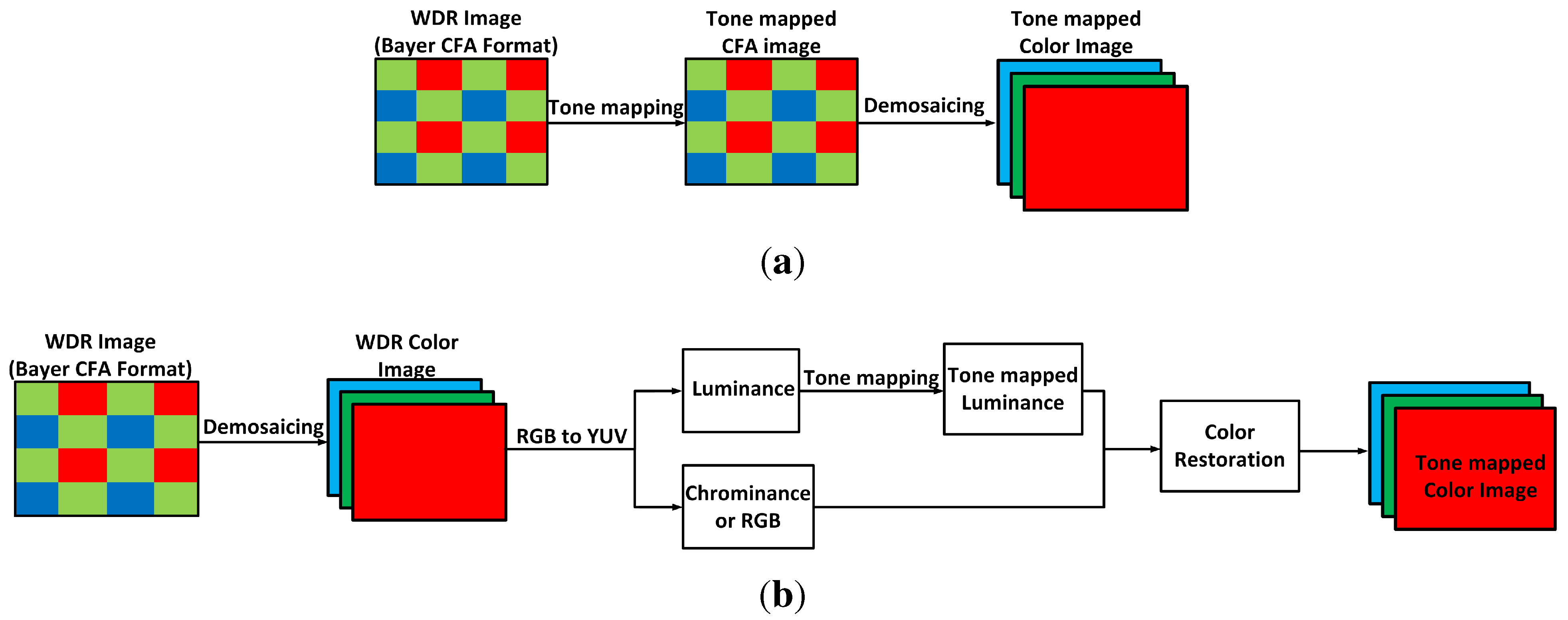[21] that involves directly implementing the tone mapping operator on the Bayer color filter array (CFA). This is different from other traditional tone mapping systems that apply the tone mapping algorithm after demosaicing the Bayer CFA image. A visual comparison of the two different color image processing workflow is shown in Figure 1. In traditional color image processing workflow, the image is first converted to YUV or HSV color space (luminance and chrominance), and the tone mapping algorithm is then applied on the luminance band of the WDR image [18,25,26]. The chrominance layer or the three image color components (R, G, B) are stored for later restoration of the color image [26]. This is not ideal for a tone mapping operator that will be implemented solely on a system-on-a-chip because additional memory is needed to store the full chrominance layer or the RGB format of the image. In contrast, no extra memory is required to store the chrominance layer of the colored image being processed in Glozman et al.’s tone mapping approach, since it uses the monochrome Bayer image formed at the image sensor [22,24]. Furthermore, no additional computation is required for calculating the luminance layer of the colored image, thereby reducing the overall computational complexity of our algorithm.

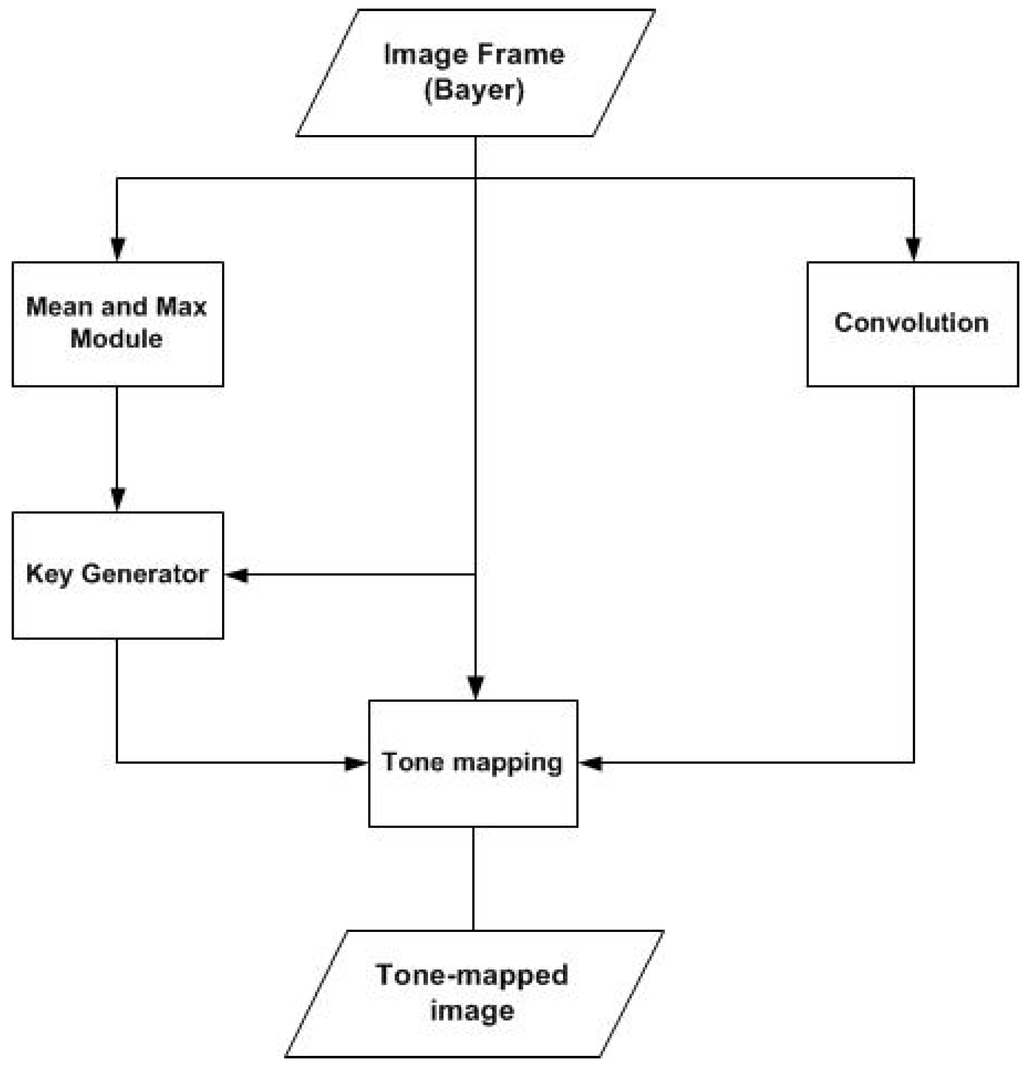
Figure 1. (a) Workflow approach proposed by Meylan et al. [21] and implemented in Glozman et al.’s tone mapping algorithm [22,24]; (b) Detailed block description of a traditional color image processing workflow for tone mapping wide dynamic range (WDR) images.

Figure 1. (a) Workflow approach proposed by Meylan et al. [21] and implemented in Glozman et al.’s tone mapping algorithm [22,24]; (b) Detailed block description of a traditional color image processing workflow for tone mapping wide dynamic range (WDR) images.

Glozman et al.’s tone mapping model takes inspiration from an inverse exponential function, which is one of the simplest nonlinear mappings used in adapting a WDR image to the limited dynamic range of display devices [22,24,29]. The inverse exponential function is defined as follows [29]:

$$Y\left(p\right)=1-{exp}^{-\frac{X\left(p\right)}{X_o\left(p\right)}}$$

(1)

where p is a pixel in the CFA image; $X\left(p\right)$ represents the input light intensity of pixel p; $Y\left(p\right)$ is the pixel’s tone-mapped signal and $X_o\left(p\right)$ is the adaptation factor. $X_o\left(p\right)$ is a constant for every pixel, and it is given by the mean of the entire CFA image. In Glozman et al.’s tone mapping algorithm [22,24], the adaptation factor, $X_o\left(p\right)$, varies for each WDR pixel, and it is defined by:

$$X_o\left(p\right)=k·X_{DC}+(X\ast F_w)\left(p\right)$$

(2)

where p is a pixel in the image; $X_o\left(p\right)$ is the adaptation factor at pixel p; $X_{DC}$ is the mean value of all the CFA image pixel intensities; * represents the convolution operation and $F_w$ is a two-dimensional Gaussian filter. The output of the convolution is used in providing the local adaptation value for each CFA pixel, since that output depends on the neighborhood of the CFA pixel. The factor, k, is a coefficient, which is used in adjusting the amount of global component in the resulting tone-mapped image. Its value ranges from zero to one, depending on the overall tone of the image.

The new adaptation factor for the proposed tone mapping algorithm Equation (2) ensures that different tonal curves are applied to each pixel depending on the spatial location of the image pixel. This is different from the original inverse exponential tone mapping function that applies the same tonal curve to all the pixels in the WDR image.

A scaling coefficient is also added to Equation (1), so as to ensure that all the tone mapping curves will start at the origin and meet at the maximum luminance intensity of the display device. The full tone mapping function is defined as follows:

$$Y\left(p\right)=\frac{\alpha }{1-{exp}^{-\frac{X_{max}}{X_o\left(p\right)}}}·\left(1-ex{p}^{-\frac{X\left(p\right)}{X_o\left(p\right)}}\right)$$

(3)

where Xmax is the maximum input light intensity of the WDR image; X, and α is the maximum pixel intensity of the display device. For standard display devices, such as a computer monitor, $\alpha =255$ (eight bits).

4. Proposed Automatic Parameter Estimation for the Exponent-Based Tone Mapping Operator

Glozman et al.’s operator is a tone mapping algorithm that compresses a WDR image based on its global and local characteristics [22,24]. It consists of global and local components that are used in the adaptation of a WDR image as given in Equations (2) and (3). The global component in adaptation factor $X_o\left(p\right)$ is comprised of factor k and the average of the image $X_{DC}$. The factor, k, is used in modulating the amount of global tonal correction $X_{DC}$ that is done to the WDR image. It can be adjusted between zero and one, depending on the image key. The image key is a subjective quantification of the amount of light in a scene [18]. Low key images are images that have a mean intensity that is lower than average, while high key images have a mean intensity that is higher than average [40]. Analysis shows that low key WDR images require factor k values closer to zero, while factor k values closer to one are required for high key WDR images. This is because the lower the k value, the higher the overall image mean. On the other hand, the higher the k value, the greater the compression of higher pixel values, resulting in a less exposed tone-mapped image. 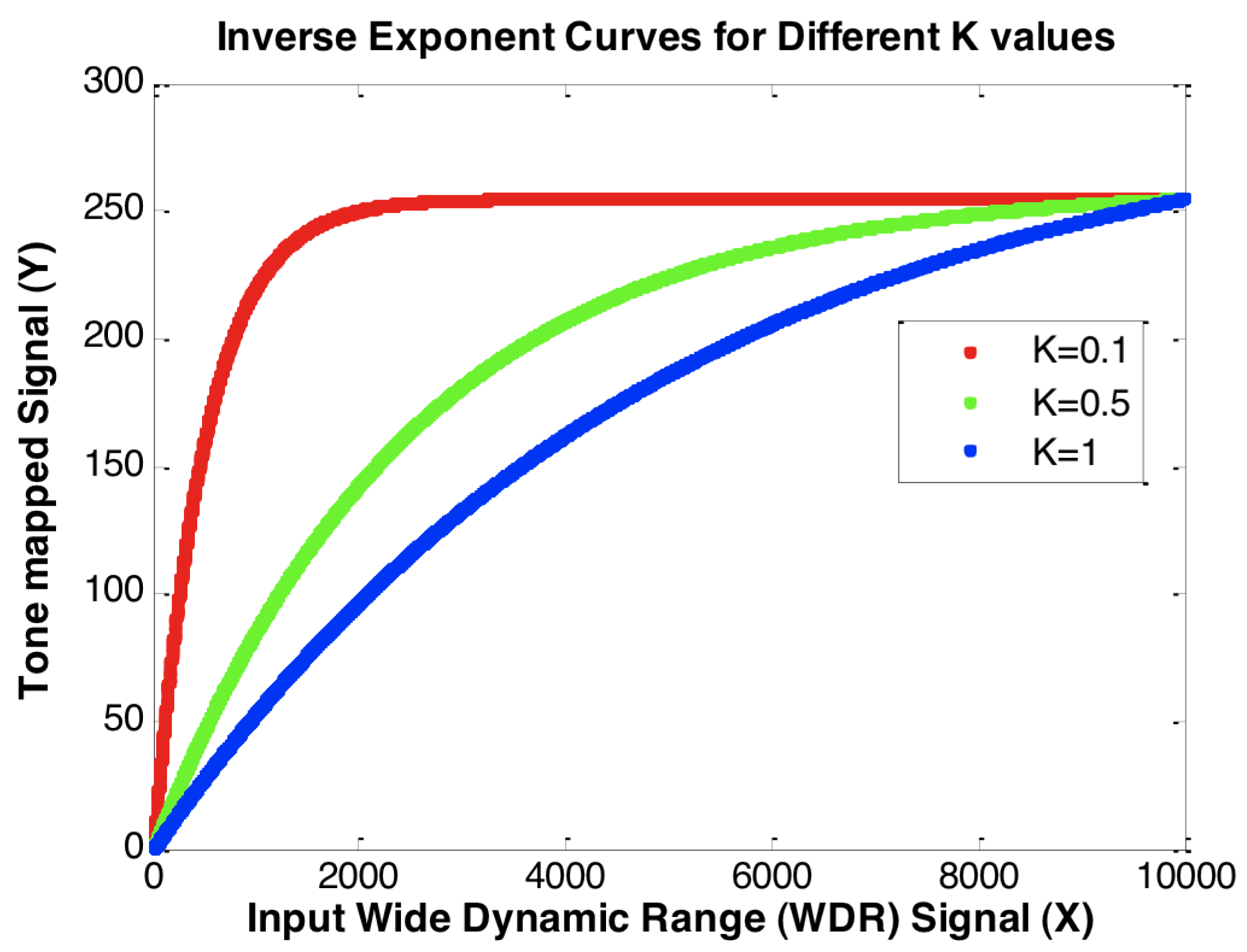To visually demonstrate the sole effect of the factor k on the tonal curve applied to the input WDR signal X, the local adaptation, $(X\ast F_w)\left(p\right)$, is kept constant, or it is assumed that there are no variations in the intensity of the surrounding pixels for each pixel in X, while the parameter k is used for performing tone mapping varies from $0.1$ to one (Figure 2).

Figure 2. Inverse exponent curves for different k values [assuming $(X\ast F_w)\left(p\right)$ is constant for the given WDR input X].

Figure 2. Inverse exponent curves for different k values [assuming $(X\ast F_w)\left(p\right)$ is constant for the given WDR input X].

As shown in Figure 2, as the factor k decreases, more of the input WDR signal X is compressed to the higher ranges of the low dynamic range device (in this case, closer to 255). This results in an increase in the overall brightness of the image as factor k decreases. Thus, the rendering parameter k needs to be adjusted automatically in order to make the tone mapping system more compact for a system-on-a-chip application.

4.1. Developing the Automatic Parameter Estimation Algorithm

The aim was to design a simple hardware-friendly automatic parameter selector for estimating factor k, so that natural looking tone-mapped images can be produced using Glozman et al.’s tone mapping algorithm [22,24]. The proposed algorithm has to be hardware-friendly, so that it can be implemented as part of the tone mapping system without dramatically increasing the power consumption and hardware resources utilized. To derive this k-equation, a mathematical model based on the properties of the image needs to be obtained experimentally. The initial hypothesis is that there exists a one-dimensional interpolation function for computing the k value. Based on this hypothesis, the k-equation can be described as shown in Equation (4):

$$k=f\left(x\right)$$

(4)

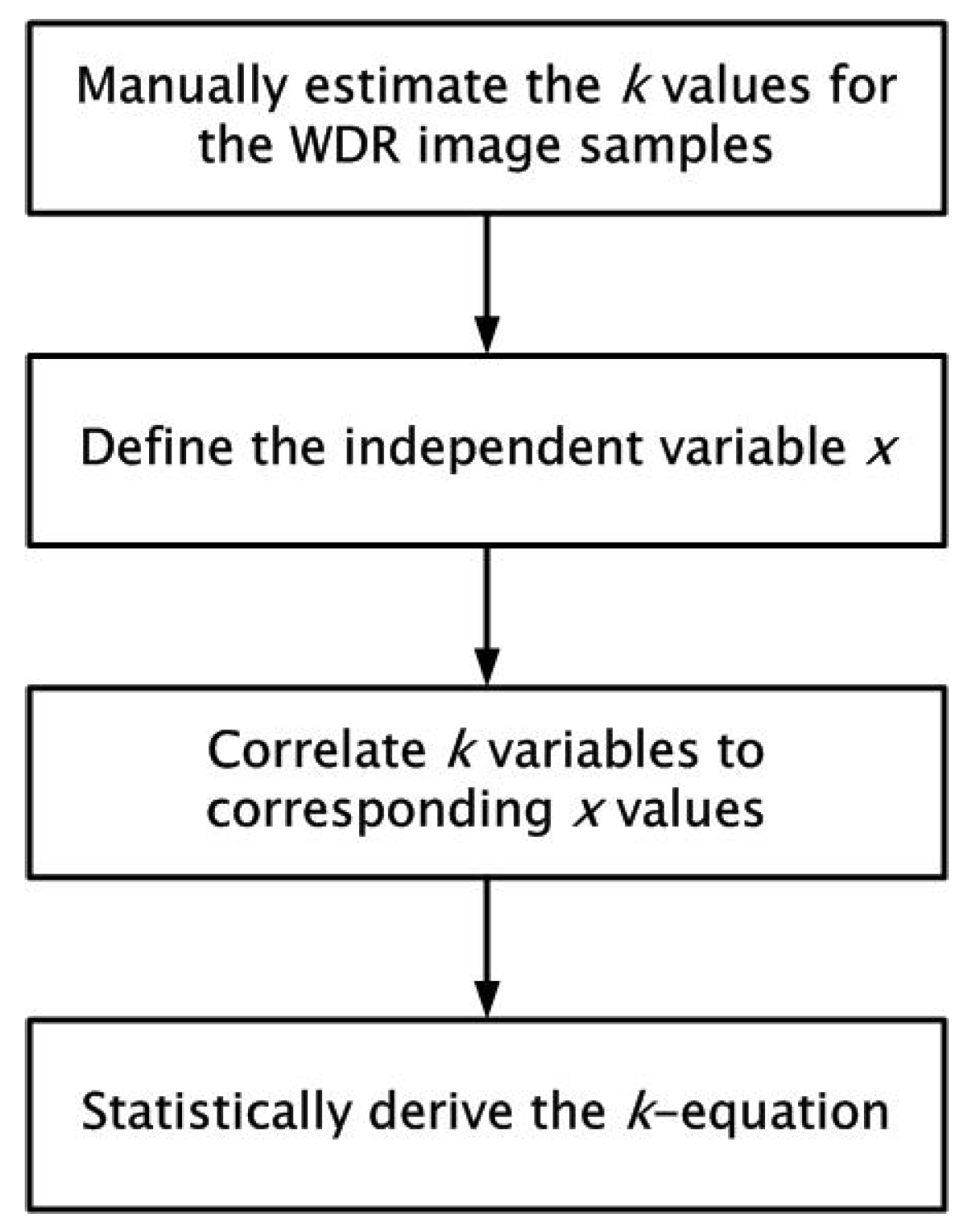
where k is the dependent variable that is applied with the adaptation equation [Equation (2)], which varies from zero to one, and x is an independent property of the WDR image. Since the function needs to be derived experimentally, the next step was to obtain the data samples used in modelling the algorithm. An outline of the steps taken in modeling the automatic estimation algorithm is shown in Figure 3. First, 200 WDR images were tone-mapped in order to obtain good quality display outputs, and their respective k values were stored. Then, the same WDR images were analyzed, and various independent variables were proposed and computed for each WDR image. Finally, the k values, as well as the different proposed independent variables were used in determining if a one-dimensional relationship exists between the selected k values and their corresponding independent variables. This is so that an equation can be derived for estimating the value k for producing good quality tone-mapped images.

Figure 3. Outline of the steps taken in deriving the mathematical model for estimating the k value needed for the tone mapping operation.

Figure 3. Outline of the steps taken in deriving the mathematical model for estimating the k value needed for the tone mapping operation.

4.1.1. Manually Estimating the Values of k

In order to develop an automatic parameter estimation algorithm, a way of manually determining which values of k produced tone-mapped images that can be deemed natural looking had to be found. Previous studies on perceived naturalness and image quality have shown that the observed naturalness of an image correlates strongly to the characteristics of the image, primarily brightness, contrast and image details [41,42,43]. As previously highlighted, the factor k is a major parameter in the tone mapping algorithm, and its value may vary for different WDR images. Analysis performed showed that the value of k predominately affects the brightness level of the tone-mapped image, but also influences the contrast of the image, due to the increase or decrease of the image brightness, as shown in Figure 2. The amount of contrast and preserved image details is primarily determined by the local adaptation component of the tone mapping algorithm [22,24]. Since the goal here was to derive a simple one-dimensional interpolation function for computing factor k for the purpose of easy hardware implementation, our focus was mainly on selecting what level of brightness was good enough for a tone-mapped image. This resulted in the issue of how to quantitatively determine how bright a tone-mapped image should be in order for it to be categorized as being of good quality.

The statistical method by Jobson et al. [41] was used in estimating what the illumination range should be in order for an image to be perceived as being a visually pleasant image. In Jobson et al.’s work, they developed an approach of relating a visually pleasant image to a visually optimal region in terms of its image statistics, i.e., image luminance and contrast. The overall image luminance is measured by calculating the mean of the image’s luminance, μ, while the contrast σ is measured by calculating the global mean of the regional standard deviations. 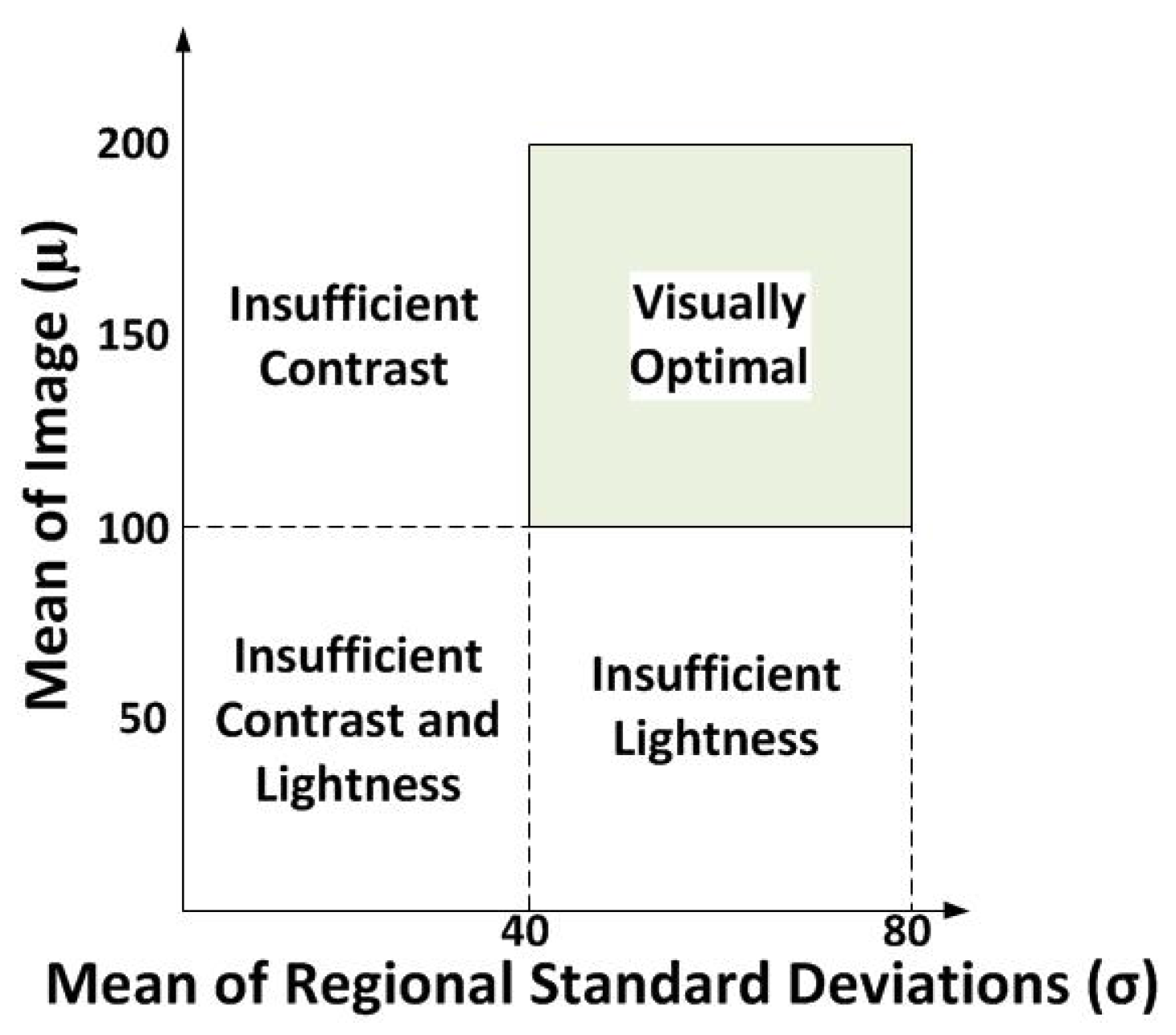To obtain the regional standard deviations, non-overlapping area blocks of 50 × 50 pixel size were used to calculate the standard deviation of a pixel region in their experiment [41]. The size of the pixel regions for computing the standard deviation can be modified. Based on the results from their experiment, they concluded that a visually optimal image was found to have high image contrast, which lies within 40–80, while its image luminance is within 100–200 for an eight-bit image or, more specifically, around the midpoint of the images dynamic range [41]. This is to ensure that the image has a well-stretched histogram. Figure 4 shows the diagram of the visually optimal region for an image in terms of its image luminance and contrast [41].

Figure 4. The four image quality regions partitioned by image luminance and image contrast [41].

Figure 4. The four image quality regions partitioned by image luminance and image contrast [41].

Using Jobson et al.’s theory, an experiment involving 200 WDR images was performed in order to obtain k values for the 200 tone-mapped images. In addition, the tone mapping image quality assessment tool by Yeganeh et al. [42] was used to ensure that the selected k values and the corresponding tone-mapped images were within the highest image quality scores attainable by the tone mapping algorithm. This objective assessment algorithm produces three image quality scores that are used in evaluating the image quality of a tone mapped image: the structural fidelity score (S), the image naturalness (N) score and the tone mapping quality index (TMQI). The structural fidelity score is based on the structural similarity (SSIM) index, and it calculates the structural similarity between the tone-mapped image and the original WDR image. The naturalness score is based on a statistical model that perceives that the naturalness of an image correlates with the image’s brightness and contrast. The overall image quality measure, which the authors call the tone mapping quality index (TMQI), is computed as a non-linear combination of both the structural similarity score (S) and the naturalness score (N). The three scores generally range from zero to one, where one is the highest in terms of image quality. 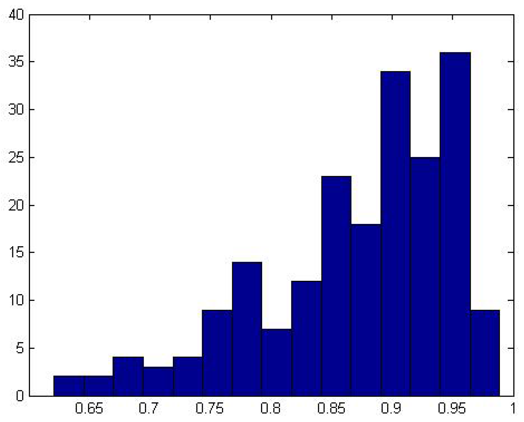Figure 5 shows the histogram of the TMQI scores for the 200 WDR images. Since the tone mapping algorithm developed by Glozman et al. [22,24] is applied on a CFA image instead of the luminance layer, the calculation of the overall image mean and contrast was based on the mean of the CFA image, as well as the mean of the regional standard deviations, respectively.

Figure 5. Histogram of the tone mapping quality index (TMQI) scores of the 200 tone-mapped images.

Figure 5. Histogram of the tone mapping quality index (TMQI) scores of the 200 tone-mapped images.

4.1.2. Determining the Independent Variable x

After performing the previous experiment where the “optimal” k values for 200 WDR images were obtained, the next step was to find a variable that correlates with these k values, so that the value of k can be predetermined before the actual tone mapping process.

An approach based on deriving an independent variable from an initially compressed WDR image was proposed. This is because WDR images can be seen as belonging to different classes, depending on the image’s dynamic range, and this may affect the interpretation of the image’s statistics. For example, a 10-bit WDR image (for which the intensity ranges from zero to $2^{10}-1$), with a mean of 32, may be different from a 16-bit WDR image (zero to $2^{16}-1$) with the same mean, due to the large difference in dynamic range. Since the goal here is to design a parameter estimation algorithm for Glozman et al.’s tone mapping operator that can be robust enough to estimate the k values for a large variety of WDR images (anything greater than eight bits), all the different WDR images need to be normalized to the same dynamic scale, so as to remove the effect of the different dynamic ranges.

The initial image compression stage is done using a simplified version of Glozman et al.’s tone mapping operation [Equation (3)]. Here, the scaling factor is removed, and the tone mapping algorithm is simplified to this:

$$Y\left(p\right)=\alpha ·\left(1-{exp}^{-\frac{X\left(p\right)}{X_o\left(p\right)}}\right)$$

(5)

$$X_o\left(p\right)=k·X_{DC}+(X\ast F_w)\left(p\right)$$

(6)

where $Y\left(p\right)$ is the tone-mapped image used for estimation; α is the maximum pixel intensity of the display device and $X_o\left(p\right)$ is the adaptation factor, which is the same as that in Glozman et al.’s operator [Equation (2)]. For standard display devices, such as a computer monitor, $\alpha =255$ (eight bits). For the adaptation function [Equation (6)], k was kept constant at 0.5, while the sigma and kernel size for the Gaussian filter was set to $\sigma =3$ and $9\times 9$, respectively.

Using the compressed image, four potential independent variables were investigated: minimum, maximum, mean and image contrast. These variables along with the WDR image’s k values are compared in order to determine if there exists a correlation. The variables that have a one-dimensional relationship with the k value applied in the actual tone mapping operation are then used in statistically-deriving a k-equation. It should be noted that the same WDR images used in obtaining the 200 k values in the previous experiment were used for deriving the four potential variables.

4.1.3. Correlation between k and the Proposed Independent Variables

In order to derive an algorithm for estimating the values of k needed for tone mapping WDR images, the computed minimum, maximum, contrast and mean values of the 200 compressed images were analyzed. Results showed that there is a correlation between the mean ($y_m$) of the initial compressed image and the k value used in the actual tone mapping operation. As shown in Figure 6, the trend of the values of k selected for the varying images correlate with the description of the rendering parameter k. As expected, low k values are required for images with a lower-than-average mean intensity, while high k values are needed for WDR images with higher-than-average mean intensity. Thus, dark WDR images that appear as low key images require low k values for the actual tone mapping process, which, in fact, improves the brightness of the image, while the reverse occurs for extremely bright WDR images.

The results also show that there is no strong one-dimensional relationship between the tone-mapped image’s contrast and the selected k value. Thus, in order to simplify the automatic parameter estimation model, the initial tone-mapped image contrast was not included in the derivation of the k-equation. Similar observations were found in the analysis of the minimum and maximum results. Hence, only the mean of the initially-compressed images was used in derivation of the estimation algorithm, and it will be used as the independent variable of the function [Equation (4)].

To obtain a relatively simple k-equation that can be implemented in hardware, the graph of k was divided into three regions (A, B, C). Region A represents extremely low independent variable $y_m$ values; and the value of k in this region is kept constant [Equation (7)]. In Region C, the k value is also kept constant, and the region represents extremely high independent variable $y_m$ values. Finally, Region B represents the region between the low and high range for the independent variable $y_m$. Using MATLAB^®’s curve fitting tool, a k-Equation (7) was obtained for Region B, which should be easy to implement in hardware.

$$k=\left\{\begin{array}{cc}0.035,\hfill & \text{if}{y}_m\le 27.16\hfill \\ 0.01439\times 2^{0.04728·y_m},\hfill & \text{if}27.16<y_m<108.25\hfill \\ 0.5,\hfill & \text{otherwise}\hfill \end{array}\right.$$

(7)

Figure 6. The graph of the mean of the initially-compressed image against the selected k for the 200 WDR images used in the experiment.

Figure 6. The graph of the mean of the initially-compressed image against the selected k for the 200 WDR images used in the experiment.

To evaluate the fit of the curve attained in Region B, the goodness of fit for the curve is computed. There are three criteria used in the analysis of these curves: the sum of squares due to error (SSE), R-squared and the root mean squared error (RMSE). The SSE is used to measure the total variation of the model’s predicted values from the observed values [44]. A better fit is indicated by a score closer to zero. R-squared is used to measure how well the curve fit explains the variations in the experiment data [44,45]. It can range from zero to one, where a better fit is indicated by a score closer to one. RMSE is used to measure the difference between the model’s predicted values and the experimentally-derived values [45]. A better fit is indicated by an RMSE value closer to zero. Results show that good SSE, RMSE and R-squared were attained for the fit. The SSE, RMSE and R-squared scores for the curve obtained in Region B were found to be 0.23300, 0.93160 and 0.03549, respectively.

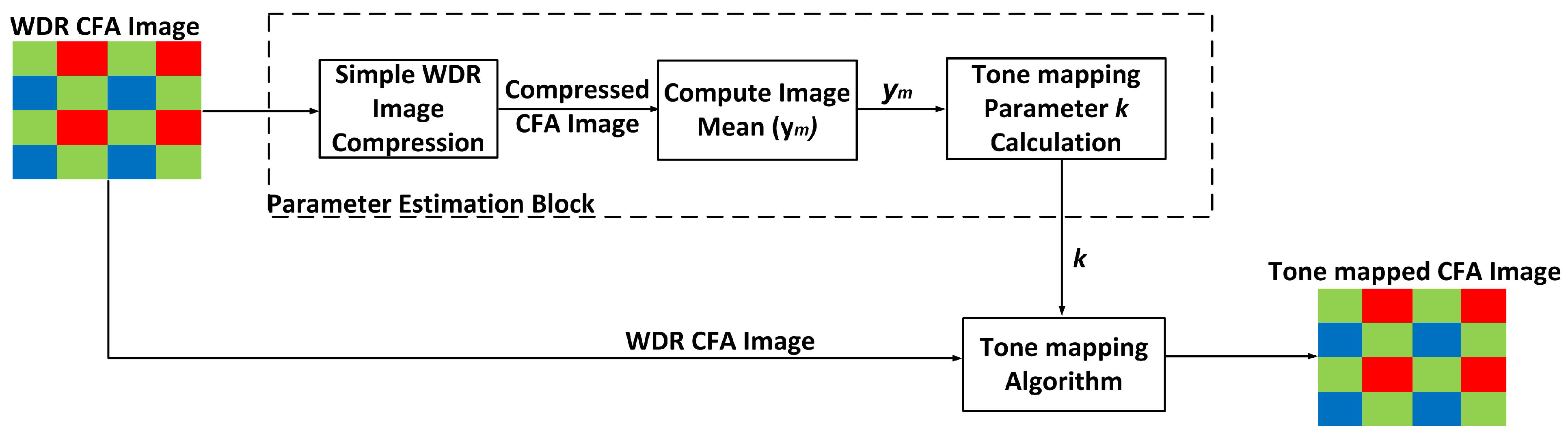
Using the derived equation from the estimation model, a pathway for performing an automatic tone mapping on a WDR image was designed. This automatic pathway is shown in Figure 7. First, an estimation of the image statistics is performed by computing the mean of the initial compressed WDR image $y_m$ using the simpler tone mapping algorithm mentioned above. Next, a k value is calculated using an estimation algorithm. This k value is then used for the actual tone mapping process using Glozman et al.’s operator [22,24].

Figure 7. Block diagram of the pathway used in performing automatic image compression of WDR images.

Figure 7. Block diagram of the pathway used in performing automatic image compression of WDR images.

4.2. Assessment of the Proposed Extension of Glozman et al.’s Tone Mapping Operator

To demonstrate that the model [Equation (7)] produces satisfactory results for a variety of WDR images, the models were tested on images that were not used in deriving the equations. The objective assessment tool index by Yeganeh et al. [42] was used in selecting the k values for the manual implementation of Glozman et al.’s tone mapping operator. The k values that were used to produce images with the highest TMQI score attainable by the tone mapping algorithm were selected. Figure 8 and Figure 9 show examples of the results from the automatic and manual-tuned tone mapping systems. Results show that the automatic rendering parameter model works well in estimating the parameter k. The image results produced using the automatic rendering parameter algorithm are similar to those obtained from manually tuning the tone mapping operator to conclude that the automatic rendering parameter model is suitable for compressing a variety of WDR images.

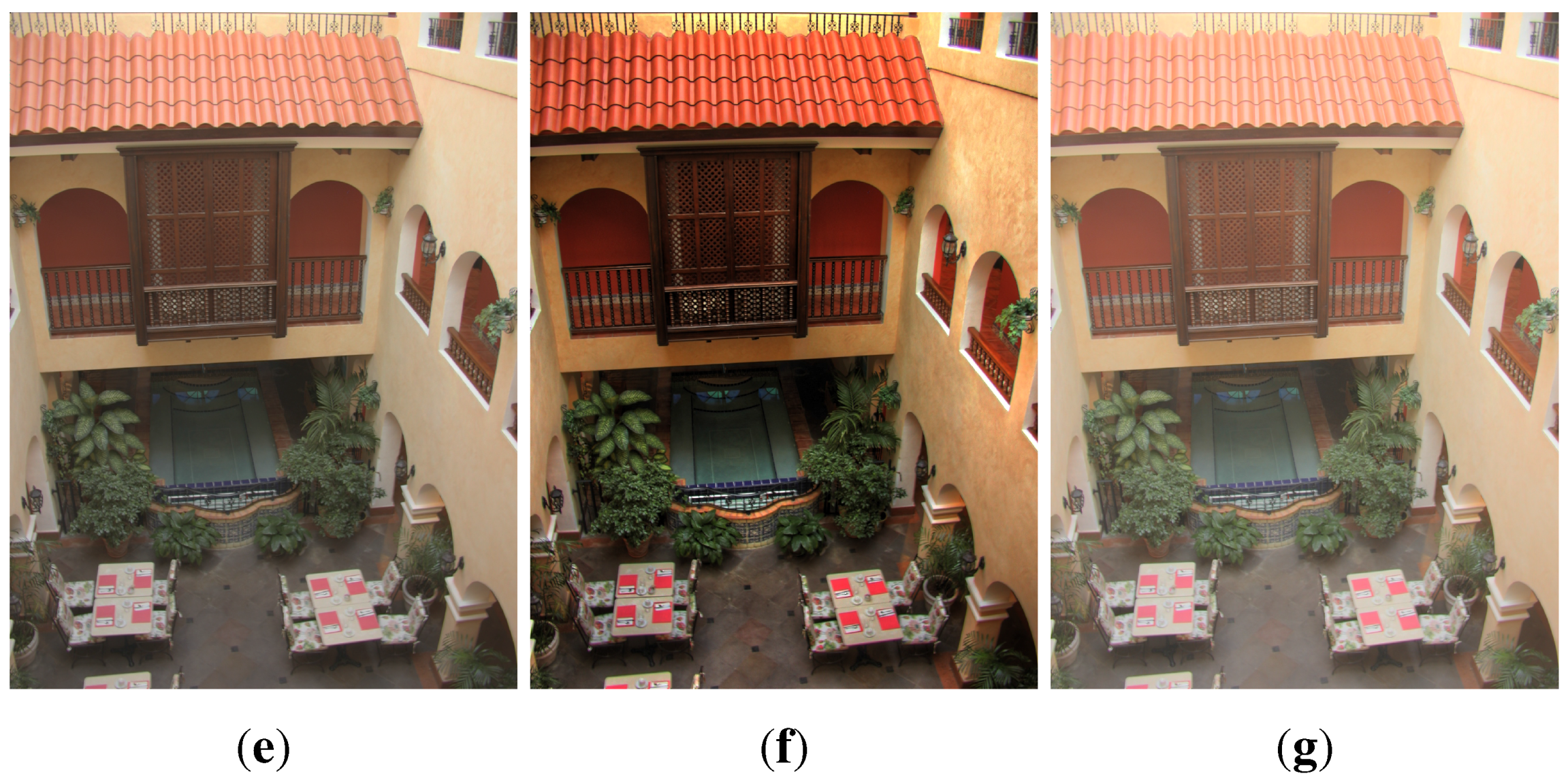
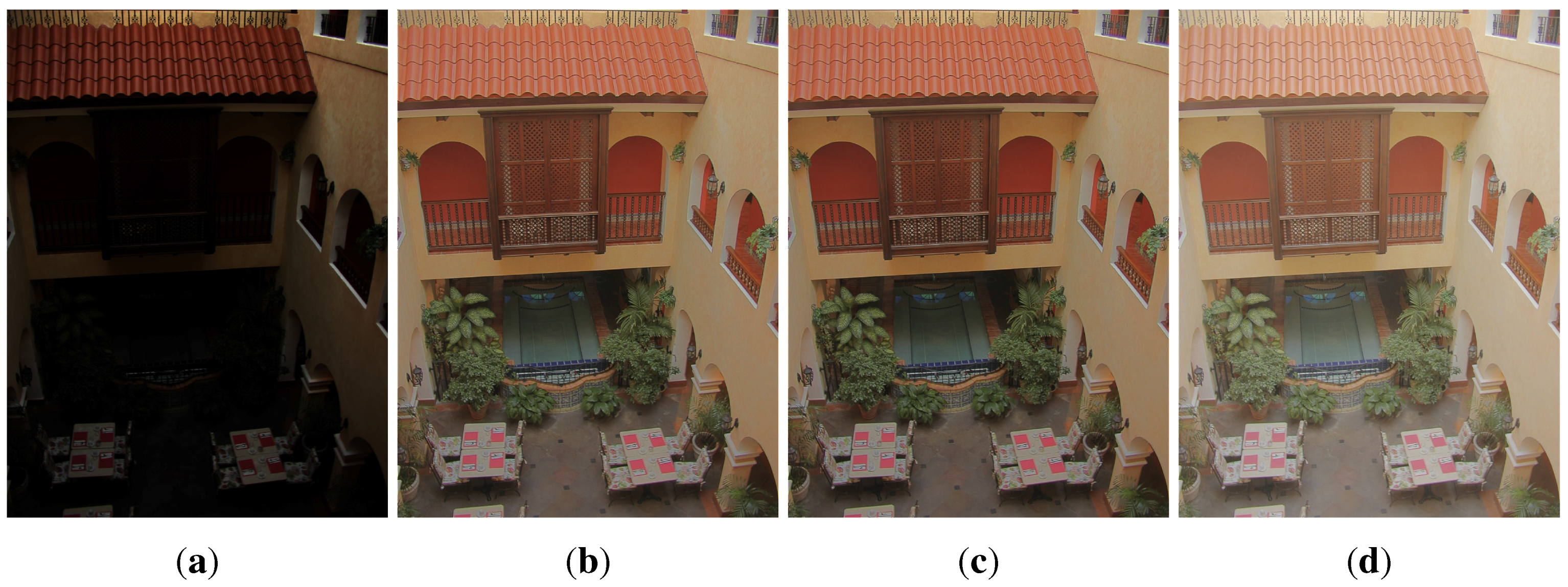
Figure 8. Tone mapped multi-fused image obtained using (a) Linear mapping; (b) Manually tuned Glozman et al.’s operator (k = 0.270) [22,24]; (c) The proposed automatic tone mapping algorithm (k = 0.278) [22,24]; (d) Meylan et al.’s operator [21]; (e) Reinhard et al.’s operator [18]; (f) The gradient-based tone mapping operator by Fattal et al. [26]; and (g) Drago et al.’s operator [12].

Figure 8. Tone mapped multi-fused image obtained using (a) Linear mapping; (b) Manually tuned Glozman et al.’s operator (k = 0.270) [22,24]; (c) The proposed automatic tone mapping algorithm (k = 0.278) [22,24]; (d) Meylan et al.’s operator [21]; (e) Reinhard et al.’s operator [18]; (f) The gradient-based tone mapping operator by Fattal et al. [26]; and (g) Drago et al.’s operator [12].

Figure 9. Tone mapped multi-fused image obtained using (a) linear mapping; (b) manually tuned Glozman et al.’s operator (k = 0.165) [22,24]; (c) the proposed automatic tone mapping algorithm (k = 0.177) [22,24]; (d) Meylan et al.’s operator [21]; (e) Reinhard et al.’s operator [18]; (f) the gradient-based tone mapping operator by Fattal et al. [26]; and (g) Drago et al.’s operator [12].

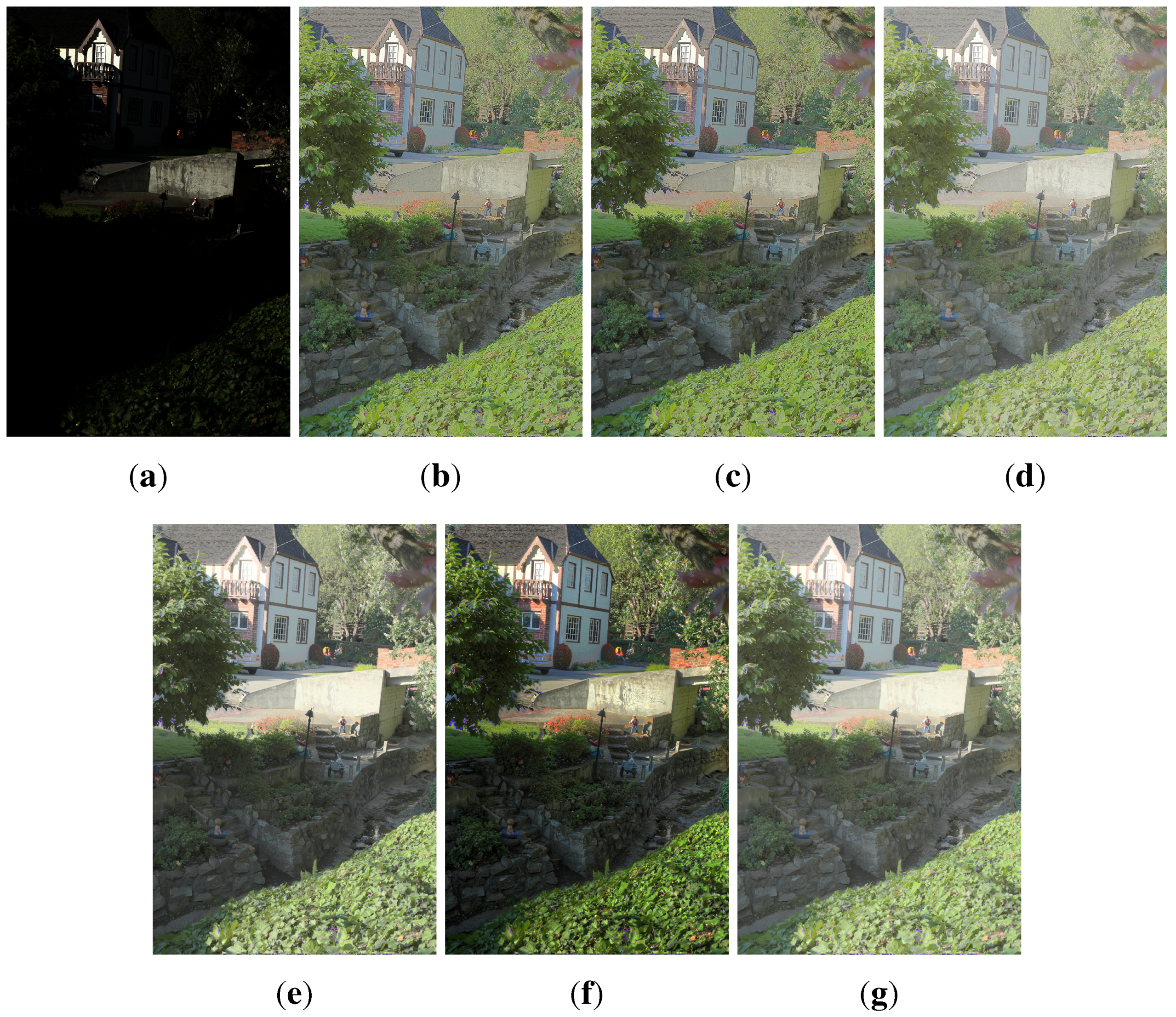
Figure 9. Tone mapped multi-fused image obtained using (a) linear mapping; (b) manually tuned Glozman et al.’s operator (k = 0.165) [22,24]; (c) the proposed automatic tone mapping algorithm (k = 0.177) [22,24]; (d) Meylan et al.’s operator [21]; (e) Reinhard et al.’s operator [18]; (f) the gradient-based tone mapping operator by Fattal et al. [26]; and (g) Drago et al.’s operator [12].

Furthermore, a quantitative assessment was performed using the objective test developed by Yeganeh et al. [42], so as to compare the output images (manually tuned and automatically rendered) with other tone mapping operators. Images from tone mapping operators by Reinhard et al. [18], Fattal et al. [26] and Drago et al. [12] were obtained using the Windows application Luminance HDR, which is available at [46]. The MATLAB^® implementation of Meylan et al.’s tone mapping algorithm [21] was also used in the comparison. The objective test score TMQI for the tone-mapped images shown in Figure 8 and Figure 9 are displayed in Table 1 and Table 2. Although Fattal et al.’s [26] gradient tone mapping operator had the highest structural similarity (S) scores, higher naturalness scores were attained by Glozman et al.’s operator (manual and automatic models) for the same test images. The results also show that image quality scores obtained for the automatic rendering model and manual calibration varied slightly. This indicates that the k-estimation method can produce “natural looking” tone-mapped images that are similar to those produced from tuning the rendering parameters manually.

Table 1. Quantitative measures for Figure 8.

Tone mapping operators	Structural fidelity	Naturalness	TMQI
Linear mapping	0.61635	0.00013	0.69174
Manual-tuned Glozman et al.’s operator [22,24]	0.85987	0.48439	0.88412
Proposed automatic tone mapping [22,24]	0.86126	0.48002	0.88373
Meylan et al. [21]	0.84081	0.15929	0.81405
Reinhard et al. [18]	0.89649	0.30586	0.86082
Fattal et al. [26]	0.96513	0.36109	0.88916
Drago et al. [12]	0.87215	0.17862	0.82714

Table 1. Quantitative measures for Figure 8.

Tone mapping operators	Structural fidelity	Naturalness	TMQI
Linear mapping	0.61635	0.00013	0.69174
Manual-tuned Glozman et al.’s operator [22,24]	0.85987	0.48439	0.88412
Proposed automatic tone mapping [22,24]	0.86126	0.48002	0.88373
Meylan et al. [21]	0.84081	0.15929	0.81405
Reinhard et al. [18]	0.89649	0.30586	0.86082
Fattal et al. [26]	0.96513	0.36109	0.88916
Drago et al. [12]	0.87215	0.17862	0.82714

Table 2. Quantitative measures for Figure 9.

Tone mapping operators	Structural fidelity	Naturalness	TMQI
Linear mapping	0.54176	4.7725×10${}^{-5}$	0.66492
Manual-tuned Glozman et al.’s operator [22,24]	0.88690	0.97412	0.96758
Proposed automatic tone mapping [22,24]	0.89095	0.96408	0.96722
Meylan et al. [21]	0.90890	0.62874	0.92130
Reinhard et al. [18]	0.95811	0.83939	0.96642
Fattal et al. [26]	0.97541	0.36120	0.89174
Drago et al. [12]	0.95112	0.61756	0.93033

Table 2. Quantitative measures for Figure 9.

Tone mapping operators	Structural fidelity	Naturalness	TMQI
Linear mapping	0.54176	4.7725×10${}^{-5}$	0.66492
Manual-tuned Glozman et al.’s operator [22,24]	0.88690	0.97412	0.96758
Proposed automatic tone mapping [22,24]	0.89095	0.96408	0.96722
Meylan et al. [21]	0.90890	0.62874	0.92130
Reinhard et al. [18]	0.95811	0.83939	0.96642
Fattal et al. [26]	0.97541	0.36120	0.89174
Drago et al. [12]	0.95112	0.61756	0.93033

The k estimation model achieve our goal of deriving a simple automatic equation that can be used to estimate the value of k needed to produce tone-mapped images that have a good level of naturalness and structural fidelity. An advantage of the simplified automatic operator is that it depends solely on the estimated mean of the WDR image and without the additional computational complexity of computing the regional means of the standard deviation for each image, thereby making it easier to implement in hardware as part of the tone mapping architecture. The derived equation for estimating factor k is also an exponent-based function, which is easy to design and implement in hardware. Furthermore, because the image from the initial compressed stage is not needed for the actual tonal compression stage, this approach will not result in the addition of extra hardware memory for storing the full image from the estimation stage.

5. Proposed Hardware Tone Mapping Design

For the hardware implementation, a fixed-point precision instead of a floating point precision was used in the design, so as to reduce the hardware complexity, while still maintaining a good degree of accuracy when compared to a software implementation of the same system. The fixed-point representation chosen was 20 integer bits and 12 fractional bits. As a result, a total word length of 32 bits was used for the tone mapping system. The quantization error of $2.44140625\times {10}^{-4}$ is calculated for 12 fractional bits.

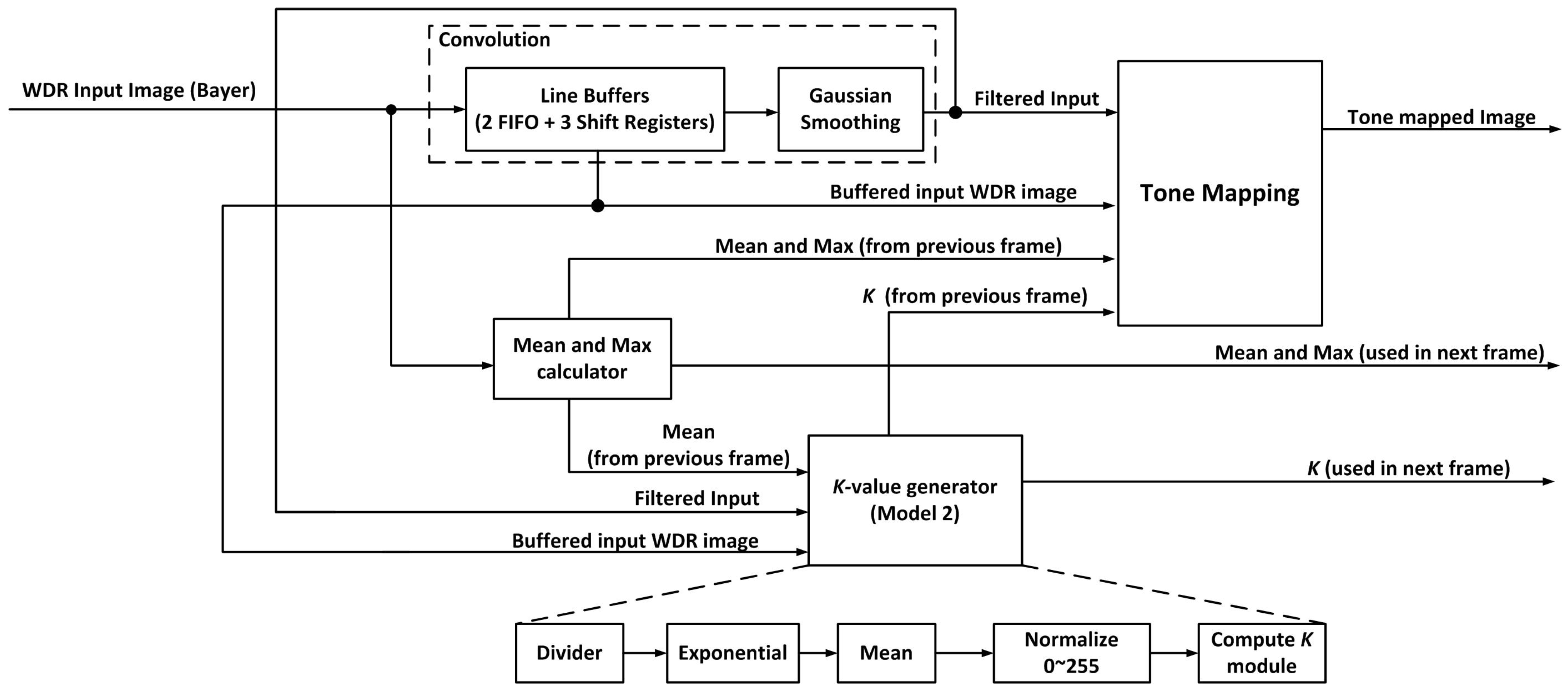
The actual tone mapping process is done on a pixel-by-pixel basis. First, a memory buffer is used to temporarily store the image; then, each pixel is continuously processed by the tone mapping system using modules that will be explained. The overview dataflow of the proposed tone mapping algorithm is described in Figure 10. The proposed tone mapping system contains five main modules: control unit, mean/max module, convolution module, factor k generator and inverse exponential module.

Figure 10. Dataflow chart for the hardware implementation of Glozman et al. [22,24].

Figure 10. Dataflow chart for the hardware implementation of Glozman et al. [22,24].

5.1. Convolution

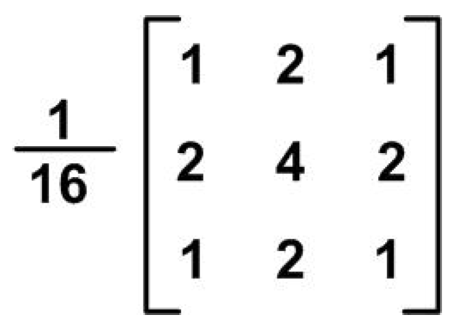
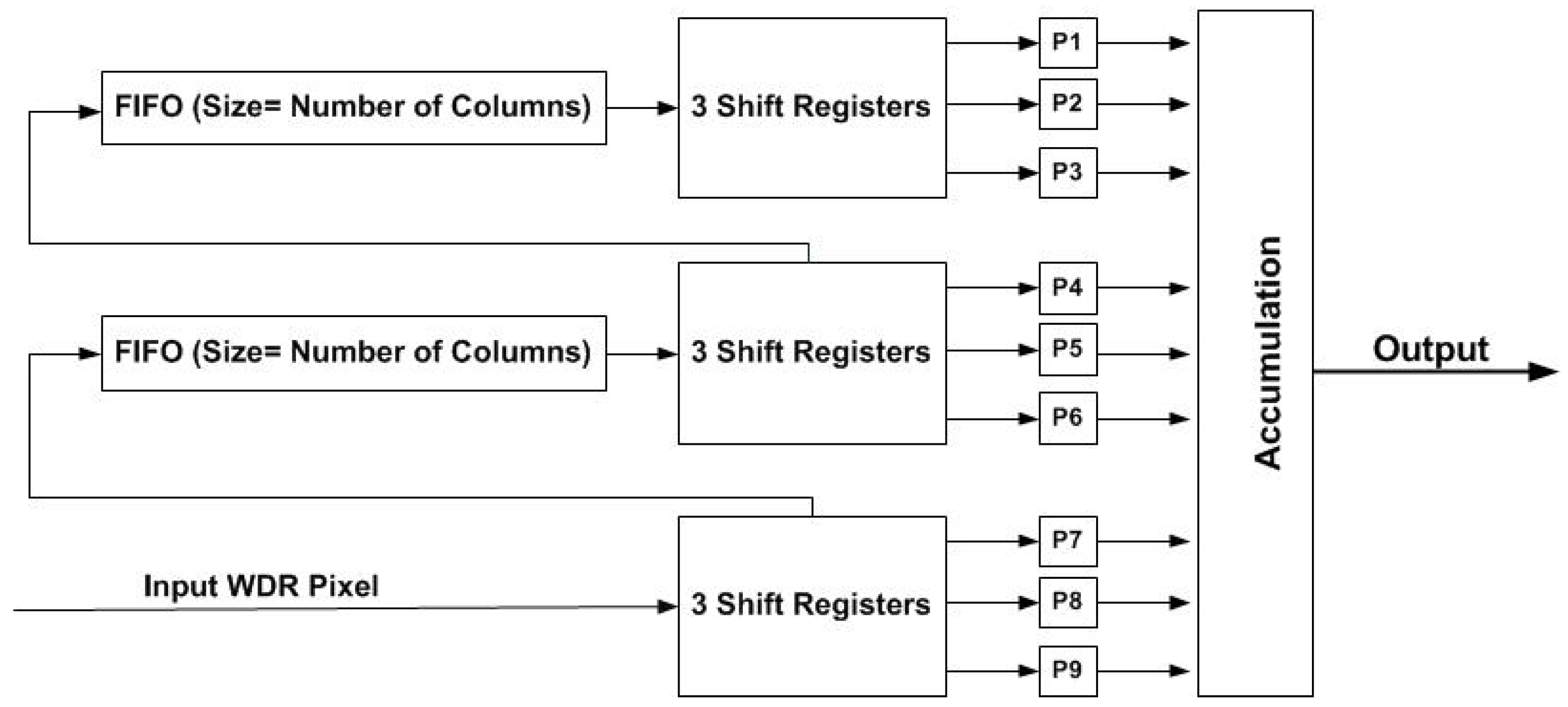
In this hardware design, a 3 × 3 convolution kernel is used for obtaining the information of the neighboring pixels (Figure 11). This simple kernel is used so that the output pixels can be calculated without the use of multipliers. The convolution module is divided into two modules; the 3 × 3 data pixel input generation module and the actual smoothing module. To execute a pipelined convolution, two FIFO and three shift registers are used [47,48]. The structure of the convolution module is shown in Figure 12. The two FIFO and the three three-bit-shift registers act as line buffers for the convolution module. The FIFO is used to store a row of the image frame. At every clock cycle, a new input enters the pixel input generation module via the three-bit-shift register, and the line buffers get systematically updated resulting in new 3 × 3 input pixels (P1–P9). These updated nine input pixels (P1–P9) are then used by the smoothing module for convolution computation with the kernel (Figure 11).

Figure 11. Simple Gaussian smoothing kernel used for implementing convolution.

Figure 11. Simple Gaussian smoothing kernel used for implementing convolution.

Figure 12. Convolution diagram for the field programmable gate array (FPGA).

Figure 12. Convolution diagram for the field programmable gate array (FPGA).

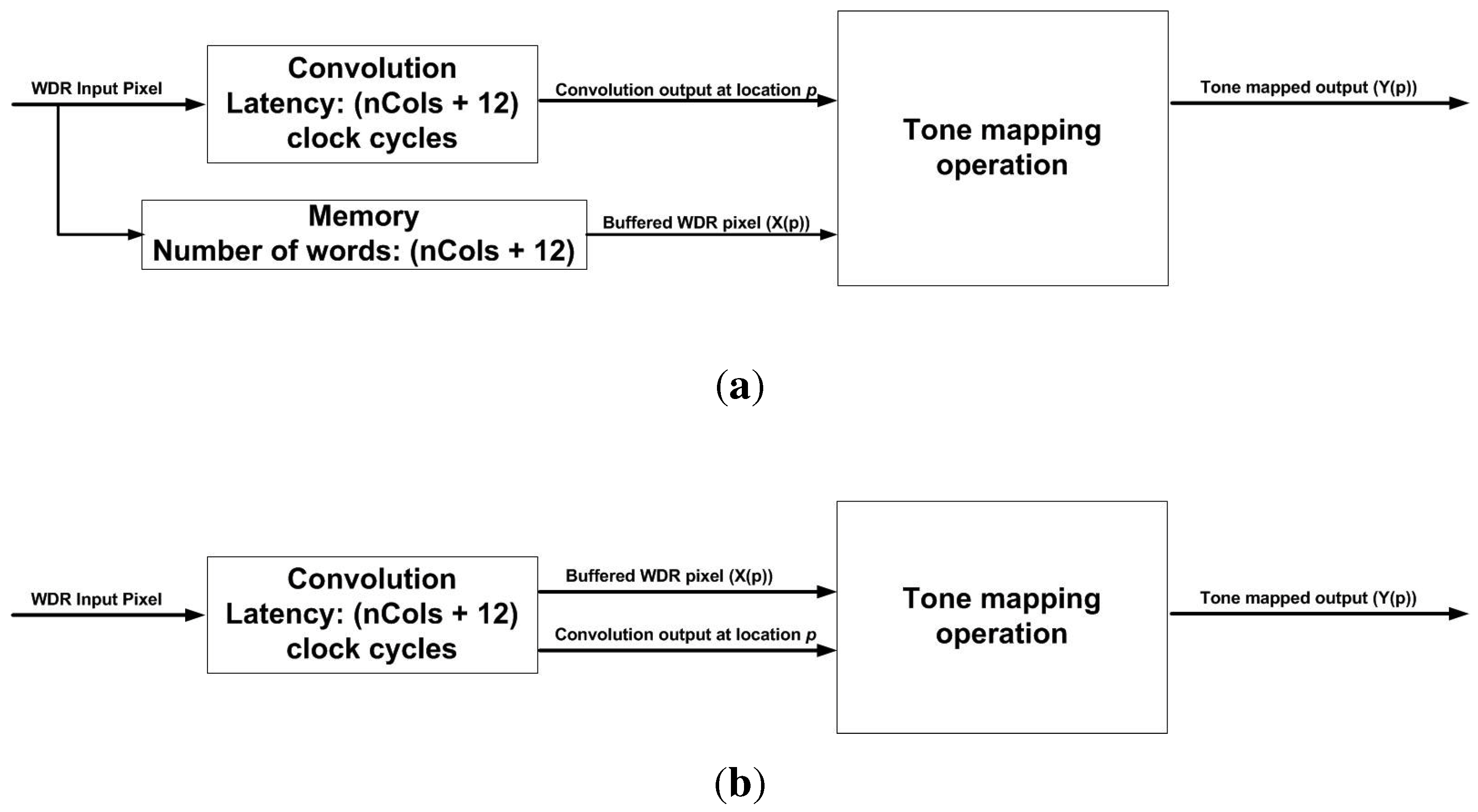
Inside the smoothing module, the output pixel is calculated by the use of simple adders and shift registers, thus removing the need for multipliers and dividers, which are expensive in terms of hardware resources. The convolution module has an initial latency of [number of pixel columns (nCols) + 12] clock cycles, because the FIFO buffers need to be filled before the convolution process can begin. This will result in the input pixel being stored in additional memory (FIFO), with the number of words being equal to the delay of the convolution system. To avoid this, the WDR input stored in the line buffer in the convolution module is used along with the convolution output of the same pixel location, for the actual tone mapping process in order to compensate for the delay, as well as to ensure that a pixel by pixel processing is maintained. Figure 13 shows a visual description of the readout system. The implemented approach is favorable for system-on-a-chip design, where the output from the CMOS image sensor can only be readout once and sent into the tone mapping architecture, thus saving memory, silicon area and power consumption.

Figure 13. (a) The implemented method of convolution and tone mapping operation, so as to reduce memory requirements; (b) the alternative method for the tone mapping architecture.

Figure 13. (a) The implemented method of convolution and tone mapping operation, so as to reduce memory requirements; (b) the alternative method for the tone mapping architecture.

5.2. Factor k Generator

There are three regions (A,B,C) in all of the proposed method for estimating the value of k needed for tone mapping a specific WDR image [Equation (7)]. Region A and B are both constants that are represented in fixed-point in the hardware design. Since region B of the k-equation is a power function with a base of two and a decimal number as the exponent, a hardware approximation was implemented in order to achieve good accuracy for the computation of factor k in that region. The hardware modification is shown in Equation (8):

$$y=a·2^{bx}=a·2^{(I+F)}$$

(8)

where I and F are the integer and fractional parts of the value, $bx$. The multiplication by $2^I$ can be implemented using simple shift registers, so as to reduce hardware complexity. Since $2^F$ can be expressed in an exponential form as $e^{(ln2)F}$, the k-equation for region B becomes:

$$y=a·2^{(I+F)}=a·2^I·e^{(ln2)F}$$

(9)

An iterative digit-by-digit exponent operation for computing exponential function $e^{(ln2)F}$ in fixed point precision was used. A detailed explanation of this operation can be found in [35,49]. It utilizes only shift registers and adders in order to reduce the amount of hardware resources needed for implementing exponential functions. A summary of the process is described below:

For any value of $x\in [0,ln2)$, $y=e^{\left(x\right)}$ can be approximated by setting up a data set of $(x_i,y_i)$, where the initial values are $x_0=x$ and $y_0=1$. Both $x_i$ and $y_i$ are calculated using the equations displayed below:

$$y_i=e^{-x_i}·e^x$$

(10)

$$x_{i+1}=x_i-ln\left(b_i\right)$$

(11)

where $b_i$ is a constant that is equal to $1+s_i·2^{-i}$, and i ranges from zero to 11. $s_i$ is equal to zero or one, depending on the conditions shown in Equation (12).

$$s=\left\{\begin{array}{cc}1,\hfill & \text{if}{x}_i\ge ln(1+2^{-i})\hfill \\ 0,\hfill & \text{otherwise}\hfill \end{array}\right.$$

(12)

Since we are implementing 12 fractional bits for the system’s fixed-point precision, a 12 × 12-bit read-only memory (ROM) is used as the lookup table for obtaining $ln\left(b_i\right)$. $x_i$ and $y_i$ are computed repetitively using the conditions displayed in Equations (13) and (14).

$$y_{i+1}=\left\{\begin{array}{cc}(1+2^{-i})·y_i,\hfill & \text{if}s=1\hfill \\ y_i,\hfill & \text{otherwise}\hfill \end{array}\right.$$

(13)

$$x_{i+1}=\left\{\begin{array}{cc}{x}_i-ln(1+2^{-i}),\hfill & \text{if}s=1\hfill \\ x_i,\hfill & \text{otherwise}\hfill \end{array}\right.$$

(14)

A shift and add operation can be used in computing $y_{i+1}$ in Equation (13) when $s=1$. Notice that in Equation (10), when $x_i=0$, then $y_i=e^x$, which is the final exponential value, since in our case, it is $e^{(ln2)F}$, where $0\le Fln2<ln2$. Taking $x_0=F·ln2$, we can use the iteration method explained above to calculate the exponential part of the k-equation [Equation (9)]. The k value obtained is stored and used for the next frame tone mapping operation, so that the processing time is not increased due to the addition of a k-generator.

5.3. Inverse Exponential Function

The inverse exponential function is important for the tone mapping algorithm by Glozman et al. [22,24], and it is described in Chapter 2. A modification of the digit-by-digit algorithm for implementing exponential functions on hardware was made [35]. It is similar to the exponential operation described above; however, in this case, because the tone mapping algorithm is an inverse exponential function, we will require hardware dividers if the original digit-by-digit algorithm was implemented. This will increase the hardware complexity and latency of the system. Therefore, the digit-by-digit algorithm was modified to suit this application. The main part of the original algorithm that is needed for this module and the modification of the algorithm are described below. For any value of x, it can be represented as shown in Equation (15):

$$x=(I+f)·ln2$$

(15)

where I and f are the integer and fractional parts of the value, x. To obtain I and f, the equation is rearranged as described in Equation (16).

$$I+f=x·{log}_{2}e$$

(16)

Therefore, for any arbitrary value of $y=expx$, it can be represented using Equation (17):

$$y=e^x=e^{(I+f)·ln2}=e^{I·ln2+f·ln2}=2^I{e}^{f·ln2}$$

(17)

Shift operation is also used to implement $2^I$ in order to reduce the hardware complexity of the module. Since f is a fractional number that lies between zero and one, $f·ln2$ therefore ranges from zero to $ln2$. Then, the Taylor series approximation (18) of the exponential equation (until the third order) can be used to calculate $e^{f·ln2}$.

$$e^{f·ln2}=1+\frac{f·ln2}{1!}+\frac{{\left(f·ln2\right)}^2}{2!}+\frac{{\left(f·ln2\right)}^3}{3!}$$

(18)

Since the actual equation used in the tone mapping algorithm is actually in an inverse exponential-based form, the following assumptions were made, as shown in Equation (19).

$$y=1-e^{-x}=\left\{\begin{array}{cc}A,\hfill & \text{if}x\le 8\hfill \\ 1,\hfill & \text{if}x>8\hfill \end{array}\right.$$

(19)

where $A=1-2^{-I}·e^{-f·ln2}$. The assumption in Equation (19) was made because $e^{-9}=0.00012341$, which is less than the quantization error of using 12 fractional bits for the tone mapping architecture ($0.00024414$). Using the Taylor series approximation of the equation $e^{-f·ln2}$ and the conditions in Equation (19), the overall equation is displayed below:

$$y=1-e^{-x}=\left\{\begin{array}{cc}1-\left[2^{-I}\times \left(1-\frac{f·ln2}{1!}+\frac{{\left(f·ln2\right)}^2}{2!}-\frac{{\left(f·ln2\right)}^3}{3!}\right)\right],\hfill & \text{if}x\le 8\hfill \\ 1,\hfill & \text{if}x>8\hfill \end{array}\right.$$

(20)

The hardware implementation of the inverse exponential function was performed in a pipelined manner, so as to facilitate the per pixel processing of the WDR image. The latency of the module is seven clock cycles.

5.4. Control Unit

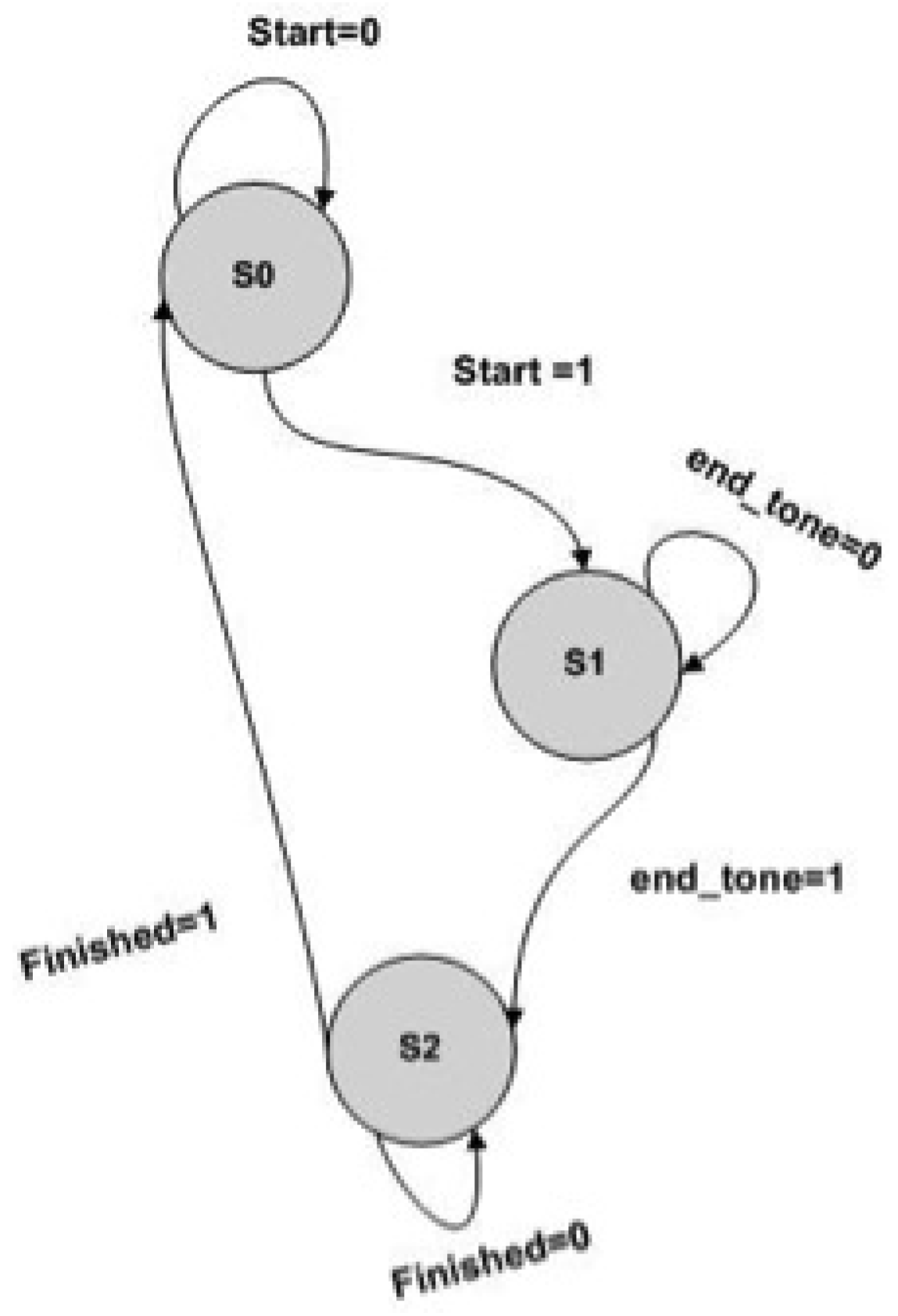
The control unit of the tone mapping system is implemented as finite state machines (FSM). It is used to generate the control signals to synchronize the overall tone mapping process (Figure 14). The operations and data flow of the whole tone mapping system is driven by the control unit.

The hardware implementation has three main states:

• S0: In this state, all modules remain inactive until the enable signal, Start, is set as high and the FSM moves to state S1;
• S1: In this state, the actual tone mapping operation is performed. An enable signal is sent to the external memory buffer, which results in one input WDR pixel being read into the system at each clock cycle. This input pixel is shared by the mean, maximum, factor k estimation block and image convolution. The input pixels from the frame buffer are used in computing the mean, maximum, factor k estimation block and image convolution. The filtered output values from the convolution module are used along with the input pixels for the actual computation of the tone mapping algorithm and the estimation of factor k. The mean, maximum and factor k of the previous frame are used in current frame tone mapping computation. Once all four computations have been completed and stored, an enable signal, endtone, is set high, and the FSM moves to state S2;
• S2: In this state, the mean, maximum and factor k of the current WDR frame are stored for the next frame image processing. An end signal, finished, is set high, and the FSM returns to state S0. The whole operation is repeated if there is another WDR frame to be processed.

Figure 14. State diagram of the controller for the tone mapping system.

Figure 14. State diagram of the controller for the tone mapping system.

In order to implement the system efficiently, all of the modules were executed in a pipelined and parallel manner. In total, four dividers were used in the design in which three dividers were 44 bits long and one divider was a 14-bit word length for the fixed point division. A more descriptive image of the processing stages involved in the hardware design implemented is shown in Figure 15 and Figure 16.

Figure 15. Diagram of the pathway of the input in the hardware implementation of the tone mapping system.

Figure 15. Diagram of the pathway of the input in the hardware implementation of the tone mapping system.

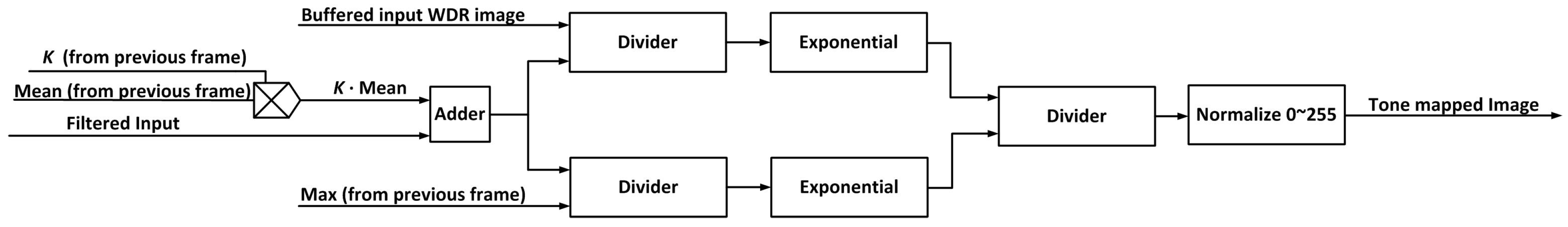
Figure 16. Detailed diagram of the pathway for the tone mapping operation in hardware.

Figure 16. Detailed diagram of the pathway for the tone mapping operation in hardware.

It should be noted that the mean and maximum values of the current frame are stored for processing the next frame, while the mean and maximum values of the previous frame are used in the tone mapping operation of the present frame. Since the k computation also requires the mean of the compressed image frame, the k value of a previous frame can be used. This is because when operating in real-time, such as 60 fps, there are very little variations in information from one frame to the next [50]. This saves in terms of processing speed and removes the need to store the full image memory in order to calculate the mean and maximum and, then, implement the tone mapping algorithm. As a result, power consumption will also be reduced in comparison to a system that would have required the use of an external memory buffer for storing the image frame.

6. Experimental Results

WDR images from the Debevec library and other sources were used to test the visual quality of both hardware architectures. These WDR images were first converted to the Bayer CFA pattern on MATLAB^®. Then, the Bayer result was converted into fixed-point representation and used as an input into the hardware implementation of the tone mapping operator. The tone mapped output image was converted back to the RGB image format using a simple bilinear interpolation on MATLAB^®. Output images from functional simulation using ModelSim^® for WDR images are shown in Figure 17, Figure 18 and Figure 19.

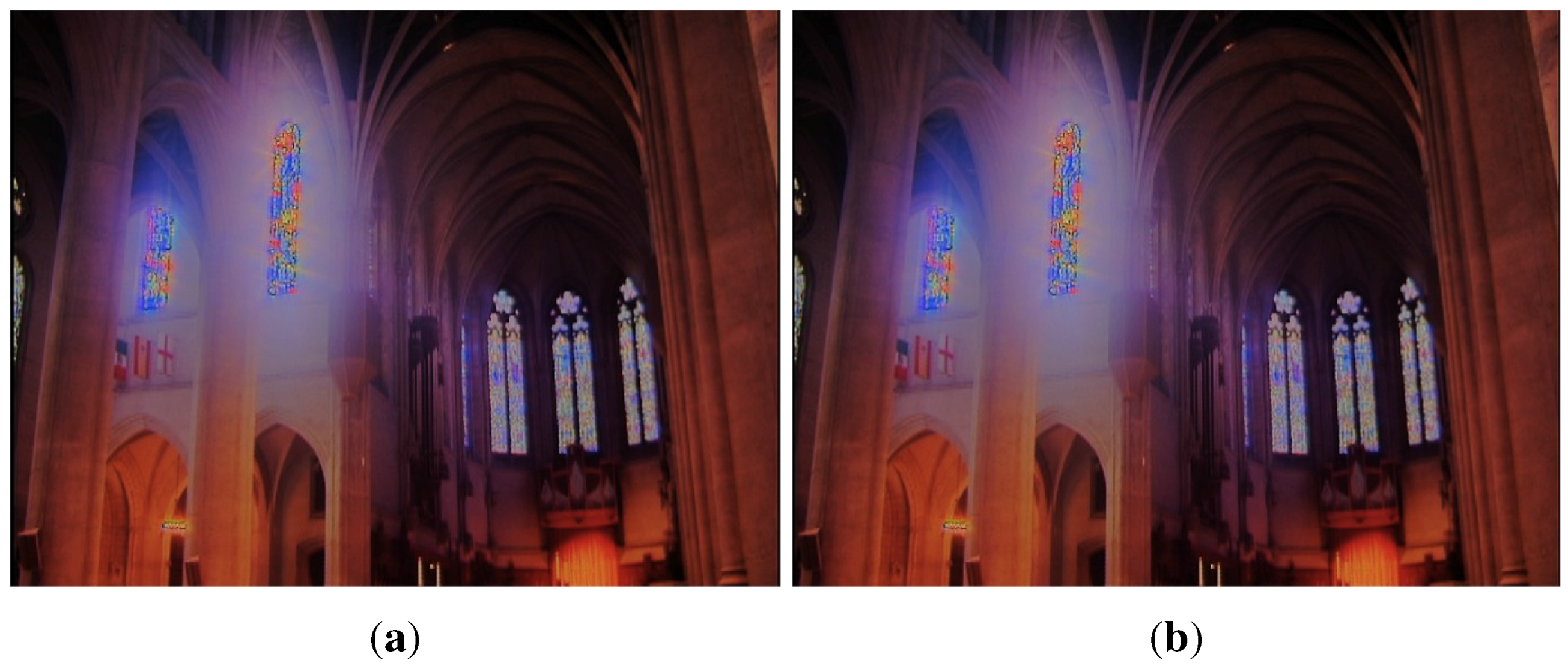
Figure 17. Nave image [image size (1024 × 768)] [51]. (a) Simulation results; (b) Hardware results.

Figure 17. Nave image [image size (1024 × 768)] [51]. (a) Simulation results; (b) Hardware results.

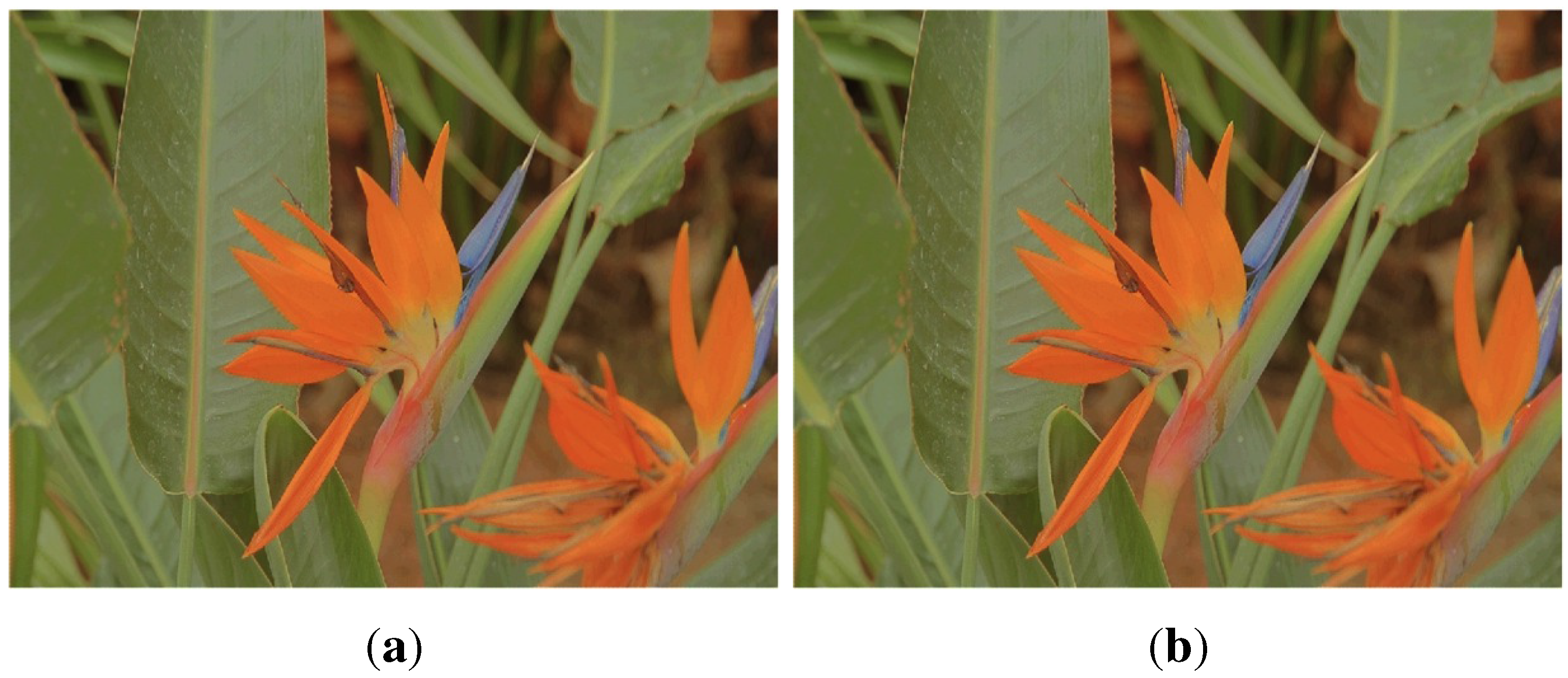
Figure 18. Bird of paradise image [image size (1024 × 768)] [29]. (a) Simulation results; (b) Hardware results.

Figure 18. Bird of paradise image [image size (1024 × 768)] [29]. (a) Simulation results; (b) Hardware results.

Figure 19. Raw image [image size (1152 × 768)]. (a) Simulation results; (b) Hardware results.

Figure 19. Raw image [image size (1152 × 768)]. (a) Simulation results; (b) Hardware results.

6.1. Image Quality: Peak Signal-to-Noise Ratio (PSNR)

The peak signal-to-noise ratio (PSNR) of the results from the hardware simulation on ModelSim^® was calculated in order to quantify the amount of error produced due to the use of fixed-point precision. The results from the floating point implementation on MATLAB^® were used in this quantitative evaluation. Using Equations (21) and (22), the PSNR was calculated:

$$PSNR=10{log}_{10}[\frac{{255}^2}{MSE}]$$

(21)

$$MSE=\frac{1}{MN}\sum _{m=0}^{M-1}\sum _{n=0}^{N-1}{\left[f\right(m,n)-k(m,n\left)\right]}^2$$

(22)

where MSE is the mean-squared error between the output images obtained from the floating point implementation and the fixed-point implementation on hardware. Higher PSNR values indicate better visual image similarity between the two images being compared. The PSNR values of implementations are shown in Table 3. It should be noted that the hardware-friendly approximations made while implementing the k generator module may have affected the PSNR of the tone-mapped images. Even with that, the results show that the hardware implementation of the tone mapping algorithm produce acceptable results that can be compared to the MATLAB^® simulations.

Table 3. peak signal-to-noise ratio (PSNR) of images tested.

Image (N × M)	Implementation PSNR (dB)
Nave (720 × 480)	56.11
Desk (874 × 644)	46.21
Bird of Paradise (1024 × 768)	49.63
Memorial (512 × 768)	54.27
Raw Image (1152 × 768)	54.85

Table 3. peak signal-to-noise ratio (PSNR) of images tested.

Image (N × M)	Implementation PSNR (dB)
Nave (720 × 480)	56.11
Desk (874 × 644)	46.21
Bird of Paradise (1024 × 768)	49.63
Memorial (512 × 768)	54.27
Raw Image (1152 × 768)	54.85

6.2. Image Quality: Structural Similarity (SSIM)

SSIM is an objective image quality assessment tool that is used for measuring the similarity between two images [52]. The SSIM index obtained is used to evaluate how one image is structurally similar to another image that is regarded as perfect quality. Using Equation (23), the SSIM was calculated [52]:

$$SSIM=\frac{\left(2{\mu }_x{\mu }_y+C_1\right)\left(2{\sigma }_{xy}+C_2\right)}{\left({{\mu }_x}^2+{{\mu }_y}^2+C_1\right)\left({{\sigma }_x}^2+{{\sigma }_y}^2+C_2\right)}$$

(23)

where x and y represent two image patches obtained from the same spatial location in the two images being compared. The mean of x and the mean of y are represented by ${\mu }_x$ and ${\mu }_y$, respectively. The covariance of x and y is represented by ${\sigma }_{xy}$. The variance of x and the variance of y are denoted by ${\sigma }_x^2$ and ${\sigma }_y^2$, respectively. The variances are used to interpret the contrast of the image, while the mean is used to represent the luminance of the image [52]. The constants, $C_1$ and $C_2$, are used to prevent instability in the division. They are calculated based on Equations (24) and (25):

$$C_1={(K_1·L)}^2$$

(24)

$$C_2={(K_2·L)}^2$$

(25)

where L is the dynamic range of the pixel values (255- for eight-bit tone-mapped images). $K_1$ and $K_2$ are $0.01$ and $0.03$, respectively. The closer the SSIM values are to one, the higher the structural similarity between the two images being compared. The SSIM values of images are shown in Table 4.

Table 4. Structural similarity (SSIM) of the images tested.

Image (N × M)	Implementation SSIM
Nave (720 × 480)	0.9999
Desk (874 × 644)	0.9998
Bird of Paradise (1024 × 768)	0.9998
Memorial (512 × 768)	0.9998
Raw image (1152 × 768)	0.9997

Table 4. Structural similarity (SSIM) of the images tested.

Image (N × M)	Implementation SSIM
Nave (720 × 480)	0.9999
Desk (874 × 644)	0.9998
Bird of Paradise (1024 × 768)	0.9998
Memorial (512 × 768)	0.9998
Raw image (1152 × 768)	0.9997

6.3. Performance Analysis: Hardware Cost, Power Consumption and Processing Speed

The FPGA implementation of the overall system was evaluated in terms of the hardware cost, power consumption and processing speed. In Table 5, a summary of the synthesis report from Quartus v11.1 for the Stratix II and Cyclone III devices is shown for the architecture. The system was designed in such a way that the total number of logic cells and registers used would not dramatically increase if the size of the image became greater than 1024 × 768. However, the number of memory bits would increase because of the two-line buffers used in the convolution module.

In addition, since power consumption is of importance for possible applications, such as mobile devices and still/video cameras, ensuring that the system consumes low power is of great importance. Using the built in PowerPlay power analyzer tool of Altera^® Quartus v11.1, the power consumption of the full tone mapping system was estimated for the Cyclone III device. The power consumed by the optimized tone mapping system when operating at a clock frequency of 50 MHz was estimated to be 250 mW.

Table 5. FPGA synthesis report for a 1024 × 768 multi-fused WDR image.

Stratix II EP2S130F780C4	Used	Available	Percentage (%)
Combinatorial ALUTs	8,546	106,032	8.06
Total registers	10,442	106,032	9.85
DSP block nine-bit elements	60	504	11.90
Memory bits	68,046	6,747,840	1.00
Maximum frequency (MHz)	114.90	N/A	N/A
Operating frequency (MHz)	50	N/A	N/A
Cyclone III EP3C120F48417	Used	Available	Percentage (%)
Combinatorial functions	12,154	119,088	10.21
Total registers	10,518	119,088	8.83
Embedded multipliers nine-bit elements	36	576	6.25
Memory bits	68,046	3,981,312	1.71
Maximum frequency (MHz)	116.50	N/A	N/A
Operating frequency (MHz)	50	N/A	N/A

Table 5. FPGA synthesis report for a 1024 × 768 multi-fused WDR image.

Stratix II EP2S130F780C4	Used	Available	Percentage (%)
Combinatorial ALUTs	8,546	106,032	8.06
Total registers	10,442	106,032	9.85
DSP block nine-bit elements	60	504	11.90
Memory bits	68,046	6,747,840	1.00
Maximum frequency (MHz)	114.90	N/A	N/A
Operating frequency (MHz)	50	N/A	N/A
Cyclone III EP3C120F48417	Used	Available	Percentage (%)
Combinatorial functions	12,154	119,088	10.21
Total registers	10,518	119,088	8.83
Embedded multipliers nine-bit elements	36	576	6.25
Memory bits	68,046	3,981,312	1.71
Maximum frequency (MHz)	116.50	N/A	N/A
Operating frequency (MHz)	50	N/A	N/A

For the hardware architecture, the maximum frequency obtained for the Stratix II and Cyclone III were 114.90 MHz and 116.50 MHz, respectively. In order to calculate the processing time for one N × M pixel resolution, Equation (26) is used.

$$T=\left[\text{Total}\text{clock}\text{cycles}\text{per}\text{frame}\right]·\frac{1}{\text{operating}\text{clock}\text{frequency}}$$

(26)

$$\text{Total}\text{clock}\text{cycles}\text{per}\text{frame}=M·N+N+100$$

(27)

This implies that for a 1024 × 768 image using this hardware implementation, the processing time for tone mapping of each frame is 7.9 ms (126 fps) and 3.45 ms (63 fps) at a clock frequency of 100 MHz and 50 MHz, respectively. This means that the system can work in real-time if the input video rate is 60 fps at a lower clock frequency of 50 MHz.

6.4. Comparison with Existing Research

In Table 6, a comparison of the proposed tone mapping architecture with other tone mapping hardware systems in terms of processing speed, logic elements, memory, power consumption and PSNR is shown. All the FPGA-based (Altera^®) systems compared utilized a Stratix II device. Due to proprietary reasons, there is no way of converting the hardware resources requirements for the Xilinx^®-based tone mapping system by Ureña et al. [25,37] to an Altera^® system. In this case, only properties, such as memory requirements, power consumption and processing speed, are compared with the other hardware-based systems.

The proposed full tone mapping system utilizes less hardware resources (logic elements and memory) in comparison to the other hardware tone mapping systems published. This is because of the low complexity of implementing the automatic rendering algorithm and tone mapping algorithm, since they are both exponent-based functions. In addition, proposed hardware architecture achieves higher and similar processing times in comparison to the other hardware-based systems implemented. Furthermore, the power consumption estimated for the proposed tone mapping algorithm using the Quartus power analyzer was lower in contrast to the only found power results for a tone mapping system implemented on an FPGA. Ureña et al.’s hardware architecture consumed 4× more power in contrast to our systems that implemented a larger image size (1024 × 768). Taking into account that if we implement our full tone mapping algorithm in ASIC rather than FPGA [53], our power consumption is anticipated to decrease substantially. Thus, we can conclude that our system achieves our goals of being low power-efficient.

It should be noted that among the hardware systems compared, only this current hardware architecture implements a rendering parameter selection unit that automatically adjusts the rendering parameter’s value based on the properties of the image being processed. Hassan et al. [33], Carletta et al. [34] and Vylta et al. [36] selected a constant value for their rendering parameters, while Chiu et al. [35] and Ureña et al. [25] required the manual adjustment of their rendering parameters. This is not favorable for a real-time video processing applications, where the parameters need to be constantly adjusted or a constant value may not work for varying image key.

Table 6. Comparison with other tone mapping hardware implementation. (fps: frames per second; SOC: system-on-a-chip).

Research Works	Tone mapping algorithm	Type of tone mapping operator	Design Type	Frame size	Image type	Maximum operating frequency (MHz)	Processing speed (fps)	Logic elements	Memory (bits)	Power (mW)	PSNR (dB) (memorial image)
This work	Improved Glozman et al. [22,24]	Global and local	FPGA (Altera)	1,024 × 768	Color	114.90	126	8,546	68,046	250	54.27
Hassan et al. [33]	Reinhard et al. [18]	Local	FPGA (Altera)	1,024 × 768	Monochrome	77.15	60	34,806	3,153,408	N/A	33.70
Carletta et al. [34]	Reinhard et al. [18]	Local	FPGA (Altera)	1,024 × 768	Color	65.86	N/A	44,572	3,586,304	N/A	N/A
Vylta et al. [36]	Fattal et al. [26]	Local	FPGA (Altera)	1 Megapixel	Color	114.18	100	9,019	307,200	N/A	53.83
Chiu et al.[35]	Reinhard et al. [18]/ Fattal et al. [26]	Global / Local	ARM-SOC	1,024 × 768	N/A	100	60	N/A	N/A	177.15	45/35
Ureña et al. [25,37]	Ureñaet al. [25,37]	Global and local	FPGA (Xilinx)	640 × 480	Color	40.25	60	N/A	718,848	900	N/A

Table 6. Comparison with other tone mapping hardware implementation. (fps: frames per second; SOC: system-on-a-chip).

Research Works	Tone mapping algorithm	Type of tone mapping operator	Design Type	Frame size	Image type	Maximum operating frequency (MHz)	Processing speed (fps)	Logic elements	Memory (bits)	Power (mW)	PSNR (dB) (memorial image)
This work	Improved Glozman et al. [22,24]	Global and local	FPGA (Altera)	1,024 × 768	Color	114.90	126	8,546	68,046	250	54.27
Hassan et al. [33]	Reinhard et al. [18]	Local	FPGA (Altera)	1,024 × 768	Monochrome	77.15	60	34,806	3,153,408	N/A	33.70
Carletta et al. [34]	Reinhard et al. [18]	Local	FPGA (Altera)	1,024 × 768	Color	65.86	N/A	44,572	3,586,304	N/A	N/A
Vylta et al. [36]	Fattal et al. [26]	Local	FPGA (Altera)	1 Megapixel	Color	114.18	100	9,019	307,200	N/A	53.83
Chiu et al.[35]	Reinhard et al. [18]/ Fattal et al. [26]	Global / Local	ARM-SOC	1,024 × 768	N/A	100	60	N/A	N/A	177.15	45/35
Ureña et al. [25,37]	Ureñaet al. [25,37]	Global and local	FPGA (Xilinx)	640 × 480	Color	40.25	60	N/A	718,848	900	N/A

7. Conclusions

In this paper, we proposed an algorithm that can be used in estimating the rendering parameter k, needed for Glozman et al.’s operator. The automatic rendering algorithm requires the image statistics of the WDR image in order to determine the value of the rendering parameter k that will be used. An approximation of the independent property of the WDR image is obtained by initially compressing the WDR image in order to have a standard platform for obtaining the rendering parameter for different WDR images. This compressed image is not used for the actual tone mapping process by Glozman et al.’s operator, and it is mainly for configuration purposes. Hence, no additional memory is needed for storing the initial compressed image frame. The proposed algorithm was able to estimate the rendering parameter k that was needed for tone mapping a variety of WDR images.

A hardware-based implementation of the automatic rendering algorithm along with Glozman et al.’s tone mapping algorithm was also presented in this paper. The hardware architecture produced output images with good visual quality and high PSNR and SSIM values in comparison to the compressed images obtained from the software simulation of the tone mapping system. The hardware implementation produced output images in Bayer CFA format that can be converted to an RGB color image by using simple demosaicing techniques on hardware. Low hardware resources and power consumption were also achieved in comparison to other hardware-based tone mapping systems published. WDR images were processed in real-time, because of approximations made when designing the hardware architecture. Potential applications, such as medical imaging, mobile phones, video surveillance systems and other WDR video applications, will benefit from a real-time embedded device with low hardware resources and automatic configuration.

The overall architecture is well compacted, and it does not require the constant tuning of the rendering parameters for each WDR image frame. Additionally, it requires low hardware resources and no external memory for storing the full image frame, thereby making it adequate as a part of a system-on-a-chip. Future research may concentrate on embedding the tone mapping system as a part of a system-on-a-chip with WDR imaging capabilities. In order to achieve this, the WDR image sensor should also have an analog-to-digital converter (ADC) as part of the system. In addition, characteristics of the automatic generation of the rendering parameter k with respect to flickering artifacts during WDR video compression should be investigated in future works.