Article

Artificial Crab Burrows Facilitate Desalting of Rooted Mangrove Sediment in a Microcosm Study

1
Leibniz Center for Tropical Marine Ecology (Leibniz-ZMT), Fahrenheitstr. 6, Bremen 28359, Germany
2
Edinburgh Napier University, School for Life, Sport and Social Sciences, Edinburgh EH11 4BN, UK
3
Laboratório de Botânica, Universidade Federal do Pará, Campus Bragança, Alameda Leandro Ribeiro s/n, Bragança-Pará, CEP 68600-000, Brazil
*
Author to whom correspondence should be addressed.
These authors contributed equally to this work.
J. Mar. Sci. Eng. 2015, 3(3), 539-559; https://doi.org/10.3390/jmse3030539
Submission received: 1 June 2015 / Accepted: 3 July 2015 / Published: 15 July 2015
(This article belongs to the Special Issue Biogeochemical Cycles in Mangrove Forests)

Abstract

:
Water uptake by mangrove trees can result in salt accumulation in sediment around roots, negatively influencing growth. Tidal pumping facilitates salt release and can be enhanced by crab burrows. Similarly, flushing of burrows by incoming tidal water decreases sediment salinity. In contrast to burrows with multiple entrances, the role of burrows with one opening for salinity reduction is largely unknown. In a microcosm experiment we studied the effect of artificial, burrow-like macro-pores with one opening on the desalting of mangrove sediment and growth of Rhizophora mangle L. seedlings. Sediment salinity, seedling leaf area and seedling growth were monitored over six months. Artificial burrows facilitated salt release from the sediment after six weeks, but seedling growth was not influenced. To test whether crab burrows with one opening facilitate salt release in mangrove forests, sediment salinities were measured in areas with and without R. mangle stilt roots in North Brazil at the beginning and end of the wet season. In addition, burrows of Ucides cordatus were counted. High crab burrow densities and sediment salinities were associated with stilt root occurrence. Precipitation and salt accumulation by tree roots seem to have a larger effect on sediment salinity than desalting by U. cordatus burrows.

1. Introduction

Mangrove trees are typically exposed to saline tidal waters. Most mangrove species are able to exclude salt during water uptake and/or to regulate ion concentration via salt glands [1,2]. The drawback of excluding salt during water uptake is the consequential accumulation of salt in the sediment surrounding the roots [3]. Under poorly flushed conditions, the accumulated salt around the roots may reach concentrations that limit further water uptake, leading, in the worst case, to lethal conditions for the tree [3]. Moreover, mangrove sediments usually feature a high proportion of clay or silt with low hydraulic conductivity and low diffusion coefficients for salt [4,5,6], resulting in low diffusion rates and thereby a slow removal of accumulated salt by groundwater flow [7].
Salt can be washed out by tidal pumping [8,9] or by tidal flushing of animal burrows [10,11,12]. Tidal pumping (tidally driven pore or groundwater flow) is the infiltration of seawater into the sediment during flood tides and the discharge of groundwater during ebb tides [13,14,15]. During this process, nutrients, dissolved organic carbon, and salt enter and seep out of the sediment [9,16,17,18,19,20,21]. The effects of tidal pumping can be intensified by the presence of animal burrows [8,19,22,23]. During tidal flushing, tidal waters mix with the water inside the burrows; in the case of burrows with more than one opening, a tidally driven water circulation through burrows may result [8,24,25].
Burrowing crabs are abundant in mangrove ecosystems [26]; their burrows increase the sediment surface area [27] where exchange processes with air or water take place [28]. The extent to which these exchange processes are influenced by the presence of burrows will depend, among others, on the burrow morphology, which affects, in particular, tidal flushing. Different burrow morphologies are (i) burrows with one opening (from here on referred to as “simple burrows”), (ii) U-shaped and multiple-looped burrows with two openings and (iii) complex burrows with more than two openings [10,12,29,30]. The mechanism of tidal flushing in burrows with only one opening under natural conditions is not well understood. In contrast, to date U-shaped and multiple-looped burrows are the most studied burrow types in terms of tidal flushing [10,11,12,24,25]. Tidal flushing of U-shaped and multiple-looped burrows can facilitate salt release from the sediment as it enhances salt diffusion from salt-enriched sediment pore water to lower concentrated burrow water. The salt can then be flushed out during the next flood tide [10,11,12]. The rate of tidal flushing through U-shaped crab burrows in an Australian mangrove forest (0.01–0.04 m3 m−2 day−1) was quantitatively similar to the rate of tidally driven groundwater flow (0.004–0.04 m3 m−2 day−1) indicating that this type of burrow significantly enhances the water flow in mangrove sediments [15].
The formerly investigated U-shaped and multiple-looped burrows belonged mainly to Sesarmid crabs from the Indo-West Pacific region. Mangroves of the Atlantic-East Pacific are dominated by Ocypodid crabs; these crabs build usually burrows with one opening. In Brazil, the abundant large mangrove crab Ucides cordatus (Ucididae) constructs burrows with mainly one opening to depths of 55–211 cm [31]. Their average density is 1.7 ind. m−2 for a Rhizophora mangle L. (Rhizophoraceae) dominated forest in North Brazil [32], and a maximal carapace width of 10 cm was recorded [33]. Ucides cordatus prefers to build its burrows close to stilt roots of R. mangle trees, probably because the roots increase sediment stability and provide shelter against predators [34]. Roots of R. mangle trees can reach depths of 200 cm [2], but the main bulk of living roots is concentrated in the upper sediment layer down to a depth of 50 cm [35]. Ucides cordatus burrows therefore extend over the whole depth range of the possible root distribution. Given that U. cordatus constructs its burrows preferably in the vicinity of R. mangle roots, and thus in the zone of salt accumulation [3], it is an intriguing question whether tidal pumping or flushing of the crabs’ burrows significantly removes excess salt accumulated by the trees’ root system. If a significant removal of salt took place, burrowing activity by U. cordatus would be likely to improve growth conditions for the mangrove trees by maintaining root space salinity at tolerable limits.
Besides U. cordatus, Ocypodid fiddler crabs (Uca spp.) are also abundant in Brazilian mangrove forests (28–105 burrows m−2, own data). Fiddler crabs construct shallower burrows than U. cordatus, but likewise with one opening (e.g., Uca maracoani constructs burrows of 20–40 cm depth, [36]). As fiddler crabs feed on microphytobenthos and microheterotrophs [37,38,39,40], they prefer areas with a less dense canopy. Therefore, they are not as closely associated with roots as U. cordatus burrows, hence, those crabs were not considered further in this study.
The objective of this study was to investigate the effect of artificial crab burrows with one opening on the desalting of the sediment and a possible positive effect of the desalting on seedling growth. Therefore, we established a greenhouse microcosm experiment growing R. mangle seedlings under simulated, regular tidal inundation, monitoring sediment salinity and plant development in treatments with and without artificial macro-pores modeled after crab burrows. The hypotheses of this study are that (a) artificial burrows decrease salt accumulation resulting in lower sediment salinities and (b) desalting of sediment would increase seedling growth measured as increase of total leaf area and of shoot length and dry biomass of leaves, stem/branches and roots between the first and the last sampling date. Further, sediment salinities and U. cordatus burrow density in rooted areas (high concentration of R. mangle stilt roots) and non-rooted gaps (between trees) were determined in a R. mangle forest to study the desalting effect of burrows. It was hypothesized that (c) areas with high burrow densities presented lower sediment salinities than areas with low burrow densities.

2. Experimental Section
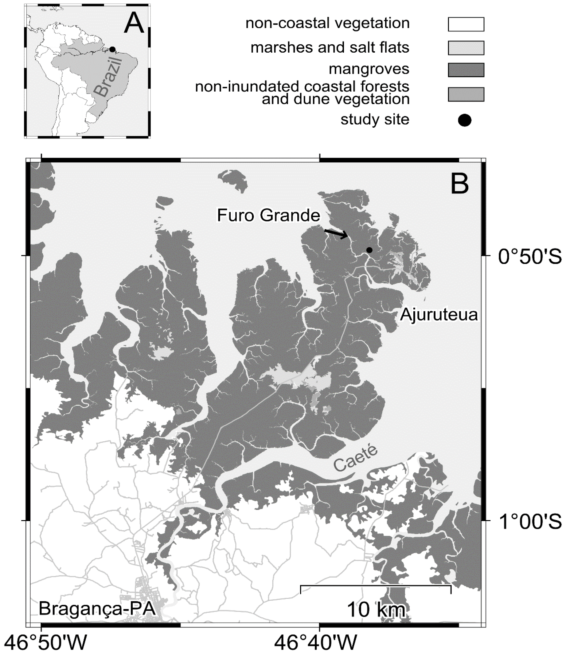
2.1. Study Area

The microcosm experiment was conducted in a greenhouse on the campus of the Federal University of Pará (UFPA), Bragança, Pará state, North Brazil (Figure 1). Field work was conducted in the Caeté estuary, approximately 30 km northwest of the city of Bragança, in an intertidal mangrove forest near the tidal channel Furo Grande (46°38′ W 0°50′ S, Figure 1B). The mangrove forest is dominated by R. mangle trees [41]. Tides are semidiurnal and tidal amplitude ranges between 3 and 5 m. Most of the Caeté mangrove forest, including the sampling site, is located in the high intertidal zone and is therefore not flooded during neap high tides. Mean annual temperature and precipitation for 2010–2012 recorded at the weather station of Tracuateua, 50 km from the study area, were 26.4 °C and 2054 mm, respectively [42]. Rainfall is seasonal, with a wet season from January to August and a dry season (monthly precipitation <100 mm) from September to December [42].
Figure 1. Study area (46°38′ W 0°50′ S) in Northern Brazil (A) near the city of Bragança on the Ajuruteua peninsula on the western bank of the Caeté estuary (area within the black dot). The study site is marked by a black dot and lies at the tidal channel Furo Grande (B).
Jmse 03 00539 g001

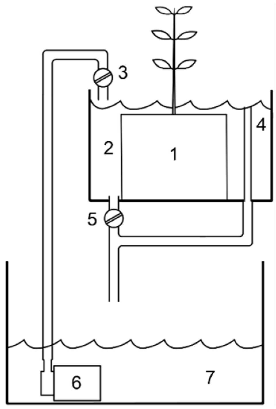
2.2. Microcosm Experiment

Rooted R. mangle seedlings with 3 to 4 pairs of leaves were collected from a mangrove forest next to the tidal channel Furo Grande in November 2012. To minimize damage to the root system, care was taken to extract and transport the plants with intact root balls (diameter about 25 cm) surrounded by natural substrate. In the greenhouse, the seedlings were carefully replanted into perforated plant containers with 23 cm high and 40 cm wide; the diameter of perforations was 3 cm. Intertidal surface sediment excavated from a depth of up to 30 cm (collected at a neighboring channel close to Furo Grande) was added around the root ball.
Plant containers were wrapped from the outside with a 0.5 cm thick felt layer and a 3 cm thick open cell foam sheet to prevent the sediment within the containers from being washed out through the perforations. Plant containers were placed into 60 × 60 cm open tanks with 30 cm height. Each tank was connected to the main water reservoir with an adjustable water inlet, a spillway tube and an adjustable water outflow. The water reservoir was filled with natural seawater (salinity 32 ppt) from Furo Grande; its pH was stabilized by establishing a bicarbonate buffering system with marble stone fragments in the reservoir. During periods of tidal inundation, electrical centrifugal aquarium pumps slowly circulated the seawater between the tanks and the water reservoir (Figure 2). A timer regulated the flooding of the tanks. Using the height of the spillway tube, four different tidal inundation levels were regulated during the experiment (described below). Tanks were shaded with perforated gauze (experimental design adapted from [43]).
Figure 2. Schematic drawing of one section of the experimental microcosm setting with (1) an experimental seedling in its container, placed into (2) a tank. Altogether there were 18 tanks. Tanks had (3) an adjustable water inlet, (4) a spillway tube and (5) an adjustable water outflow. The adjustable water outflow regulated the artificial tiding between spring tide (as shown in drawing: 25 cm, 3 days), intermediate level 2 (18.5 cm, 2 days), intermediate level 1 (12 cm, 2 days) and neap tide (5.5 cm, 3 days). Water was pumped to the tanks with (6) electrical centrifugal aquarium pumps from (7) a water reservoir filled with natural seawater (salinity: 32 ppt).
Jmse 03 00539 g002
Plants were acclimated for three months. Within this time period, plant containers were maintained completely flooded (inundation level: 25 cm) from 6 am to 6 pm (light phase) to wash excess salt from the sediment and to prevent evaporation at the sediment surface. Water was released overnight to let the sediment dry without the influence of desiccation by the sun.
To simulate spring and neap tides, tanks were flooded to a height of 25 cm and 5.5 cm above the tank floor, respectively. To better simulate natural flooding conditions, two intermediate tidal levels were implemented between spring and neap tide with water heights of 12 cm (intermediate level 1) and 18.5 cm (intermediate level 2).
Water salinity, pH and temperature in the water reservoir were measured daily in the evening using a WTW TetraCon 325 and a WTW Sentix 41 pH-electrode connected to a WTW portable meter (Multi 340i, Geotech, Weilheim, Germany), respectively. Water pH ranged between 7.7 and 8.3 and water temperature varied between 26 °C and 33 °C. Prior to the first sampling, seawater (salinity: 32 ppt) was added to the reservoir. During the experiment fresh water from the tap or seawater was added when salinity was higher or lower than 32 ppt, respectively. Higher amounts of seawater were also regularly (daily to weekly) added to the water reservoir when significant amounts of water had evaporated. The large size of the water reservoir (3000 L), the frequent addition of fresh sea- or tap water and the relatively short duration of the experiment (6 months) minimized the risk of nutrient depletion.

2.3. Microcosm Sampling

After three months of acclimation, plant containers (n = 18) were randomly assigned to one of two treatments (burrow and control) to test the effect of artificial macro-pore (“crab burrows”) on sediment salinity and R. mangle seedling growth. By using artificial burrows, we were able to maintain constant burrow dimension and position across replicates. For the burrow treatment, four vertical holes (3.5 cm diameter, 20 cm depth) were cored into the substrate with a plastic tube. The selected burrow size is smaller than that of average burrows of adult U. cordatus crabs and was chosen as a compromise between realistically simulating the field conditions and maintaining the size of the microcosm within technically feasible dimensions. The four holes were regularly distributed in a circle around the seedlings at a distance of 10 cm from the stem. Holes were re-cored weekly to simulate maintenance by the crab. No holes were cored in the sediment of the control treatment.
Plant containers were flooded for 6 hours twice a day simulating high and low tide. To simulate natural tidal conditions one spring-neap tide cycle was set to last 14 days and included the following: (1) Intermediate level 1 for two days, (2) neap tide level for three days, (3) intermediate level 1 for two days, (4) intermediate level 2 for two days, (5) spring tide level for three days and (6) intermediate level 2 for two days.
The first sampling of the sediment salinity and the growth parameters was performed immediately before establishing the artificial burrows (20 February 2013). The second sampling took place 14 days later. The remaining samplings until the last sampling (21 August 2013) were conducted every 28 days.
Due to the high clay content in the sediment [32], no pore water extraction was possible for salinity determinations. Instead sediment salinity was measured as follows: Samples for the sediment salinity were taken with plastic tubes (diameter of 2.9 cm, 20 cm length), maintaining a distance of 10 cm from the stem of the seedling to minimize root damage. The minimum distance to the artificial burrows was 4 cm. Five grams of sediment were extracted from each plant container in sediment depths of 5, 10, and 15 cm. Samples were stored below 0 °C until further processing. The holes resulting from the sediment extraction were refilled with substrate from the same source as described above; substrate used for refilling was rinsed with seawater to remove excess salt. Each sediment sample was homogenized and divided into two parts. One portion was used to gravimetrically determine its water content through weight loss by drying at 104 °C. Two grams of the second portion were mixed with 10 mL of distilled water and shaken for 24 h on a mechanical shaker (MA136, Marconi, Piracicaba, Brazil) before measuring the salinity of the extract with a WTW TetraCon 325 connected to a WTW portable meter (Multi 340i). Salinity was measured using the Practical Salinity Scale (ppt). Sediment salinity was then calculated based on the previously measured original water content and the salinity of the extract [44].
To monitor seedling growth, the number of leaves and the length and width of each leaf were measured at each sampling date. At the first and last sampling dates, the length of all branches of the seedling and its stem height were measured and summed up to total shoot length. After the last sampling, all experimental plants were carefully dug out and the dry biomass of their roots, stem/branches and leaves determined after drying the constant weight at 104 °C. Leaves of the seedling were scanned before the drying process and their area estimated with the program ImageJ (Version 1.32, Rasband, 1997–2013).
Dry biomass increment of the different parts of the experimental seedlings (roots, stem/branches, leaves) could only be indirectly assessed because the seedlings’ dry biomass before the first sampling could not be determined without destroying the plants. Instead, roots, stems/branches and leaves from 30 additional seedlings (6–8 leaves) were collected at the same sampling site one week after extraction of the plants used in the microcosm experiment. Stem height and length, width and area of leaves of these seedlings were measured and the dry mass of the different components determined as described above. Estimates for the initial dry weight of the seedlings in the experiment were then obtained by regression with data from the additionally sampled plants (see below).

2.4. Field Sampling

Sediment salinity data for rooted areas and non-rooted gaps between trees were measured to investigate whether these areas coincide with high or low U. cordatus burrow densities. Sediment salinity in a high intertidal R. mangle forest next to Furo Grande was measured once at the beginning of the wet season in February 2013 and once at the end of the wet season in August 2013 during daytime neap tides. Sediment cores were taken with a peat sampler (Eijkelkamp, Giesbeek, The Netherlands) of 50 cm length and 6 cm diameter in seven sites within the study area. Distances between sites varied between 20 to 300 m. Sites were characterized by a mostly canopy free gap (minimum 5 m in diameter) surrounded by R. mangle trees with a high density of stilt roots. No aerial roots were observed in the gap areas, thus, it was assumed that the extent of living below ground root biomass was minimal. At each site, three replicate cores were randomly taken in the gaps (gap area) and in the area with high stilt root density (rooted area). Sediment samples were taken from the core at 1, 5, 10, 20, 30, 40 and 50 cm depth and stored in plastic vials at 0 °C until processing. Samples were analyzed for sediment salinity as described above.
To determine U. cordatus burrow density, open and closed burrows of this species were counted in 1.5 m2 plots at the same sites and times as the previous samplings of the sediment cores resulting in three replicates per site for each area type (gap and rooted area). Ucides cordatus burrows were recognized by their size, because Uca spp. crab burrows are smaller, and by the excavated sediment in front of their openings. Closed, but inhabited U. cordatus burrows were recognized by freshly bioturbated sediment mounds.

2.5. Statistical Analyses

All analyses were performed with the statistical programming environment R (version 2.15.2, R Core Team, 2012) with the packages “nlme” [45] and “ggplot2” [46]. The protocol for data exploration and analysis by Zuur et al. [47,48] were followed. Data were checked for outliers and collinearity between explanatory variables prior to analysis.
For the data obtained by the microcosm experiment, differences in sediment salinity in plant containers between the two treatments (burrow, control) and sediment depths over time and all corresponding interaction terms, were analyzed with a linear mixed effects (LME) model. A LME model was used, allowing the integration of the factor plant container as a random factor to account for the repeated measurements [48,49]. To find the optimal set of fixed terms, a backwards model selection was used based on the maximum likelihood ratio test. Model validity was checked by examination of diagnostic plots of residual versus fitted values or covariates. Independence was examined by plotting residuals versus time. The final models (see Appendix) were presented with the restricted maximum likelihood estimation method. All following LME models were analyzed in the previously described way.
Total shoot length of each plant from the first sampling was subtracted from the respective value from the last sampling and divided by the initial shoot length to estimate the relative growth increment (%). Differences in relative growth increments between treatments were analyzed with a t-test.
The areas of all individual leaves (seedlings from the microcosm experiment and additionally collected seedlings) were fitted against the product of the corresponding length and width values by linear least-squared regression. The resulting regression parameters were used to calculate estimates of the total leaf area of each seedling from the length and width measurements of living leaves determined from different sampling dates. A LME model was applied to analyze the differences of total leaf area among treatments over time and their corresponding interaction term. Values for total leaf area were log transformed, because residuals were heterogeneously distributed. The model allowed for variance heterogeneity among single plants [48,49].
The total leaf area of the 18 experimental and the 30 additionally collected seedlings were fitted against the dry biomass of each plant part (roots, stem/branches, leaves) by a linear least-squared regression. Estimations of dry biomass of roots, stem/branches and leaves at the time of the first sampling were obtained from the regression parameters. To estimate biomass increment (%) of the experimental plants for root, stem and leaf dry biomass over time, values of the first sampling were subtracted from the values of the last sampling and then divided by the initial dry weight. Relative growth increment of each plant part was analyzed with a t-test for differences between treatments.
The ratio between aboveground (leaves and stem) and belowground (roots) dry biomass was calculated and analyzed with a LME model for differences between treatments and time (first and last sampling).
For the field data a LME model was used to analyze differences in sediment salinity between area types (gap and rooted area), sediment depths, season (beginning and end of wet season) and corresponding interaction terms. The random part of the LME model allowed for heterogeneity among individual sediment cores and different sampling sites. A variance function was applied to account for variance in heterogeneity between sediment depth levels [48]. Differences in burrow density between area types, season and the respective interaction term were tested with a LME model. The random part of the model allowed for heterogeneity among sampling sites. All values are shown as mean ± standard error (SE).

3. Results

3.1. Microcosm

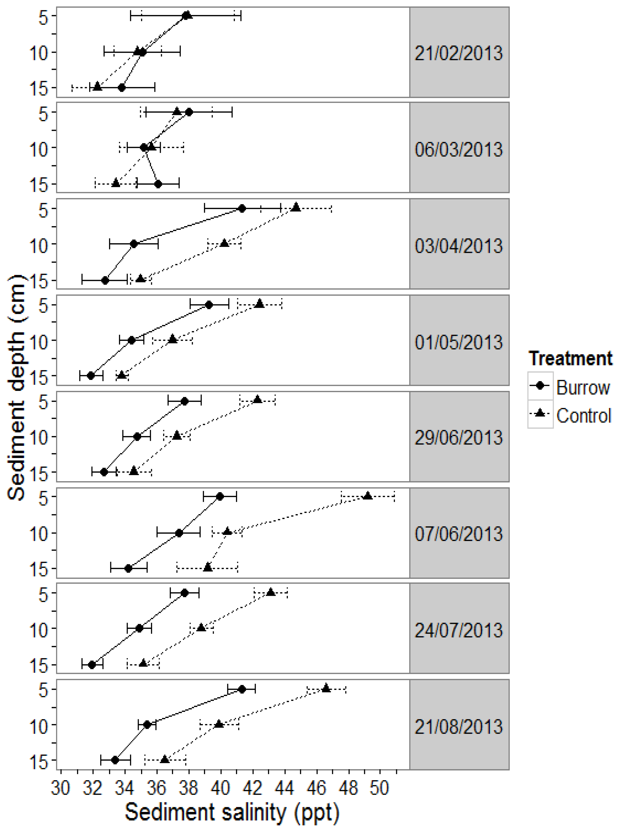
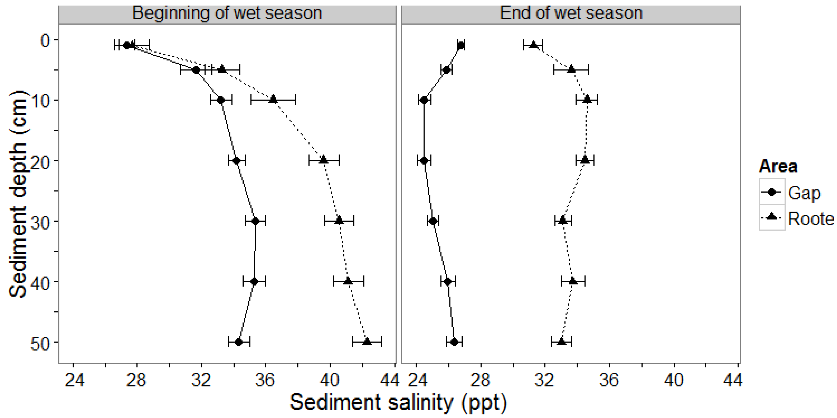
3.1.1. Sediment Salinity

The final model indicates that the pattern of sediment salinity over time in the plant containers differed between the two treatments (with or without artificial burrows). Sediment salinity in both treatments increased. However, in the plant containers without artificial burrows, salinity had a higher increase over time (e.g., from 34 to 40 ppt at 10 cm sediment depth) compared with values for the burrow treatment, which had lower salinity values from the 3rd sampling onwards (e.g., values varied between 34 and 35 ppt at 10 cm sediment depth, Figure 3). A stepwise backwards model selection was applied using a likelihood ratio test including at the beginning sediment depth, treatment and time and their interactions. The interaction term between treatment and time was significant (L. Ratio = 20.9, df = 1, p-value < 0.001, Appendix A1) indicating that the salinity in the control treatment increased more over time than the burrow treatment. Also the interaction term treatment and sediment depth was significant (L. Ratio = 5.1, df = 1, p-value = 0.02, Appendix A1). Thus, mostly due to the differences in treatments over time, the depth-salinity curves differ at each sampling point, e.g., are shallower for the control. In addition, the model with the interaction term between sediment depth and time was significant (L. Ratio = 6.1, df = 1, p-value = 0.01, Appendix A1) resulting in different depth-salinity curves for each sampling date (Figure 3).
Figure 3. Mean sediment salinity (n = 9 for each treatment) inside the plant containers for three sediment depths (5, 10, and 15 cm) from the first sampling (21 February 2013) to the last sampling (21 August 2013). Treatments are indicated by different point and line types. Error bars represent the standard error (SE).
Jmse 03 00539 g003

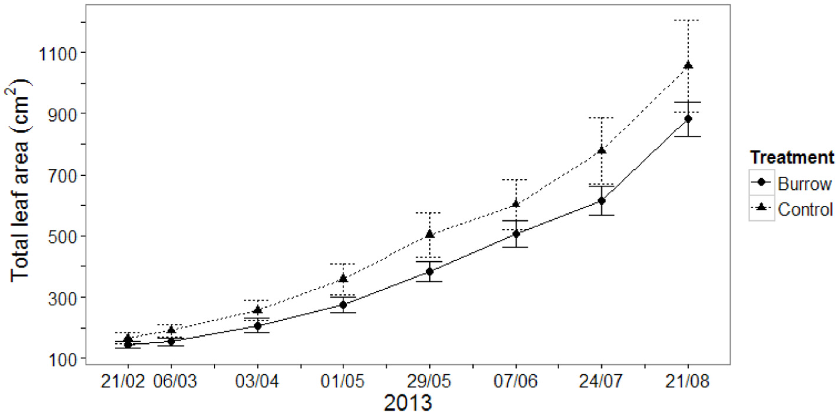
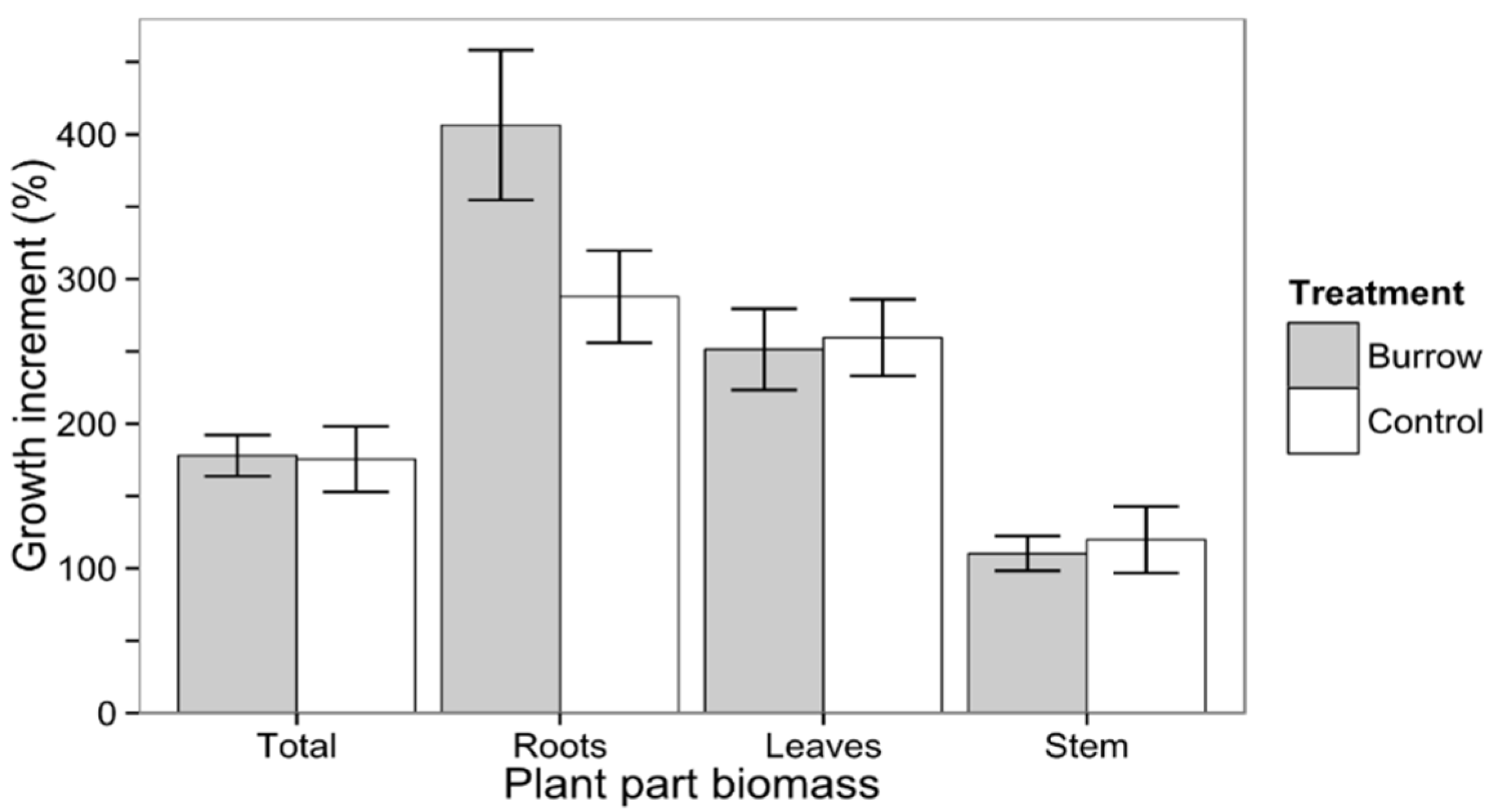
3.1.2. Seedling Growth

The growth increment for the total shoot length of seedlings was similar for both treatments (t-value = 0.5, df = 15, p-value = 0.6, 150.6 ± 12.1%, n = 18).
Log transformed total leaf area increased over time, but did not differ between plant containers with or without artificial crab burrows (Figure 4 showing untransformed data) as indicated by the LME model selection. To select the final model for the log transformed total leaf area data, a model with the interaction term between treatment and time and a model without the interaction term were compared. The interaction term was not significant (L. Ratio = 0.9, df = 1, p-value = 0.4, Appendix A2). Further, the main term treatment was not significant (L. Ratio = 0.9, df = 1, p-value = 0.3, Appendix A2). Only the main term time was significantly term (L. Ratio = 395.2, df = 1, p-value < 0.001, Appendix A2).
The leaf area of the experimental seedlings at each sampling date was calculated with the following regression equation considering the product of leaf length and width:
Leaf area = ((leaf length × leaf width) − 0.3)/1.3, (R2 = 0.95, n = 957)
To estimate the initial dry biomass data for roots, stem/branches and leaves of the experimental seedlings, the regression parameters from Table 1a were used. Growth increments of roots, stem/branches and leaves did not differ significantly between treatments (Table 1b, Figure 5).
Figure 4. Mean total leaf area (cm2, n = 9 for each treatment) from the first sampling (21 February 2013) to the last sampling (21 August 2013). Treatments are indicated by different point and line types. Error bars represent the standard error (SE).
Jmse 03 00539 g004
Figure 5. Mean increment in biomass (%, n = 9 for each treatment) of all plant parts (total) and each single plant part (roots, leaves and stem) between the first sampling (21 February 2013) and the last sampling (21 August 2013). Error bars represent the standard error (SE).
Jmse 03 00539 g005
The model for the ratio between above- and belowground biomass with the interaction between treatment and time was not significant (L. Ratio = 3.7, df = 1, p-value = 0.054, Appendix A3). The main term treatment was also not significant (L. Ratio = 0.0002, df = 1, p-value = 1, Appendix A3). However, a model with the main term time was significant (L. Ratio = 27.4, df = 1, p-value < 0.001, Appendix A3) indicating that the ratio between above- and belowground biomass decreased over time.
Table 1. (a) Regression parameters for dry biomass (DB in g) of each plant part (roots, stem/branches, leaves) against total leaf area (TLA) of each plant listed with the corresponding R2 value and the sample size (n). The regression parameters were used to calculate the DB of each plant part for the first sampling referring to its TLA; (b) Results of t-tests (t-value, df-Degree of freedom and p-value) for the growth increment of each plant part between treatments (burrow, control).
Plant Part Analyses
(a)Regression ParameterR2n
Roots DB = −0.51 + TLA × 0.010.9148
Stem/branches DB = 3.86 + TLA × 0.020.8848
* Leaves DB = 0 + TLA × 0.020.9948
(b)Plant Partt-ValueDfp-Value
roots1.9130.07
stem/branches−0.4120.72
leaves−0.2160.84
* Original regression resulted in negative DB values for the first sampling. Therefore, the regression line was set to cross through the origin.
Figure 6. Mean sediment salinity (n = 21 for each area type) plotted against sediment depth (1, 5, 10, 20, 30, 40 and 50 cm) in gap and rooted areas for the beginning and end of the wet season. Error bars represent the standard error (SE).
Jmse 03 00539 g006

3.2. Field Experiment

The LME model results suggest that area type (rooted and gap areas), sediment depth and season were factors influencing sediment salinity. This can be inferred from the fact that the model with a three-way interaction term was the best model (L. Ratio = 32.1, df = 1, p-value < 0.001, Appendix A4). The interaction resulted in different shapes of the depth-salinity curve for gap and rooted areas and for different sampling dates (Figure 6). At the beginning and at the end of the wet season, sediment salinity was generally higher in rooted areas compared with gap areas. However, at the beginning of the wet season, sediment salinities of rooted and gap areas were similar for 1 and 5 cm sediment depths. Sediment salinities increased with sediment depths and from 10 cm depth onwards they were higher in rooted areas (Figure 6).
Crab burrow density was significantly higher in rooted areas for the beginning of wet season with 7.6 ± 0.5 burrows m−2 (n = 21) and the end of wet season with 8.2 ± 0.4 burrows m−2 (n = 21) than in gaps for the beginning of wet season with 2.4 ± 0.4 burrows m−2 (n = 21) and the end of wet season with 3.0 ± 0.7 burrows m−2 (n = 21). The interaction between area type and season was not significant (L. Ratio = 0.001, df = 1, p-value = 1, Appendix A5). Additionally, including the main term season into the model, did not yield a better result (L. Ratio = 1.8, df = 1, p-value = 0.2, Appendix A5). However, taking into account the main term area type resulted in a significantly better model (L. Ratio = 75.4, df = 1, p-value < 0.001, Appendix A5).

4. Discussion

4.1. Microcosm Experiment

Macro-pores modeled after crab burrows with one opening facilitated the release of salt accumulating around mangrove tree roots from the sediment under controlled microcosm conditions. Sediment salinity increased over time under both treatments at all three depths. However, the increase was significantly stronger in the control than in the burrow treatment. Sediment salinity decreased with increasing sediment depth, most likely because salt accumulated not exclusively around the roots of the mangrove seedlings, but also near the sediment surface due to evaporation during exposition to air.
Possible mechanisms leading to the desalting of sediment are tidal pumping and flushing. First, tidal pumping is considered. Xin et al. [23] simulated the influence of simple burrows of Uca arcuata on the pore and groundwater flow through sediments of salt marshes: During flood tide, ground water dwelled up into burrows and during ebb tide water from higher sediment layers drained through burrows. The authors suggested that these processes improved the pore and groundwater flow and increased the solute exchange between the sediment and tidal water (e.g., diffusion of salt accumulated around roots to burrow water). Results of our microcosm experiment confirm the simulations of Xin et al. [23] by showing that simple burrows indeed reduce the concentrations of solutes in the sediment. In U-shaped, multiple-looped and complex burrows the topographical slope of the sediment can create a pressure difference between the two or more openings. Thus, when the incoming tide arrives and enters first at one opening, a water flow can evolve between the former and the remaining openings [10,24,25]. No such flux is expected for simple burrows like those of U. cordatus; however, sudden influx of water spilling over the edge of the burrow openings at high tide and turbulence caused by surface flow passing over already flooded burrow openings will certainly enhance mixing with water accumulated in the burrow. Thus, a combination of macro-pore enhanced tidal pumping, flushing and increased contact between the sediment surface and water most likely favored release of solutes from sediment in the microcosm experiment. Our experiment and the available simulation models provide a starting point for future studies of the role of simple burrows in the field. Some factors to consider in future studies to identify the importance of these mechanisms under natural conditions are (1) the structure and depth of a burrow, which may influence the amount and velocity of water flow [10,24,25], (2) the difference in water densities between surface and burrow water, which influences the mixing efficiency between those two water bodies [11] and (3) active irrigation by inhabitants of burrows which may enhance mixing of tidal with burrow water [10]. Another aspect to consider is whether burrow entrances are closed or open during flood tides. In the microcosm experiment the artificial burrows were always open, which is not always the case under natural conditions as for example U. cordatus can close its burrows [50].
In this microcosm experiment, seedling growth did not differ between treatments, although sediment salinities differed. Leaf area growth appeared to be higher for control plants (Figure 4), but variance between seedlings was high and statistical results did not confirm this trend. Experiments testing the growth of Rhizophora seedlings under different salinity conditions have shown that growth is generally enhanced at lower salinities [51,52,53,54] and seems to be at its optimum at salinities of 8 and 18 for different Rhizophora species [51,52,53]. Krauss & Allen [53] studied the growth of R. mangle seedlings in salinities of 2, 10, and 32 ppt. Although the relative growth rate (measured by total biomass) was significantly higher at a salinity of 10 ppt, other growth parameters (leaf area, seedling height) did not significantly differ between salinity levels. They concluded that, within the range tested in their experiment, salinity is of minor importance for the growth of R. mangle [53]. Experiments testing seedling growth in salinities of up to 60 ppt showed that seedlings can survive and grow in sediments with such high salinities. However, for salinities higher than the optimum growth range, growth rates significantly decreased and above a salinity of 45 ppt even leaf necrosis (“burn marks”) appeared [51,52]. Salinities in our experiment ranged from 31 to 46 ppt, thus, according to the studies mentioned above, seedlings did not experience optimum growth conditions. However, necrosis of leaves did not occur during the experiment, indicating that seedlings may have sustained limited growth, but did not suffer severe damage.
Salinity differences between treatments were small when compared with the range in which seedlings can potentially grow. For example at the last sampling the salinity difference between treatments was approximately 4 ppt in 10 cm sediment depth (Figure 3). Therefore, it is assumed that these differences between treatments did not influence the seedling growth considerably, because the plants can cope with much higher salinity differences. Moreover, above mentioned growth experiments found differences in growth due to different salinities within a time period of 3–9 months [52,53,54]. Thus, it seems unlikely that the time span of the experiment of this study (6 months) was too short for growth differences to evolve, indicating again that the salinity difference may not have been pronounced enough to be relevant for plant growth.
Although the seedlings experienced similar water salinities and light intensities during the experiment, the increment in total shoot length, dry biomass of different plant parts and total leaf area strongly differed between individual seedlings within treatments. This may be due to genetic differences or internal reserves of the seedlings masking growth differences between treatments [55]. Since the size of the propagule from which the seedling developed could not be determined until the end of the experiment, when plants were dug out, it was unclear how much internal reserves each seedling had at the onset of the experiment.
Another parameter to evaluate seedling growth is the ratio between above- and belowground dry biomass. Mangrove tree seedlings may react to elevated salinities by increasing their root versus above-ground biomass (e.g., [56,57]). No such effect was detected in our microcosm experiment. Again, salinity differences between treatments might have been insufficiently large to trigger the expected response. At any rate, the belowground/aboveground ratio may be subject to shifts dependent on developmental stage [58] which could not be analyzed in our experimental setup.

4.2. Mangrove Sediment Salinity

In the Caeté estuary, densely rooted sediment with distinctly elevated sediment salinities coincided with high U. cordatus burrow densities, whereas the salinity was lower in sediment with no or few roots and low burrow densities. Similarly, Smith III [59] measured higher salinities in rooted sediment (57.5 ppt) compared with sparsely rooted forest gaps (55.2 ppt) in a high intertidal North Australian mangrove forest, but the author does not provide corresponding data on crab burrow density. At first glance, these results contradicts our initial hypothesis that burrows facilitate the removal of accumulated salt. However, salt accumulation by mangrove trees may mask the desalting effect of burrows, because a much larger quantity of salt may be accumulated in rooted sediment areas than can be removed by burrows resulting in a net increase in sediment salinity. In an Australian Rhizophora forest, burrow water conductivity (as proxy for salinity) of a Sesarma sp. burrow was monitored at 70 cm depth over 15 days [60]. The burrows of these crabs are multiple-looped and/or complex with more than one opening [12]. During spring high tides when tidal flushing occurred, burrow water conductivity was similar to tidal water conductivity and during periods of rainfall, burrow water conductivity decreased. These results clearly show the influence of rainfall and tidal flushing on the water accumulated within the burrow. However, during days without tidal flushing or rainfall, conductivity increased monotonically over time, indicating a diffusion process of salt from the sediment into the burrow water [60]. The results by Stieglitz et al. [60] and from our microcosm experiment strongly indicate that burrows facilitate desalting of the sediment and that results in the field study are masked by a much higher salt accumulation by tree roots or desalting by precipitation. Additionally, U. cordatus burrows are not always open [50], thus, the desalting process may be stopped or less efficient when burrows are closed.
Sediment salinity generally decreased from the first sampling at the beginning of the wet season until the second sampling at the end of the wet season for both area types, indicating that precipitation has an important role in regulating sediment salinities, as also seen in other studies [9,61]. The precipitation-related changes in sediment salinity influence the growth and phenology of R. mangle trees (in the study area: [62,63]).
The shape of the salinity-depth curve from the initial phase of the rainy season indicates that rainwater had already reduced the salt concentration at the surface, whereas salt accumulated in deeper sediment layers during the previous dry season was still present. With the continuing rainfalls, salt concentrations had been reduced in the deeper layers when we sampled again at the end of the wet season. This reduction of solute concentrations was more pronounced in the areas without stilt roots, where salt accumulation by the trees should be negligible. However, surface salinity in the areas with stilt roots was even slightly higher than at the beginning of the rainy season, indicating that the diminishing rainfall was no longer able to compensate the salt accumulation by evaporation at the sediment surface.
To study the influence of single factors on the desalting of sediment under natural conditions is difficult, due to many confounding factors such as sediment salinity, precipitation, evaporation, burrow density, root biomass and sediment characteristics (e.g., salt lenses or grain size). A possible method to indirectly estimate the influence of crab burrows on the salt release may be the exclusion of crabs from experimental plots and thereby a reduction of burrows.

5. Conclusions

This study is the first to show that artificial crab burrows with one opening facilitated salt release from rooted sediment in a microcosm experiment. However, the amount of salt released was not high enough to increase seedling growth. In addition to the microcosm results, field data from a R. mangle mangrove forest showed that high sediment salinity was associated with the presence of stilt roots. These areas are also the preferred habitat of U. cordatus; the high burrow density of this crab species in well-rooted areas does, nevertheless, not result in a net decrease of sediment salinity. The desalting effect of burrows appears to be masked by the salt accumulation of tree roots or by frequent salt wash outs during heavy rainfalls in the wet season. Future research should investigate the desalting by simple burrows also in the dry season to reveal whether the crabs’ functional role regarding this important ecosystem process differs seasonally. The results of this study further show how experimental and observational studies can complement each other. Although in the field study the desalting effect was likely masked by other confounding parameter, the microcosm experiment clearly shows that artificial burrows with one opening facilitate desalting. Merely a field study would not be able to identify this process by itself, thus, investigating single processes within an experimental setting may help understand ecosystem processes better.

Acknowledgments

We thank the Instituto do Estudos Costeiros (IECOS) of the Federal University of Pará (UFPA) in Brazil providing laboratory and greenhouse facilities, the Instituto Chico Mendes de Conservação da Biodiversidade (ICMBIO) and the Stakeholder Council of the Reserva Extrativista (RESEX) Caeté-Taperaçu for their support. Further we thank Marlana Cristina Queiroz da Silva and Amanda Reis da Silva, for their help in the field and with the seedlings. We also thank the anonymous reviewers for their help. Travel grants for Ulf Mehlig were provided by the Coastal Research Network for Environmental Changes. Karen Diele received funding from the MASTS pooling initiative (The Marine Alliance for Science and Technology for Scotland) and its support is gratefully acknowledged. MASTS is funded by the Scottish Funding Council (grant reference HR09011) and contributing institutions.

Author Contributions

Nathalie Pülmanns, Inga Nordhaus, Karen Diele and Ulf Mehlig conceived and designed the experiments; Nathalie Pülmanns performed the experiments; Nathalie Pülmanns analyzed the data; Ulf Mehlig contributed reagents/materials/analysis tools; Nathalie Pülmanns, Inga Nordhaus, Karen Diele and Ulf Mehlig wrote the paper.

Conflicts of Interest

The authors declare no conflict of interest.

Appendix

Appendix A1

The final optimal model was selected after a stepwise backwards model selection using the likelihood ratio test.
Sediment salinityip ~ α + Sediment depthip + Treatmentip + Timeip + Sediment depthip × Treatmentip + Sediment depthip × Timeip + Treatmentip × Timeip + ap + εip, εip ~ N(0,σ2)
Sediment salinityip is the sediment salinity of observation i for plant p, where p runs from 1 to 18, and i is the observation for each plant that ranges from 1 to 8 (the number of samplings over time). The final model above means that sediment salinity is modeled as a function of sediment depth, treatment, time and all their two way interaction terms. Treatment is a categorical covariate and sediment depth and time a continuous. The term ap is the random effect representing the between-plant variation and is significant (L. Ratio = 51.8, df = 1, p-value < 0.001). The unexplained variance ε is assumed to be normally distributed with mean 0 and variance σ2. The intercept of the model is represented with α.

Appendix A2

The final optimal model was selected after a stepwise backwards model selection using the likelihood ratio test.
log(total leaf area)ip ~ α + Timeip + ap + εip, εip ~ N(0,σ2)
Log transformed total leaf areaip is the observation i for plant p, where p runs from 1 to 18, and i is the observation for each plant that ranges from 1 to 8 (the number of samplings over time). The final model above means that log transformed total leaf areas is modeled as a function of time. Time is a continuous covariate. The term ap is the random effect representing the between-plant variation and is significant (L. Ratio = 211.7, df = 1, p-value < 0.001). The unexplained variance ɛ is assumed to be normally distributed with mean 0 and variance σ2. The intercept of the model is represented with α.

Appendix A3

The final optimal model was selected after a stepwise backwards model selection with the likelihood ratio test.
Above: below ground ratioip ~ α + Timeip + ap + εip, εip ~ N(0,σ2)
Above to below ground ratioip is the observation i for plant p, where p runs from 1 to 18, and i is the observation for each plant that ranges from 1 to 2 (first and last sampling). The final model above means that above to below ground ratio is modeled as a function of time. Time is a continuous covariate. The term ap is the random effect representing the between-plant variation and is significant (L. Ratio = 9.5, df = 1, p-value = 0.002). The unexplained variance ɛ is assumed to be normally distributed with mean 0 and variance σ2. The intercept of the model is represented with α.

Appendix A4

The final optimal model was selected after a stepwise backwards model selection using the likelihood ratio test.
Sediment salinityics ~ α + Sediment depthics + Area typeics + Seasonics + Sediment depthics × Area typeics + Sediment depthics × Seasonics + Area typeics × Seasonics + Sediment depthics × Area typeics × Seasonics+ as + ac/s + εics, εics ~ N(0,σd2)
Sediment salinityics is the observation i for each sediment core c at each sampling site s, where c runs from 1 to 3, s from 1 to 7 and i is the observation for each core at the different sites that ranges from 1 to 2 (the number of samplings). The final model above means that sediment salinity is modeled as a function of sediment depth, area type, season and all their two and three way interactions. Season and area type are categorical covariates. The terms as and ac/s are random effects representing the between-sampling site and between-core variation and are significant (L. Ratio = 11.7, df = 1, p-value < 0.001, nested term: L. Ratio = 64.4, df = 1, p-value < 0.001). The unexplained variance ɛics is assumed to be normally distributed with mean 0 and variance σ2d where d takes 7 different values according to each sediment depth level. The intercept of the model is represented with α.

Appendix A5

The final optimal model was selected after a stepwise backwards model selection using the likelihood ratio test:
Burrow densityis ~ α + Area typeis + Seasonis + Area typeis × Seasonis + as + εis, εis ~ N(0,σ2)
Burrow densityis is the observation i for each sampling site s, where s runs from 1 to 7 and i is the observation at the different sites that ranges from 1 to 2 (the number of samplings). The final model above means that burrow density is modeled as a function of area type, season and their interaction. Season and area type are categorical covariates. The term as is a random effect representing the between-sampling site variation and is significant (L. Ratio = 7.1, df = 1, p-value = 0.008). The unexplained variance ɛis is assumed to be normally distributed with mean 0 and variance σ2.

References

  1. Ball, M.C. Ecophysiology of mangroves. Trees 1988, 2, 129–142. [Google Scholar] [CrossRef]
  2. Gill, A.M.; Tomlinson, P.B. Studies on the growth of red mangrove (Rhizophora mangle L.) 4. The adult root system. Biotropica 1977, 9, 145–155. [Google Scholar] [CrossRef]
  3. Passioura, J.B.; Ball, M.C.; Knight, J.H. Mangroves may salinize the soil and in so doing limit their transpiration rate. Funct. Ecol. 1992, 6, 476–481. [Google Scholar] [CrossRef]
  4. Alongi, D.M.; Tirendi, F.; Dixon, P.; Trott, L.A.; Brunskill, G.J. Mineralization of organic matter in intertidal sediments of a tropical semi-enclosed delta. Estuar. Coast. Shelf Sci. 1999, 48, 451–467. [Google Scholar] [CrossRef]
  5. Holmer, M.; Andersen, F.Ø.; Holmboe, N.; Kristensen, E.; Thongtham, N. Transformation and exchange processes in the Bangrong mangrove forest-seagrass bed system, Thailand. Seasonal and spatial variations in benthic metabolism and sulfur biogeochemistry. Aquat. Microb. Ecol. 1999, 20, 203–212. [Google Scholar] [CrossRef]
  6. Schwendenmann, L.; Riecke, R.; Lara, R.J. Solute dynamics in a North Brazilian mangrove: The influence of sediment permeability and freshwater input. Wetl. Ecol. Manag. 2006, 14, 463–475. [Google Scholar] [CrossRef]
  7. Hollins, S.E.; Ridd, P.V.; Read, W.W. Measurement of the diffusion coefficient for salt in salt flat and mangrove soils. Wetl. Ecol. Manag. 2000, 8, 257–262. [Google Scholar] [CrossRef]
  8. Stieglitz, T.C.; Clark, J.F.; Hancock, G.J. The mangrove pump: The tidal flushing of animal burrows in a tropical mangrove forest determined from radionuclide budgets. Geochim. Cosmochim. Acta 2013, 102, 12–22. [Google Scholar] [CrossRef] [Green Version]
  9. Wolanski, E.; Gardiner, R. Flushing of salt from mangrove swamps. Mar. Freshw. Res. 1981, 32, 681–683. [Google Scholar] [CrossRef]
  10. Heron, S.F.; Ridd, P.V. The tidal flushing of multiple-loop animal burrows. Estuar. Coast. Shelf Sci. 2008, 78, 135–144. [Google Scholar] [CrossRef]
  11. Heron, S.F.; Ridd, P.V. The effect of water density variations on the tidal flushing of animal burrows. Estuar. Coast. Shelf Sci. 2003, 58, 137–145. [Google Scholar] [CrossRef]
  12. Stieglitz, T.C.; Ridd, P.V.; Müller, P. Passive irrigation and functional morphology of crustacean burrows in a tropical mangrove swamp. Hydrobiologia 2000, 421, 69–76. [Google Scholar] [CrossRef]
  13. Colbert, S.L.; Berelson, W.M.; Hammond, D.E. Radon-222 budget in Catalina Harbor, California: 2. Flow dynamics and residence time in a tidal beach. Limnol. Oceanogr. 2008, 53, 659–665. [Google Scholar] [CrossRef]
  14. Li, X.; Hu, B.X.; Burnett, W.C.; Santos, I.R.; Chanton, J.P. Submarine ground water discharge driven by tidal pumping in a heterogeneous aquifer. Ground Water 2009, 47, 558–568. [Google Scholar] [CrossRef] [PubMed]
  15. Susilo, A.; Ridd, P.V.; Thomas, S. Comparison between tidally driven groundwater flow and flushing of animal burrows in tropical mangrove swamps. Wetl. Ecol. Manag. 2005, 13, 377–388. [Google Scholar] [CrossRef]
  16. Adame, M.F.; Virdis, B.; Lovelock, C.E. Effect of geomorphological setting and rainfall on nutrient exchange in mangroves during tidal inundation. Mar. Freshw. Res. 2010, 61, 1197–1206. [Google Scholar] [CrossRef]
  17. Akamatsu, Y.; Ikeda, S.; Toda, Y. Transport of nutrients and organic matter in a mangrove swamp. Estuar. Coast. Shelf Sci. 2009, 82, 233–242. [Google Scholar] [CrossRef]
  18. Bouillon, S.; Middelburg, J.J.; Dehairs, F.; Borges, A.V.; Abril, G.; Flindt, M.R.; Ulomi, S.; Kristensen, E. Importance of intertidal sediment processes and porewater exchange on the water column biogeochemistry in a pristine mangrove creek (Ras Dege, Tanzania). Biogeosciences 2007, 4, 311–322. [Google Scholar] [CrossRef]
  19. Gleeson, J.; Santos, I.R.; Maher, D.T.; Golsby-Smith, L. Groundwater-surface water exchange in a mangrove tidal creek: Evidence from natural geochemical tracers and implications for nutrient budgets. Mar. Chem. 2013, 156, 27–37. [Google Scholar] [CrossRef]
  20. Lara, R.J.; Dittmar, T. Nutrient dynamics in a mangrove creek (North Brazil) during the dry season. Mangroves salt marshes 1999, 3, 185–195. [Google Scholar] [CrossRef]
  21. Maher, D.T.; Santos, I.R.; Golsby-Smith, L.; Gleeson, J.; Eyre, B.D. Groundwater-derived dissolved inorganic and organic carbon exports from a mangrove tidal creek: The missing mangrove carbon sink? Limnol. Ocean. 2013, 58, 475–488. [Google Scholar]
  22. Mazda, Y.; Ikeda, Y. Behavior of the groundwater in a riverine-type mangrove forest. Wetl. Ecol. Manag. 2006, 14, 477–488. [Google Scholar] [CrossRef]
  23. Xin, P.; Jin, G.; Li, L.; Barry, D.A. Effects of crab burrows on pore water flows in salt marshes. Adv. Water Resour. 2009, 32, 439–449. [Google Scholar] [CrossRef]
  24. Heron, S.F.; Ridd, P.V. The use of computational fluid dynamics in predicting the tidal flushing of animal burrows. Estuar. Coast. Shelf Sci. 2001, 52, 411–421. [Google Scholar] [CrossRef]
  25. Ridd, P.V. Flow through animal burrows in mangrove creeks. Estuar. Coast. Shelf Sci. 1996, 43, 617–625. [Google Scholar] [CrossRef]
  26. Cannicci, S.; Burrows, D.; Fratini, S.; Smith, T.J., III; Offenberg, J.; Dahdouh-Guebas, F. Faunal impact on vegetation structure and ecosystem function in mangrove forests: A review. Aquat. Bot. 2008, 89, 186–200. [Google Scholar] [CrossRef]
  27. Katz, L.C. Effects of burrowing by the fiddler crab, Uca pugnax (Smith). Estuar. Coast. Mar. Sci. 1980, 11, 233–237. [Google Scholar] [CrossRef]
  28. Kristensen, E. Organic matter diagenesis at the oxic/anoxic interface in coastal marine sediments, with emphasis on the role of burrowing animals. Hydrobiologia 2000, 426, 1–24. [Google Scholar] [CrossRef]
  29. Qureshi, N.A.; Saher, N.U. Burrow morphology of three species of fiddler crab (Uca) along the coast of Pakistan. Belg. J. Zool. 2012, 142, 114–126. [Google Scholar]
  30. Thongtham, N.; Kristensen, E. Physical and chemical characteristics of mangrove crab (Neoepisesarma versicolor) burrows in the Bangrong mangrove forest, Phuket, Thailand; with emphasis on behavioural response to. Vie Milieu 2003, 53, 141–151. [Google Scholar]
  31. Schories, D.; Barletta-Bergan, A.; Barletta, M.; Krumme, U.; Mehlig, U.; Rademaker, V. The keystone role of leaf-removing crabs in mangrove forests of North Brazil. Wetl. Ecol. Manag. 2003, 11, 243–255. [Google Scholar] [CrossRef]
  32. Diele, K.; Koch, V.; Saint-Paul, U. Population structure, catch composition and CPUE of the artisanally harvested mangrove crab Ucides cordatus (Ocypodidae) in the Caeté estuary, North Brazil: Indications for overfishing? Aquat. Living Resour. 2005, 18, 169–178. [Google Scholar] [CrossRef]
  33. Tavares, M. True Crabs. In The Living Marine Resources of the Western Central Atlantic; Carpenter, K.E., Ed.; Food and Agriculture Organization (FAO): Rome, Italy, 2003; pp. 327–352. [Google Scholar]
  34. Piou, C.; Berger, U.; Feller, I.C. Spatial structure of a leaf-removing crab population in a mangrove of North-Brazil. Wetl. Ecol. Manag. 2009, 17, 93–106. [Google Scholar] [CrossRef]
  35. Tamooh, F.; Huxham, M.; Karachi, M.; Mencuccini, M.; Kairo, J.G.; Kirui, B. Below-ground root yield and distribution in natural and replanted mangrove forests at Gazi bay, Kenya. For. Ecol. Manag. 2008, 256, 1290–1297. [Google Scholar] [CrossRef]
  36. Araújo, J.M.C., Jr.; Otero, X.L.; Marques, A.G.B.; Nóbrega, G.N.; Silva, J.R.F.; Ferreira, T.O. Selective geochemistry of iron in mangrove soils in a semiarid tropical climate: Effects of the burrowing activity of the crabs Ucides cordatus and Uca maracoani. Geo-Mar. Lett. 2012, 32, 289–300. [Google Scholar] [CrossRef]
  37. Bouillon, S.; Koedam, N.; Raman, A.V.; Dehairs, F. Primary producers sustaining macro-invertebrate communities in intertidal mangrove forests. Oecologia 2002, 130, 441–448. [Google Scholar] [Green Version]
  38. Dye, A.H.; Lasiak, T.A. Microbenthos, meiobenthos and fiddler crabs: Trophic interactions in a tropical mangrove sediment. Mar. Ecol. Prog. Ser. 1986, 32, 259–264. [Google Scholar] [CrossRef]
  39. France, R. Estimating the assimilation of mangrove detritus by fiddler crabs in Laguna Joyuda, Puerto Rico, using dual stable isotopes. J. Trop. Ecol. 1998, 14, 413–425. [Google Scholar] [CrossRef]
  40. Miller, D.C. The feeding mechanism of fiddler crabs, with ecological considerations of feeding adaptations. Zoologica 1961, 46, 89–101. [Google Scholar]
  41. Mehlig, U.; Menezes, M.P.M.; Reise, A.; Schories, D.; Medina, E. Mangrove Vegetation of the Caeté Estuary. In Mangrove Dynamics and Management in North Brazil; Saint-Paul, U., Schneider, H., Eds.; Ecological Studies; Springer: Berlin, Germany, 2010; Volume 211, pp. 71–107. [Google Scholar]
  42. INMET. Available online: http://www.inmet.gov.br (accessed on 15 January 2013).
  43. Brabo, L.B. Medidas de Trocas Gasosas de Plantas de Manguezal sob Diferentes Condições de Salinidade e Inundação em Estufa e Campo (Bragança-PA-Brasil); Universidade federal do Pará, Campus universitário de Bragança: Belem, Bragança, Brazil, 2004. [Google Scholar]
  44. Steubing, L.; Fangmeier, A. Pflanzenökologisches Praktikum: Gelände- und Laborpraktikum der terrestrischen Pflanzenökologie; Ulmer: Stuttgart, Germany, 1992. [Google Scholar]
  45. Pinheiro, J.C.; Bates, D.M.; DebRoy, S.; Sarkar, D. nlme: Linear and Nonlinear Mixed Effects Models. In R Package Version; R Foundation for Statistical Computing: Vienna, Austria, 2012; pp. 1–102. [Google Scholar]
  46. Wickham, H. Ggplot2: Elegant Graphics for Data Analysis; Springer Science & Business Media: Berlin, Germany, 2009. [Google Scholar]
  47. Zuur, A.F.; Ieno, E.N.; Elphick, C.S. A protocol for data exploration to avoid common statistical problems. Methods Ecol. Evol. 2010, 1, 3–14. [Google Scholar] [CrossRef]
  48. Zuur, A.F.; Ieno, E.N.; Walker, N.; Saveliev, A.A.; Smith, G.M. Mixed Effects Models and Extensions in Ecology with R; Springer: New York, NY, USA, 2009. [Google Scholar]
  49. Zuur, A.F.; Ieno, E.N.; Smith, G.M. Analyzing Ecological Data; Springer: New York, NY, USA, 2007. [Google Scholar]
  50. Nordhaus, I.; Diele, K.; Wolff, M. Activity patterns, feeding and burrowing behaviour of the crab Ucides cordatus (Ucididae) in a high intertidal mangrove forest in North Brazil. J. Exp. Mar. Bio. Ecol. 2009, 374, 104–112. [Google Scholar] [CrossRef]
  51. Biber, P.D. Measuring the effects of salinity stress in the red mangrove, Rhizophora mangle L. Afr. J. Agric. Res. 2006, 1, 1–4. [Google Scholar]
  52. Hoppe-Speer, S.C.L.; Adams, J.B.; Rajkaran, A.; Bailey, D. The response of the red mangrove Rhizophora mucronata Lam. to salinity and inundation in South Africa. Aquat. Bot. 2011, 95, 71–76. [Google Scholar] [CrossRef]
  53. Krauss, K.W.; Allen, J.A. Influences of salinity and shade on seedling photosynthesis and growth of two mangrove species, Rhizophora mangle and Bruguiera sexangula, introduced to Hawaii. Aquat. Bot. 2003, 77, 311–324. [Google Scholar] [CrossRef]
  54. Smith, S.M.; Snedaker, S.C. Salinity responses in two populations of viviparous Rhizophora mangle L. seedlings. Biotropica 1995, 27, 435–440. [Google Scholar] [CrossRef]
  55. Lin, G.; Sternberg, L.S.L. Effect of growth form, salinity, nutrient and sulfide on photosynthesis, carbon isotope discrimination and growth of red mangrove (Rhizophora mangle L.). Funct. Plant. Biol. 1992, 19, 509–517. [Google Scholar]
  56. Ball, M.C.; Cochrane, M.J.; Rawson, H.M. Growth and water use of the mangroves Rhizophora apiculata and R. stylosa in response to salinity and humidity under ambient and elevated concentrations of atmospheric CO2. Plant Cell Environ. 1997, 20, 1158–1166. [Google Scholar] [CrossRef]
  57. López-Hoffman, L.; Anten, N.P.R.; Martínez-Ramos, M.; Ackerly, D.D. Salinity and light interactively affect neotropical mangrove seedlings at the leaf and whole plant levels. Oecologia 2007, 150, 545–556. [Google Scholar] [CrossRef] [PubMed]
  58. Komiyama, A.; Ong, J.E.; Poungparn, S. Allometry, biomass, and productivity of mangrove forests: A review. Aquat. Bot. 2008, 89, 128–137. [Google Scholar] [CrossRef]
  59. Smith, T.J., III. Effects of seed predators and light level on the distribution of Avicennia marina (Forsk.) Vierh in tropical, tidal forests. Estuar. Coast. Shelf Sci. 1987, 25, 43–51. [Google Scholar] [CrossRef]
  60. Stieglitz, T.C.; Ridd, P.V.; Hollins, S.E. A small sensor for detecting animal burrows and monitoring burrow water conductivity. Wetl. Ecol. Manag. 2000, 8, 1–7. [Google Scholar] [CrossRef]
  61. Marchand, C.; Baltzer, F.; Lallier-Vergès, E.; Albéric, P. Pore-water chemistry in mangrove sediments: Relationship with species composition and developmental stages (French Guiana). Mar. Geol. 2004, 208, 361–381. [Google Scholar] [CrossRef] [Green Version]
  62. Mehlig, U. Phenology of the red mangrove, Rhizophora mangle L., in the Caeté Estuary, Pará, equatorial Brazil. Aquat. Bot. 2006, 84, 158–164. [Google Scholar] [CrossRef]
  63. Menezes, M.; Berger, U.; Worbes, M. Annual growth rings and long-term growth patterns of mangrove trees from the Bragança peninsula, North Brazil. Wetl. Ecol. Manag. 2003, 11, 233–242. [Google Scholar] [CrossRef]

