Article

Gauge-Invariant Formulation of Time-Dependent Configuration Interaction Singles Method

by
Takeshi Sato
1,2,
Takuma Teramura
1 and
Kenichi L. Ishikawa
1,2,*
1
Department of Nuclear Engineering and Management, School of Engineering, The University of Tokyo, 7-3-1 Hongo, Bunkyo-ku, Tokyo 113-8656, Japan
2
Photon Science Center, School of Engineering, The University of Tokyo, 7-3-1 Hongo, Bunkyo-ku, Tokyo 113-8656, Japan
*
Author to whom correspondence should be addressed.
Appl. Sci. 2018, 8(3), 433; https://doi.org/10.3390/app8030433
Submission received: 31 January 2018 / Revised: 6 March 2018 / Accepted: 8 March 2018 / Published: 13 March 2018
(This article belongs to the Special Issue Attosecond Science and Technology: Principles and Applications)

Abstract

:
We propose a gauge-invariant formulation of the channel orbital-based time-dependent configuration interaction singles (TDCIS) method [Phys. Rev. A, 74, 043420 (2006)], one of the powerful ab initio methods to investigate electron dynamics in atoms and molecules subject to an external laser field. In the present formulation, we derive the equations of motion (EOMs) in the velocity gauge using gauge-transformed time-dependent, not fixed, orbitals that are equivalent to the conventional EOMs in the length gauge using fixed orbitals. The new velocity-gauge EOMs avoid the use of the length-gauge dipole operator, which diverges at large distance, and allows us to exploit computational advantages of the velocity-gauge treatment over the length-gauge one, e.g., a faster convergence in simulations with intense and long-wavelength lasers, and the feasibility of exterior complex scaling as an absorbing boundary. The reformulated TDCIS method is applied to an exactly solvable model of one-dimensional helium atom in an intense laser field to numerically demonstrate the gauge invariance. We also discuss the consistent method for evaluating the time derivative of an observable, which is relevant, e.g., in simulating high-harmonic generation.

1. Introduction

Time-dependent configuration interaction singles (TDCIS) method is one of the powerful ab initio methods to investigate laser-driven electron dynamics in atoms and molecules [1,2,3,4,5,6,7,8,9,10,11,12,13,14,15,16,17,18,19,20,21,22,23,24]. In the TDCIS method, the time-dependent electronic wavefunction is given by the configuration interaction (CI) expansion,
Ψ ( t ) = Φ C 0 ( t ) + i o c c a v i r Φ i a C i a ( t ) ,
where Φ is the ground-state Hartree-Fock (HF) wavefunction, and Φ i a is a singly-excited configuration-state function (CSF), replacing an occupied HF orbital ϕ i in Φ with a virtual (unoccupied in Φ ) orbital ϕ a , and the electron dynamics is described through the time evolution of the CI coefficients, C 0 and { C i a } . The virtual orbitals { ϕ a } consist, in theory, of an infinite number of bound and continuum orbitals. In practice, one needs to work within a given, finite number of basis functions or numerical grids to represent orbitals; however, the real-space implementation with an appropriate absorbing boundary has been proved to correctly model both bound and continuum states, allowing to describe electron dynamics involving both (single) excitations and ionizations [4]. Compared to more involved ab initio wavefunction-based approaches [25] such as time-dependent multiconfiguration self-consistent-field (TD-MCSCF) methods [26,27,28,29,30,31,32,33], time-dependent R-matrix based approaches [34,35,36], or time-dependent reduced density-matrix approach [37,38], distinct advantages of the TDCIS method include a low computational cost and the conceptual simplicity to analyze simulation results. Furthermore, an effective one-electron theory with coupled channels has been developed [2], which introduces the orbital-like quantity, called channel orbital,
χ i ( r , t ) = a ϕ a ( r ) C i a ( t ) ,
and equivalently rewrites EOMs for CI coefficients with those for channel orbitals { χ i ( r , t ) } with no individual reference to virtual orbitals. This reformulation removes the bottleneck of the CI coefficient-based TDCIS method to compute all (or, at least sufficiently many, including bound and continuum) virtual orbitals prior to the simulation, and thus particularly useful in grid-based simulations.
Despite this advantage, numerical applications of the channel orbital-based TDCIS method has been limited to Ref. [2,14,15] for a one-dimensional Hamiltonian and Ref. [1] for noble gas atoms with a Hartree-Slater potential, as far as we know, and the vast majority of applications to date have adopted the CI coefficient-based approach [3,4,5,6,7,8,9,10,11,12,13,16,17,18,19,20,21,22,23,24] , except for the use of { χ i } as intermediate quantities in evaluating photoelectron spectra [18]. The preference of CI coefficient-based approach might be partially due to the high symmetry of atomic systems, for which the stationary Hartree-Fock operator decouples for different angular momenta [4], making it a relatively feasible task to obtain all virtual orbitals (within a given radial grids or radial basis functions) for the lowest few angular momenta. The channel orbital-based approach would be more suited, on the other hand, to simulations of electron dynamics with intense and/or long-wavelength laser fields, requiring much longer angular momentum expansion [39,40,41], and moreover to grid-based molecular applications, where obtaining a sufficient spectrum of virtual levels could be unacceptably expensive.
However, the TDCIS method, whether in the CI coefficient-based or channel orbital-based formulation, suffers from the lack of gauge invariance, as a general consequence of relying on truncated CI expansion with time-independent orbitals, or fixed orbitals. Previously, the length gauge (LG) has been employed, e.g., in Ref. [1,2,3,4,5,6,7,8,9,10,11,12,13,14,15,16], and the velocity gauge (VG) in Ref. [17,18,19,20,21,22,23,24]. Although gauge dependence of the TDCIS method using fixed orbitals has been noted already in Ref. [2], comparative assessment of the LG and VG treatments (within the grid-based TDCIS) has not been reported to the best of our knowledge, except for being briefly mentioned in Ref. [42]. In particular, the channel orbital-based approach [2] has been applied only in the LG [1,2,14,15], and as shown below in this paper, the VG treatment with fixed orbitals is not very appropriate for applications to high-field phenomena. This is a serious drawback, since for an efficient simulation of molecules, it is highly appreciated to take advantage of the velocity-gauge treatment, e.g., the feasibility of exterior complex scaling [43,44] as an absorbing boundary, to reduce the computational cost related to the number of grid points.
In the present work, we propose a gauge-invariant reformulation of the channel orbital-based TDCIS method. To this end, instead of applying the fixed-orbital TDCIS ansatz to the velocity-gauge time-dependent Schrödinger equation (TDSE), we adopt the formulation using unitary-rotated orbital | ϕ p ( t ) = U ^ ( t ) | ϕ p , where U ^ ( t ) is the gauge transformation operator connecting the (exact) solution of TDSE in the LG and VG. The resulting EOMs in the reformulated VG is equivalent to the LG ones with fixed orbitals by construction, and at the same time allows to exploit advantages of the velocity-gauge simulations as mentioned above.
This paper proceeds as follows. In Section 2, after defining the target Hamiltonian and the gauge transformation in Section 2.1 and reviewing the TDCIS method using fixed orbitals both in the CI coefficient-based (Section 2.2) and channel orbital-based (Section 2.3) approaches, we present the gauge-invariant reformulation in Section 2.4, and a consistent method for evaluating the time derivative of one-electron observables in Section 2.5. Then in Section 3 we apply the channel orbital-based TDCIS method, using LG with fixed orbitals, VG with fixed orbitals, and the reformulated VG, to the model one-dimensional (1D) Hamiltonian to compare the results of various TDCIS approaches with numerically exact TDSE results, and demonstrate the importance of non-Ehrenfest method to compute dipole acceleration. Finally, concluding remarks are given in Section 4. The Hartree atomic units are used throughout unless otherwise noted.

2. Theory

2.1. System Hamiltonian and Gauge Transformation

Let us consider an atom or a molecule consisting of N electrons interacting with an external laser field. In this work, we restrict our treatment in the clamped-nuclei approximation and the electron-laser interaction within the electric dipole approximation. Then the exact description of the system dynamics is given by the solution Ψ L ( t ) of TDSE,
i t Ψ L ( t ) = H L ( t ) Ψ L ( t ) ,
with the system Hamiltonian H L ( t ) = H 0 + H L ext ( t ) , where H 0 is the field-free electronic Hamiltonian
H 0 = k = 1 N h ( r k , p k ) + k = 1 N l > k N 1 | r k r l | ,
where r k and p k = i k are the coordinate and canonical momentum of an electron, h ( r , p ) = 1 2 p 2 + v n ( r ) , with v n being the electron-nucleus interaction. Here we are considering the LG treatment, where the electron-laser interaction H L ext is given by
H L ext ( t ) = E ( t ) · k = 1 N r k ,
where E ( t ) is the laser electric field.
As is well known, the system dynamics is equivalently described in the VG, of which the wavefunction Ψ V is connected with the LG one through
Ψ V ( t ) = U ( t ) Ψ L ( t ) ,
with a unitary transformation
U ( t ) = exp i k = 1 N A ( t ) · r k 1 2 t d t | A ( t ) | 2 ,
where A ( t ) = t E ( t ) d t is the vector potential, and we arbitrarily include the second term in the exponential, which is a c-number, to avoid appearance of terms proportional to | A | 2 in subsequent equations. Then we substitute Ψ L = U 1 Ψ V into the LG TDSE, Equation (3), use d U / d t = i k = 1 N ( E · r k + | A | 2 / 2 ) U , and note U p k U 1 = p k + A to derive the VG TDSE,
i t Ψ V ( t ) = H V ( t ) Ψ V ( t ) ,
with H V ( t ) = H 0 + H V ext ( t ) , and
H V ext ( t ) = A ( t ) · k = 1 N p k .
One should carefully note that the present proof of equivalence of the LG and VG treatments, Equations (3) and (8), with the transformation of Equation (7), applies only to the exact solution of TDSE. See e.g., Ref. [45,46,47] for deeper discussions on the gauge transformation within TDSE, and Ref. [25] for the gauge invariance of TD-MCSCF methods.
For a compact presentation of the many-electron theory, we rewrite the system Hamiltonian in the second quantization,
H ^ L ( t ) = H ^ 0 + H ^ L ext ( t ) , H ^ V ( t ) = H ^ 0 + H ^ V ext ( t ) ,
H ^ 0 = h ^ + 1 2 σ τ p q r s p r | q s c ^ p σ c ^ r τ c ^ q τ c ^ s σ ,
H ^ L ext ( t ) = E ( t ) · r ^ , H ^ V ext ( t ) = A ( t ) · p ^ ,
where { c ^ p σ } and { c ^ p σ } are the creation and annihilation operators, respectively, for the set of spin-orbitals given as a direct product { ϕ p } { s , s } of orthonormal spatial orbitals { ϕ p } and up-spin (down-spin) functions s ( s ). The operators h ^ , r ^ , and p ^ are defined, respectively, as h ^ = σ p q h p q c ^ p σ c ^ q σ , r ^ = σ p q r p q c ^ p σ c ^ q σ , and p ^ = σ p q p p q c ^ p σ c ^ q σ , where h p q , r p q , and p p q are the matrix elements of h, r , p , respectively, in terms of { ϕ p } , and
p r | q s = d r 1 d r 2 ϕ p * ( r 1 ) ϕ r * ( r 2 ) r 12 1 ϕ q ( r 1 ) ϕ s ( r 2 ) .
The TDSE of the LG, Equation (3), and VG, Equation (8), read
i t | Ψ L ( t ) = H ^ L ( t ) | Ψ L ( t ) , i t | Ψ V ( t ) = H ^ V ( t ) | Ψ V ( t ) ,
with the transformation
| Ψ V = U ^ ( t ) | Ψ L ,
U ^ ( t ) = exp i A ( t ) · r ^ N ^ 2 t d t | A ( t ) | 2 ,
where N ^ = μ σ c ^ μ σ c ^ μ σ is the number operator. Here and in what follows, we distinguish equivalent operators in the first quantization O and in the second quantization O ^ by appending hat on the latter.
In this work, we consider a closed-shell system with even number of electrons, and choose as { ϕ p } the time-independent Hartree-Fock (HF) orbitals satisfying the canonical, restricted HF equation
f ^ | ϕ p h ^ | ϕ p + 2 j W ^ ϕ j ϕ j | ϕ p j W ^ ϕ p ϕ j | ϕ j = ϵ p | ϕ p ,
where ϵ p is the orbital energy, and W ^ ϕ ϕ is the electrostatic potential of a product ϕ * ( r ) ϕ ( r ) of given orbitals, defined in the real space as
W ϕ ϕ ( r 1 ) = d r 2 ϕ * ( r 2 ) ϕ ( r 2 ) | r 1 r 2 | .
As usual, we separate the full set of HF orbitals { ϕ p } into the occupied orbitals { ϕ i } which are occupied in the HF ground-state wavefunction (also referred to as the reference) | Φ = i c ^ i c ^ i | ( | is the vacuum.), and the virtual orbitals { ϕ a } which are unoccupied in | Φ .

2.2. Review of CI Coefficient-Based TDCIS with Fixed Orbitals

We write the second-quantized version of Equation (1), for the LG case, as
| Ψ L ( t ) = | Φ C 0 ( t ) + i o c c a v i r | Φ i a C i a ( t ) ,
where | Φ i a = σ c ^ a σ c ^ i σ | Φ / 2 . The equations of motion for the CI coefficients have been derived [2] by inserting Equation (19) into the LG TDSE, the first of Equation (14), and closing from the left with the reference and singly-excited CSFs,
Φ | ( H ^ L i t ) { | Φ C 0 + j b | Φ j b C j b } = 0 ,
Φ i a | ( H ^ L i t ) { | Φ C 0 + j b | Φ j b C j b } = 0 .
Conceptually more proper derivation of Equation (20) is based on the Dirac-Frenkel variational principle, which considers the Lagrangian
L L ( t ) = Ψ L | ( H ^ L i t ) | Ψ L ,
and requires L L / C 0 * = L L / C i a * = 0 . Substituting H ^ L of Equation (10) into Equation (20), using the Slater-Condon rule for the Hamiltonian matrix elements, and noting the canonical condition f p q = ϵ p δ p q , the EOMs for the length gauge are derived as [2]
i t C 0 = 2 E · j b ϕ j | r ^ | ϕ b C j b ,
i t C i a = ϕ a | { b ( F ^ i + E · r ^ ) | ϕ b C i b + 2 E · r ^ | ϕ i C 0 } E j C j a · ϕ j | r ^ | ϕ i .
where the action of the operator F ^ i on a given orbital ϕ is defined as
F ^ i | ϕ = ( f ^ ϵ i ) | ϕ + j ( 2 W ^ ϕ ϕ j | ϕ i W ^ ϕ i ϕ j | ϕ ) .
References [17,18,19,20,21,22,23,24] have used the same expansion in terms of fixed CSFs also in the VG case,
| Ψ V ( t ) = | Φ D 0 ( t ) + i o c c a v i r | Φ i a D i a ( t ) ,
and required Equation (20) to hold, with H ^ L , C 0 , and C i a replaced with H ^ V , D 0 , and D i a . This is equivalent to consider the following Lagrangian,
L V ( t ) = Ψ V | ( H ^ V i t ) | Ψ V ,
and to require L V / D 0 * = L V / D i a * = 0 , which derives
i t D 0 = 2 A · j b ϕ j | p ^ | ϕ b D j b ,
i t D i a = ϕ a | { b ( F ^ i + A · p ^ ) | ϕ b D i b + 2 A · p ^ | ϕ i D 0 } A j D j a · ϕ j | p ^ | ϕ i .

2.3. Review of Channel Orbital-Based TDCIS with Fixed Orbitals

As mentioned in Section 1, an interesting reformulation of the above-described TDCIS method has been proposed in Ref. [2], which introduces the time-dependent channel orbitals | χ i that collects all the single excitations originating from an occupied orbital | ϕ i ,
| χ i = a | ϕ a C i a ( t ) ,
and rewrites the EOMs in terms of C 0 and { | χ i } as
i t C 0 = 2 E · j ϕ j | r ^ | χ j ,
i t | χ i = P ^ { ( F ^ i + E · r ^ ) | χ i + 2 E · r ^ | ϕ i C 0 } j | χ j ϕ j | E · r ^ | ϕ i ,
where P ^ = 1 ^ j | ϕ j ϕ j | . According to these EOMs and the initial conditions [ C 0 ( t ) = 1 , and { C i a ( t ) = 0 } { χ i ( t ) 0 } ], the channel orbitals | χ i get gradually populated along with the laser-electron interaction, measuring an excitation of an electron out of | ϕ i . See Ref. [2] for interesting properties of the channel orbitals.
It is also possible to formulate the channel orbital-based scheme based on the velocity gauge TDCIS using fixed orbitals, though not previously considered. We, therefore, introduce the analogous quantity
| η i = a | ϕ a D i a ( t ) ,
and rewrite Equation (26) as
i t D 0 = 2 A · j ϕ j | p ^ | η j ,
i t | η i = P ^ { ( F ^ i + A · p ^ ) | η i + 2 A · p ^ | ϕ i D 0 } j | η j ϕ j | A · p ^ | ϕ i .
Hereafter, we refer to the method based on Equation (28), i.e., the channel orbital-based TDCIS in the length gauge with fixed orbitals, simply as LG method, and that based on Equation (30), i.e., the channel orbital-based TDCIS in the velocity gauge with fixed orbitals, as VG method, for notational brevity.

2.4. Channel Orbital-Based TDCIS in the Velocity Gauge with Rotated Orbitals

The gauge dependence of the LG and VG treatments, Equations (28) and (30), results from the fact that the ansatz of Equations (19) and (24), both using fixed orbitals, cannot be connected with the transformation, Equation (16), as is generally the case for truncated CI expansion using fixed orbitals. For a method to be gauge invariant, the underlying Lagrangian in LG and VG cases should be numerically the same when evaluated with the solution of respective EOMs, which does not hold in the present case, L L ( t ) L V ( t ) , with Equations (21) and (25).
Thus we define the total wavefunction | Ψ V ( t ) , transformed from | Ψ L ( t ) to the velocity gauge, as
| Ψ V ( t ) = U ^ ( t ) | Ψ L ( t ) = | Φ C 0 ( t ) + i o c c a v i r | Φ i a C i a ( t ) ,
with | Ψ L ( t ) constructed with the solution of CI coefficient-based EOMs in the LG, Equation (22). Here | Φ = U ^ ( t ) | Φ and | Φ i a = U ^ ( t ) | Φ i a = σ c ^ a σ c ^ i σ | Φ / 2 are the reference and singly-excited CSF constructed with unitary rotated orbitals, i.e., | ϕ p = U ^ | ϕ p and c ^ p σ = U ^ ( t ) c ^ p σ U ^ 1 ( t ) . It should be noted that | Ψ V cannot be rewritten into the form of Equation (24) in general. Associated with this wavefunction, we consider the following Lagrangian,
L V ( t ) = Ψ V | ( H ^ V i t ) | Ψ V .
The equivalence of this approach to the LG treatment is readily confirmed by seeing
L V ( t ) = Ψ L | U ^ 1 ( H ^ V i t ) U ^ | Ψ L = Ψ L | ( H ^ L i t ) | Ψ L = L L ( t ) .
One may naively expect that L V of Equation (32), which differs from L V of Equation (25) only by the replacement of Ψ V with Ψ V , leads to the EOMs of Equation (26) with D 0 , { D i a } , { ϕ p } replaced with C 0 , { C i a } , { ϕ p } . This is not the case, however, due to the time dependence of the rotated CSFs, e.g., Φ | t | Φ i a = i E ( t ) · Φ | r ^ | Φ i a , and after extracting these time dependence, Equation (32) reads
L V ( t ) = Ψ V | { H ^ V + E ( t ) · r ^ i t c } | Ψ V ,
where t c time differentiates CI coefficients only. Now requiring L V / C 0 * = L V / C i a * = 0 , or equivalently, substituting the back transformation | ϕ p = U ^ 1 | ϕ p into Equation (22) derives
i t C 0 = 2 E · j b ϕ j | r ^ | ϕ b C j b ,
i t C i a = ϕ a | { b ( F ^ i + A · p ^ + E · r ^ ) | ϕ b C i b + 2 E · r ^ | ϕ i C 0 } E j C j a · ϕ j | r ^ | ϕ i .
where F ^ i is given by Equation (23) with { ϕ j } replaced with { ϕ j } . Equation (35) are the CI coefficient-based TDCIS EOMs based on the Lagrangian of Equation (32). Although this approach is guaranteed to be equivalent to the CI coefficient-based LG TDCIS, it brings no numerical gain over Equation (22), peculiarly including both E · r and A · p , and requiring extensive gauge transformation of all occupied and virtual orbitals.
Nonetheless, a useful method can be derived, if one switches to the channel orbital-based scheme by defining the rotated channel functions,
| χ i ( t ) = U ^ ( t ) | χ i = a | ϕ a C i a .
Then we use d U ^ / d t = i ( E · r ^ + | A | 2 N ^ / 2 ) U ^ , and note U ^ p ^ U ^ 1 = p ^ + A N ^ to derive
i t C 0 = 2 E · j ϕ j | r ^ | χ j ,
i t | χ i = P ^ { ( F ^ i + A · p ^ ) | χ i + 2 E · r ^ | ϕ i C 0 } j ( | χ j ϕ j | E · r ^ | ϕ i + | ϕ j ϕ j | E · r ^ | χ i ) ,
where P ^ = 1 j | ϕ j ϕ j | . Equations (37) are the main results of this work, which are called the rotated velocity-gauge (rVG) EOMs for brevity. The rVG scheme is equivalent to the LG scheme with fixed orbitals by construction, while replacing the length-gauge dipole operator E · r ^ (the second term of Equation (28b)) with the spatially uniform A · p ^ (the second term of Equation (37b)). Although several terms in the EOMs still involve the dipole operator, they all apply to the rotated occupied orbitals { ϕ i } which are localized around nuclei (to the same extent as { ϕ i } since the transformation e i A · r is a local phase change), thus posing no difficulty in enjoying the same advantages of VG propagations of orbitals [39,40,41].

2.5. Evaluation of the Time Derivative of an Observable

Let us next consider how to compute expectation value of a one-electron operator O ^ ( t ) = Ψ ( t ) | O ^ | Ψ ( t ) , and its time derivative d O ^ / d t . For exact solution of TDSE, t | Ψ = i H ^ | Ψ , the time derivative is given by
d d t Ψ | O ^ | Ψ = Ψ | O ^ | t Ψ + t Ψ | O ^ | Ψ
= i Ψ | [ O ^ , H ^ ] | Ψ ,
known as the Ehrenfest expression (where for simplicity a trivial, explicit time-dependence of the operator has been dropped). For an approximate method, however, the Ehrenfest theorem, Equation (38b), generally does not hold, and one should explicitly evaluate the time derivative as Equation (38a). Important exceptions include those theories using time-dependent orbitals that have evolved to satisfy the time-dependent variational principle, such as time-dependent Hartree-Fock (TDHF), TD-MCSCF, and time-dependent density functional theory. See Ref. [41] for more details.
The TDCIS expectation value of a one-electron operator O ^ is given [2] by
Ψ L | O ^ | Ψ L = 2 j ϕ j | O ^ | ϕ j + j χ j | O ^ | χ j + 2 2 Re [ C 0 * j ϕ j | O ^ | χ j ] i j χ i | χ j ϕ j | O ^ | ϕ i ,
in the LG case. That for the VG is given by replacing C 0 with D 0 in the above equation, and for the rVG by replacing { ϕ j , χ j } with { ϕ j , χ j } . The expression for the time derivative, in the LG case, is derived by using Equation (28) in Equation (38a) as
d Ψ L | O ^ | Ψ L d t = 2 Re j χ j | O ^ | χ ˙ j + 2 ( C ˙ 0 * ϕ j | O ^ | χ j + C 0 * ϕ j | O ^ | χ ˙ j ) i j χ i | χ ˙ j ϕ j | O ^ | ϕ i ,
where C ˙ 0 t C 0 and | χ j ˙ t | χ j . The VG expression is also given by the above equation with C 0 replaced with D 0 , and that for the rVG is
d Ψ V | O ^ | Ψ V d t = 2 Re j χ j | O ^ | χ ˙ j + 2 ( C ˙ 0 * ϕ j | O ^ | χ j + C 0 * ϕ j | O ^ | χ ˙ j ) i j χ i | χ ˙ j ϕ j | O ^ | ϕ i + 2 Im 2 E · j C 0 * ϕ j | r ^ O ^ | χ j + | A | 2 j C 0 * ϕ j | O ^ | χ j i E · i j ( 2 δ i j χ i | χ j ) ϕ j | [ r ^ , O ^ ] | ϕ i .
Although Equations (40) and (41) look rather complicated, their evaluations are straightforward given the time derivatives of working variables C 0 , { χ i } , etc, which are necessary, in any case, to propagate the EOMs.

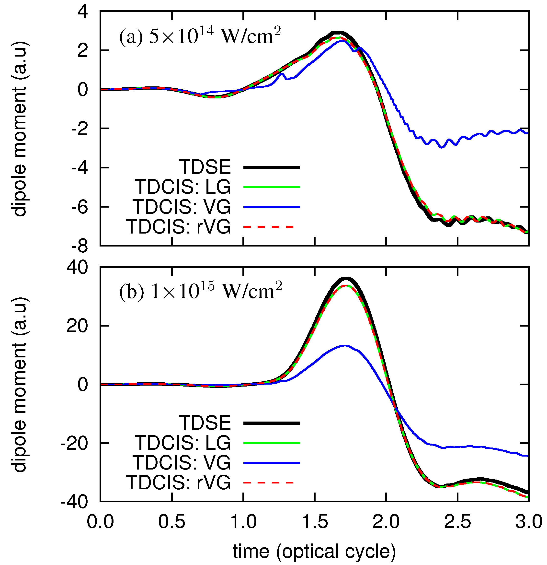
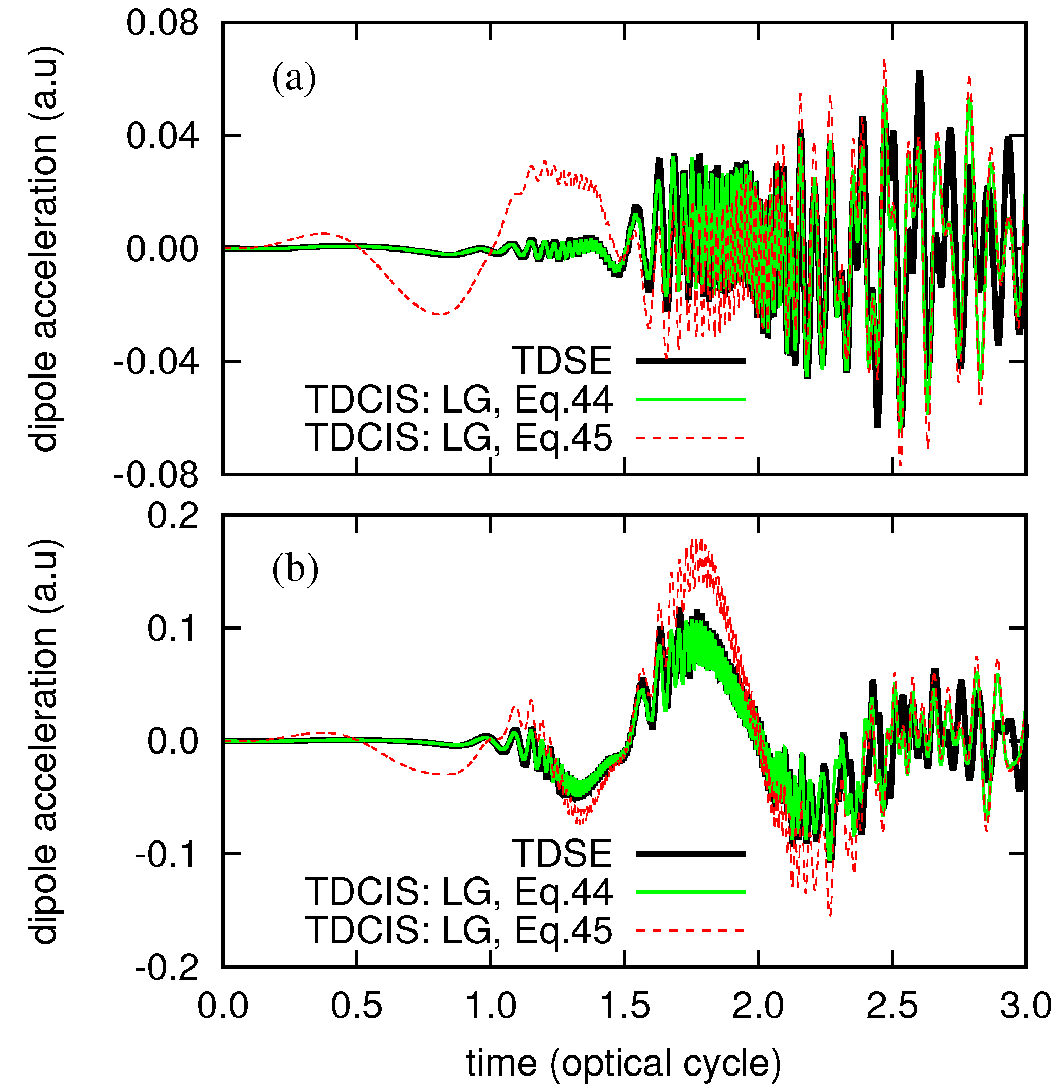
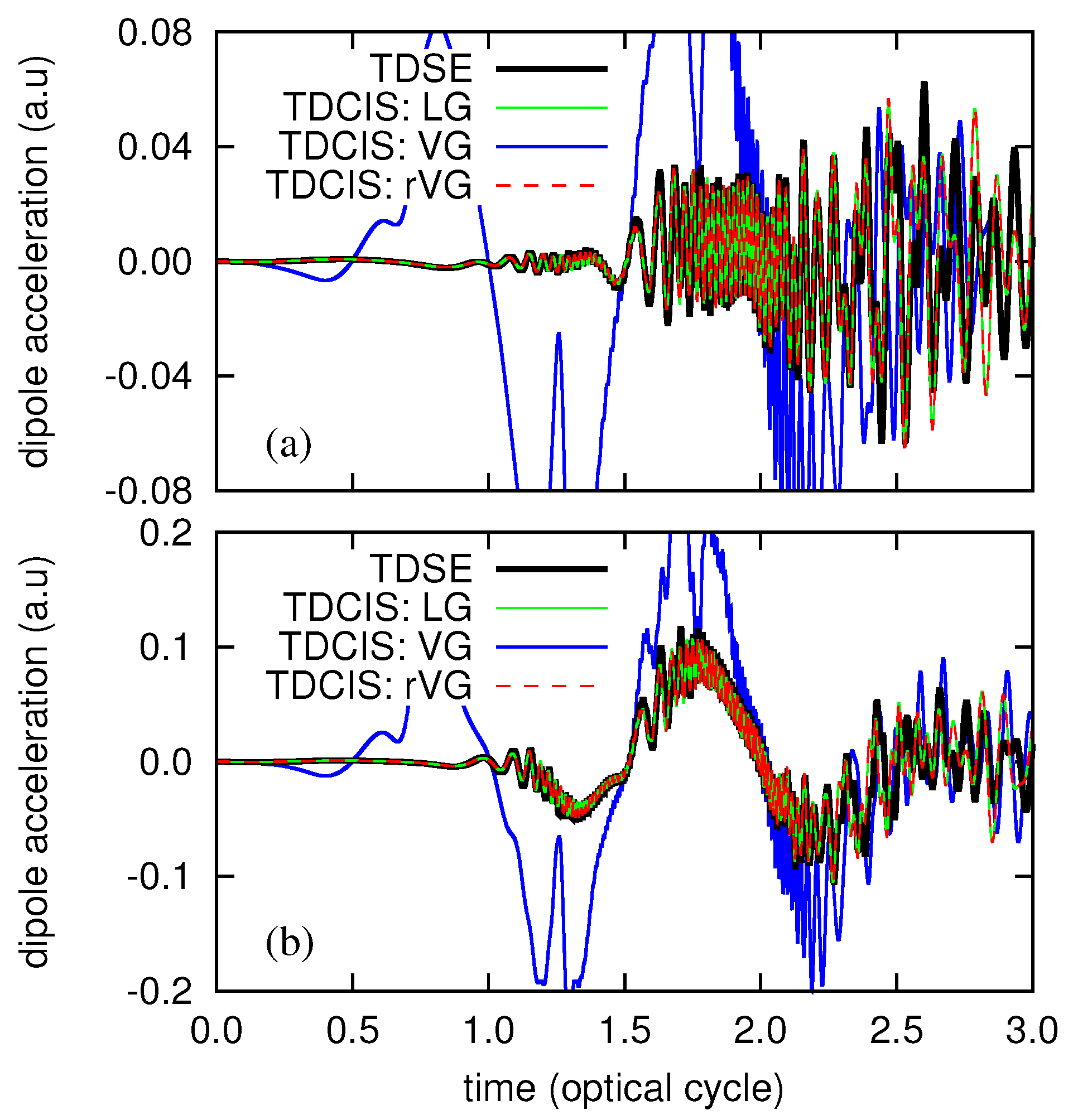
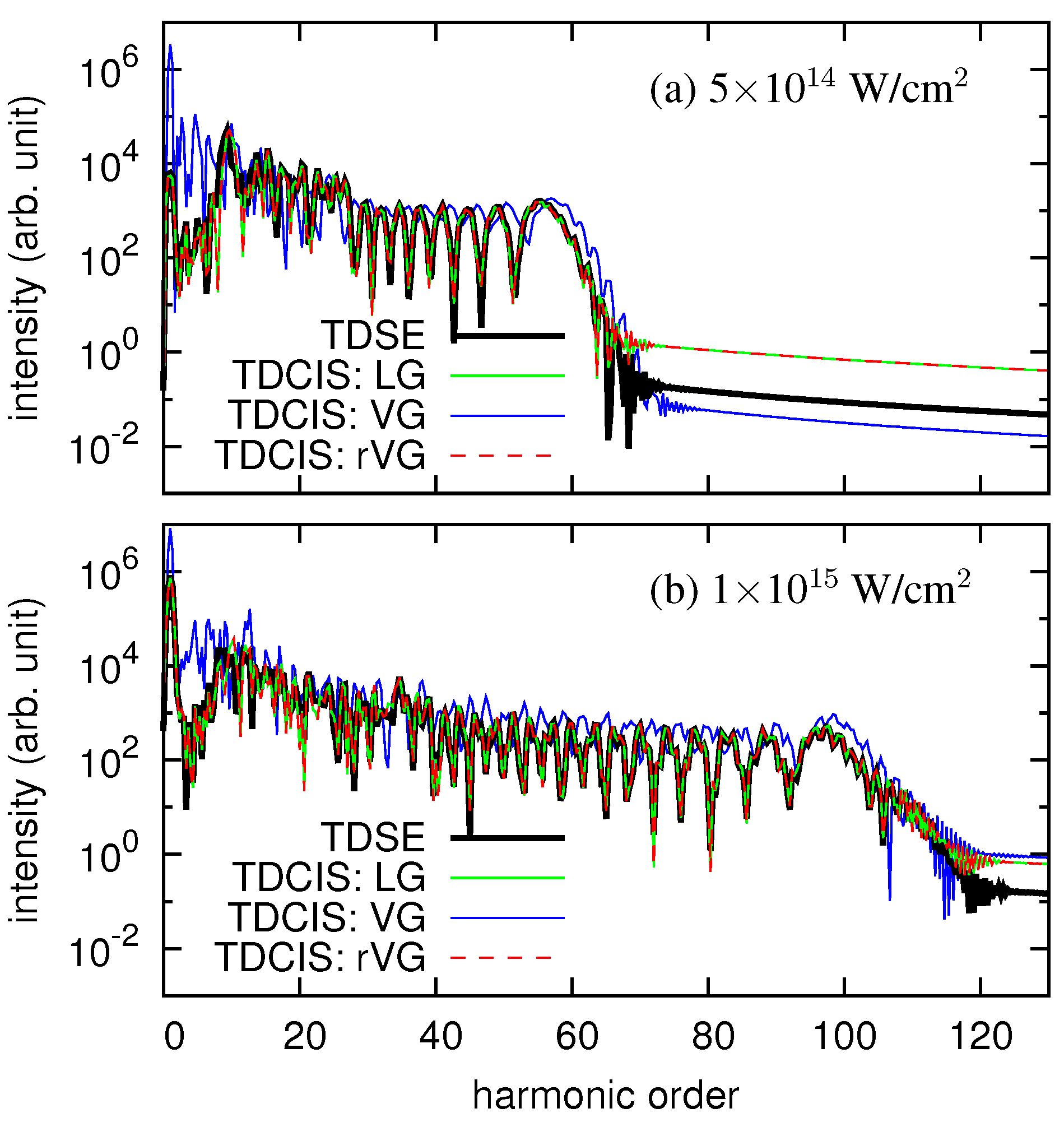
3. Numerical Examples

In this section, we numerically apply the channel orbital-based TDCIS method in the LG, VG, and rVG to the 1D model Helium atom, using the computational code developed by modifying an existing TDHF code used in our previous work [30,33,48]. The field-free electronic Hamiltonian is given by
H 0 = k = 1 2 1 2 2 z k 2 2 z k 2 + 1 + 1 ( z 1 z 2 ) 2 + 1 ,
for two electronic coordinates z 1 and z 2 , and the laser-electron interaction E ( t ) · r and A ( t ) · p are replaced with E ( t ) z and A ( t ) p z = i A ( t ) / z , respectively, in Equations (28), (30) and (37). Orbitals are discretized on equidistant grid points with spacing Δ z = 0.4 within a simulation box 1000 z 1000 , with an absorbing boundary implemented by a mask function of cos 1 / 4 shape at 10% side edges of the box. Each EOM is solved by the fourth-order Runge-Kutta method with a fixed time step size (1/10,000 of an optical cycle). Spatial derivatives are evaluated by the eighth order finite difference method, and spatial integrations are performed by the trapezoidal rule. We consider a laser electric field given by
E ( t ) = E 0 sin ( ω 0 t ) sin 2 π t τ ,
for 0 t τ , and E ( t ) = 0 otherwise, with a wavelength λ = 2 π / ω 0 = 750 nm, a foot-to-foot pulse length τ of three optical cycles, and a peak intensity I 0 = E 0 2 for I 0 = 5 × 10 14 W/cm 2 and I 0 = 10 15 W/cm 2 . The 1D Hamiltonian, computational details, and the applied laser field are the same as used in Ref. [48] to facilitate comparison with TDSE results in Ref. [48].
First, we compare the time-dependent dipole moment z ( t ) = Ψ ( t ) | ( z 1 + z 2 ) | Ψ ( t ) obtained with TDCIS approaches with that of TDSE in Figure 1, which immediately reveals a strong gauge dependence of fixed-orbital approaches, i.e., the large difference between LG and VG results. One should note that the comparison of LG and VG results alone can tell nothing about the preference of either approach; TDCIS method in both LG and VG are the first approximation in the hierarchy of CI expansions, which, at the full-CI limit, would be gauge invariant. The point here is that the LG scheme outperforms the VG scheme in comparison to the exact TDSE result as clearly seen in Figure 1, which convinces one of an empirical preference of the LG treatment. On the other hand, the results of LG and rVG agree perfectly within the graphical resolution, numerically demonstrating the theoretical gauge invariance.
Next, we consider the dipole acceleration a ( t ) defined as the time derivative of the kinematic momentum,
a ( t ) = d π d t ,
where π = Ψ | ( p z 1 + p z 2 ) | Ψ for the LG, and π = Ψ | ( p z 1 + p z 2 ) | Ψ + 2 A ( t ) for the VG. In the exact TDSE case, applying Equation (38) for O ^ = p ^ z proves that a = a Ehrenfest , with
a Ehrenfest ( t ) = Ψ | v nuc z 1 + v nuc z 2 | Ψ 2 E ( t ) ,
where v nuc / z = / z 2 ( z 2 + 1 ) 1 / 2 = 2 z ( z 2 + 1 ) 3 / 2 for the 1D Hamiltonian. Numerically achieving the theoretical equivalence of Equations (44) and (45), even for the exact TDSE method, requires a simulation to be converged with respect to computational parameters (time-step size, etc.). Therefore, we first applied both Equations (44) and (45) in the TDSE simulation, and confirmed a perfect agreement (not shown), suggesting the convergence of the simulation. Then we compare the results of TDCIS in the LG, using Equations (44) (i.e., Equation (40) with O ^ = p ^ z ) and (45), with that of TDSE in Figure 2, clearly showing a better agreement of the results of the former approach with that of TDSE. From this result, and also by the fact that being based on Equation (44) guarantees that the high-harmonic generation (HHG) spectra obtained from the velocity π ( t ) and the acceleration a ( t ) , at the convergence, properly relate to each other [45], we consider that Equation (44), together with Equation (40) or Equation (41), should be adopted as a consistent method for evaluating the dipole acceleration.
Then we compare the time evolution of the dipole acceleration (Figure 3) and the HHG spectrum (Figure 4) obtained as the modulus squared of the Fourier transform of the dipole acceleration obtained with TDCIS method in LG, VG, and rVG (based on Equation (44)) with those of TDSE. We observe that (1) the LG and rVG results are identical to each other within the scale of the figure, (2) they also show a good agreement with TDSE results, (3) and in contract, the VG results strongly deviate from all the other results. Especially, Figure 4 shows a remarkable agreement of the TDCIS spectra in the LG and rVG and the TDSE one, suggesting that the TDCIS method would be a useful computational method for studying HHG process in more complex atoms and molecules, in particular, when the present rVG treatment is combined with advanced, velocity gauge-specific computational techniques.

4. Conclusions

In this work, we propose a gauge-invariant formulation of the channel orbital-based TDCIS method for ab initio investigations of electron dynamics in atoms and molecules. Instead of using fixed orbitals both in length-gauge and velocity-gauge simulations, we adopt, in the velocity-gauge case, the EOMs derived with unitary rotated orbitals | ϕ p ( t ) = U ^ ( t ) | ϕ p using gauge-transforming operator U ^ ( t ) , which replaces the length-gauge operator E · r appearing in the length-gauge EOMs with the velocity-gauge counterpart A · p , while retaining the equivalence to the length-gauge treatment. This would make it possible to take advantages of the velocity-gauge simulation over the length-gauge one, e.g., the faster convergence of simulations of atoms interacting with an intense and/or long-wavelength laser field, with respect to the maximum angular momentum included to expand orbitals, and the native feasibility of advanced absorbing boundaries such as the exterior complex scaling. Numerical assessment of the present method for real atoms and molecules with the three-dimensional Hamiltonian will be presented elsewhere.

Acknowledgments

We thank Yuki Orimo for carefully reading the manuscript. This research was supported in part by a Grant-in-Aid for Scientific Research (Grants No. 26390076, No. 26600111, No. 16H03881, and 17K05070) from the Ministry of Education, Culture, Sports, Science and Technology (MEXT) of Japan and also by the Photon Frontier Network Program of MEXT. This research was also partially supported by the Center of Innovation Program from the Japan Science and Technology Agency, JST, and by CREST (Grant No. JPMJCR15N1), JST.

Author Contributions

Takeshi Sato conceived the idea. Takeshi Sato and Takuma Teramura formulated the method. Takeshi Sato numerically implemented the method and performed simulations. Takeshi Sato and Kenichi L. Ishikawa analyzed the results and co-wrote the original and revised manuscripts.

Conflicts of Interest

The authors declare no conflict of interest.

References

  1. Gordon, A.; Kärtner, F.X.; Rohringer, N.; Santra, R. Role of Many-Electron Dynamics in High Harmonic Generation. Phys. Rev. Lett. 2006, 96, 223902. [Google Scholar] [CrossRef] [PubMed]
  2. Rohringer, N.; Gordon, A.; Santra, R. Configuration-interaction-based time-dependent orbital approach for ab initio treatment of electronic dynamics in a strong optical laser field. Phys. Rev. A 2006, 74, 043420. [Google Scholar] [CrossRef]
  3. Rohringer, N.; Santra, R. Multichannel coherence in strong-field ionization. Phys. Rev. A 2009, 79, 053402. [Google Scholar] [CrossRef]
  4. Greenman, L.; Ho, P.J.; Pabst, S.; Kamarchik, E.; Mazziotti, D.A.; Santra, R. Implementation of the time-dependent configuration-interaction singles method for atomic strong-field processes. Phys. Rev. A 2010, 82, 023406. [Google Scholar]
  5. Pabst, S.; Greenman, L.; Ho, P.J.; Mazziotti, D.A.; Santra, R. Decoherence in Attosecond Photoionization. Phys. Rev. Lett. 2011, 106, 053003. [Google Scholar] [CrossRef] [PubMed]
  6. Pabst, S.; Greenman, L.; Mazziotti, D.A.; Santra, R. Impact of multichannel and multipole effects on the Cooper minimum in the high-order-harmonic spectrum of argon. Phys. Rev. A 2012, 85, 023411. [Google Scholar] [CrossRef]
  7. Sytcheva, A.; Pabst, S.; Son, S.K.; Santra, R. Enhanced nonlinear response of Ne8+ to intense ultrafast X rays. Phys. Rev. A 2012, 85, 023414. [Google Scholar] [CrossRef]
  8. Pabst, S.; Sytcheva, A.; Moulet, A.; Wirth, A.; Goulielmakis, E.; Santra, R. Theory of attosecond transient-absorption spectroscopy of krypton for overlapping pump and probe pulses. Phys. Rev. A 2012, 86, 063411. [Google Scholar]
  9. Pabst, S.; Santra, R. Strong-Field Many-Body Physics and the Giant Enhancement in the High-Harmonic Spectrum of Xenon. Phys. Rev. Lett. 2013, 111, 233005. [Google Scholar] [CrossRef] [PubMed]
  10. Pabst, S. Atomic and molecular dynamics triggered by ultrashort light pulses on the atto- to picosecond time scale. Eur. Phys. J. Spec. Top. 2013, 221, 1–71. [Google Scholar] [CrossRef]
  11. Heinrich-Josties, E.; Pabst, S.; Santra, R. Controlling the 2p hole alignment in neon via the 2s–3p Fano resonance. Phys. Rev. A 2014, 89, 043415. [Google Scholar] [CrossRef]
  12. Pabst, S.; Santra, R. Spin-orbit effects in atomic high-harmonic generation. J. Phys. B At. Mol. Opt. Phys. 2014, 47, 124026. [Google Scholar] [CrossRef]
  13. Hollstein, M.; Pfannkuche, D. Multielectron dynamics in the tunneling ionization of correlated quantum systems. Phys. Rev. A 2015, 92, 053421. [Google Scholar] [CrossRef]
  14. You, J.A.; Rohringer, N.; Dahlströ, J.M. Attosecond photoionization dynamics with stimulated core-valence transitions. Phys. Rev. A 2016, 93, 033413. [Google Scholar] [CrossRef]
  15. You, J.A.; Dahlströ, J.M.; Rohringer, N. Attosecond dynamics of light-induced resonant hole transfer in high-order-harmonic generation. Phys. Rev. A 2017, 95, 023409. [Google Scholar] [CrossRef]
  16. Grosser, M.; Slowik, J.M.; Santra, R. Attosecond X-ray scattering from a particle-hole wave packet. Phys. Rev. A 2017, 95, 062107. [Google Scholar] [CrossRef]
  17. Krebs, D.; Pabst, S.; Santra, R. Introducing many-body physics using atomic spectroscopy. Am. J. Phys. 2014, 82, 113. [Google Scholar] [CrossRef]
  18. Karamatskou, A.; Pabst, S.; Chen, Y.J.; Santra, R. Calculation of photoelectron spectra within the time-dependent configuration-interaction singles scheme. Phys. Rev. A 2014, 89, 033415. [Google Scholar] [CrossRef]
  19. Chen, Y.J.; Pabst, S.; Karamatskou, A.; Santra, R. Theoretical characterization of the collective resonance states underlying the xenon giant dipole resonance. Phys. Rev. A 2015, 91, 032503. [Google Scholar] [CrossRef]
  20. Tilley, M.; Karamatskou, A.; Santra, R. Wave-packet propagation based calculation of above-threshold ionization in the X-ray regime. J. Phys. B At. Mol. Opt. Phys. 2015, 48, 124001. [Google Scholar] [CrossRef]
  21. Karamatskou, A.; Pabst, S.; Chen, Y.J.; Santra, R. Erratum: Calculation of photoelectron spectra within the time-dependent configuration-interaction singles scheme [Phys. Rev. A 89, 033415 (2014)]. Phys. Rev. A 2015, 91, 069907(E). [Google Scholar] [CrossRef]
  22. Goetz, R.E.; Karamatskou, A.; Santra, R.; Koch, C.P. Quantum optimal control of photoelectron spectra and angular distributions. Phys. Rev. A 2016, 93, 013413. [Google Scholar] [CrossRef]
  23. Karamatskou, A.; Santra, R. Time-dependent configuration-interaction-singles calculation of the 5p-subshell two-photon ionization cross section in xenon. Phys. Rev. A 2017, 95, 013415. [Google Scholar] [CrossRef]
  24. Karamatskou, A. Nonlinear effects in photoionization over a broad photon-energy range within the TDCIS scheme. J. Phys. B At. Mol. Opt. Phys. 2017, 50, 013002. [Google Scholar] [CrossRef]
  25. Ishikawa, K.L.; Sato, T. A Review on Ab Initio Approaches for Multielectron Dynamics. IEEE J. Sel. Top. Quantum Electron. 2015, 21, 8700916. [Google Scholar] [CrossRef]
  26. Zanghellini, J.; Kitzler, M.; Fabian, C.; Brabec, T.; Scrinzi, A. An MCTDHF Approach to Multielectron Dynamics in Laser Fields. Laser Phys. 2003, 13, 1064. [Google Scholar]
  27. Kato, T.; Kono, H. Time-dependent multiconfiguration theory for electronic dynamics of molecules in an intense laser field. Chem. Phys. Lett. 2004, 392, 533. [Google Scholar] [CrossRef]
  28. Caillat, J.; Zanghellini, J.; Kitzler, M.; Koch, O.; Kreuzer, W.; Scrinzi, A. Correlated multielectron systems in strong laser fields: A multiconfiguration time-dependent Hartree-Fock approach. Phys. Rev. A 2005, 71, 012712. [Google Scholar] [CrossRef]
  29. Miyagi, H.; Madsen, L.B. Time-dependent restricted-active-space self-consistent-field theory for laser-driven many-electron dynamics. Phys. Rev. A 2013, 87, 062511. [Google Scholar] [CrossRef]
  30. Sato, T.; Ishikawa, K.L. Time-dependent complete-active-space self-consistent-field method for multielectron dynamics in intense laser fields. Phys. Rev. A 2013, 88, 023402. [Google Scholar] [CrossRef]
  31. Miyagi, H.; Madsen, L.B. Time-dependent restricted-active-space self-consistent-field theory for laser-driven many-electron dynamics. II. Extended formulation and numerical analysis. Phys. Rev. A 2014, 89, 063416. [Google Scholar] [CrossRef]
  32. Haxton, D.J.; McCurdy, C.W. Two methods for restricted configuration spaces within the multiconfiguration time-dependent Hartree-Fock method. Phys. Rev. A 2015, 91, 012509. [Google Scholar] [CrossRef]
  33. Sato, T.; Ishikawa, K.L. Time-dependent multiconfiguration self-consistent-field method based on occupation restricted multiple active space model for multielectron dynamics in intense laser fields. Phys. Rev. A 2015, 91, 023417. [Google Scholar] [CrossRef]
  34. Burke, P.G.; Burke, V.M. Time-dependent R-matrix theory of multiphoton processes. J. Phys. B 1997, 30, L383–L391. [Google Scholar] [CrossRef]
  35. Lysaght, M.A.; Burke, P.G.; van der Hart, H.W. Ultrafast Laser-Driven Excitation Dynamics in Ne: An Ab Initio Time-Dependent R-Matrix Approach. Phys. Rev. Lett. 2008, 101, 253001. [Google Scholar] [CrossRef] [PubMed]
  36. Lysaght, M.A.; van der Hart, H.W.; Burke, P.G. Time-dependent R-matrix theory for ultrafast atomic processes. Phys. Rev. A 2009, 79, 053411. [Google Scholar] [CrossRef]
  37. Lackner, F.; Břesinová, I.; Sato, T.; Ishikawa, K.L.; Burgdörfer, J. Propagating two-particle reduced density matrices without wave functions. Phys. Rev. A 2015, 91, 023412. [Google Scholar] [CrossRef]
  38. Lackner, F.; Břesinová, I.; Sato, T.; Ishikawa, K.L.; Burgdörfer, J. High-harmonic spectra from time-dependent two-particle reduced-density-matrix theory. Phys. Rev. A 2017, 95, 033414. [Google Scholar] [CrossRef]
  39. Nurhuda, M.; Faisal, F.H.M. Numerical solution of time-dependent Schrödinger equation for multiphoton processes: A matrix iterative method. Phys. Rev. A 1999, 60, 3125. [Google Scholar] [CrossRef]
  40. Grum-Grzhimailo, A.N.; Abeln, B.; Bartschat, K.; Weflen, D. Ionization of atomic hydrogen in strong infrared laser fields. Phys. Rev. A 2010, 81, 043408. [Google Scholar] [CrossRef]
  41. Sato, T.; Ishikawa, K.L.; Břesinová, I.; Lackner, F.; Burgdörfer, J. Time-dependent complete-active-space self-consistent-field method for atoms: Application to high-harmonic generation. Phys. Rev. A 2016, 94, 023405. [Google Scholar] [CrossRef]
  42. Dahlstrom, J.M.; Pabst, S.; Lindroth, E. Attosecond transient absorption of a bound wave packet coupled to a smooth continuum. J. Opt. 2017, 19, 114004. [Google Scholar] [CrossRef]
  43. Scrinzi, A. Infinite-range exterior complex scaling as a perfect absorber in time-dependent problems. Phys. Rev. A 2010, 81, 053845. [Google Scholar] [CrossRef]
  44. Orimo, Y.; Sato, T.; Scrinzi, A.; Ishikawa, K.L. Implementation of infinite-range exterior complex scaling to the time-dependent complete-active-space self-consistent-field method. Phys. Rev. A 2018, 97, 023423. [Google Scholar] [CrossRef]
  45. Bandrauk, A.D.; Chelkowski, S.; Diestler, D.J.; Manz, J.; Yuan, K.J. Quantum simulation of high-order harmonic spectra of the hydrogen atom. Phys. Rev. A 2009, 79, 023403. [Google Scholar] [CrossRef]
  46. Han, Y.C.; Madsen, L.B. Comparison between length and velocity gauges in quantum simulations of high-order harmonic generation. Phys. Rev. A 2010, 81, 063430. [Google Scholar] [CrossRef]
  47. Bandrauk, A.D.; Fillion-Gourdeau, F.; Lorin, E. Atoms and molecules in intense laser fields: Gauge invariance of theory and models. J. Phys. B At. Mol. Opt. Phys. 2013, 46, 153001. [Google Scholar] [CrossRef]
  48. Sato, T.; Ishikawa, K.L. The structure of approximate two electron wavefunctions in intense laser driven ionization dynamics. J. Phys. B At. Mol. Opt. Phys. 2014, 47, 204031. [Google Scholar] [CrossRef]
Figure 1. Time evolution of the dipole moment of 1D-He exposed to a laser pulse with a wavelength of 750 nm and an intensity of (a) 5 × 10 14 W/cm 2 and (b) 1 × 10 15 W/cm 2 . Comparison of the results with time-dependent configuration interaction singles (TDCIS) in the length gauge (LG), velocity gauge (VG), and rotated velocity-gauge (rVG) with that of the time-dependent Schrödinger equation (TDSE).
Applsci 08 00433 g001
Figure 2. Time evolution of the dipole acceleration of 1D-He exposed to a laser pulse with a wavelength of 750 nm and an intensity of (a) 5 × 10 14 W/cm 2 and (b) 1 × 10 15 W/cm 2 . Comparison of the results with TDCIS in the LG adopting Equations (44) and (45) with that of TDSE.
Applsci 08 00433 g002
Figure 3. Time evolution of the dipole acceleration of 1D-He exposed to a laser pulse with a wavelength of 750 nm and an intensity of (a) 5 × 10 14 W/cm 2 and (b) 1 × 10 15 W/cm 2 . Comparison of the results with TDCIS in the LG, VG, and rVG with that of TDSE.
Applsci 08 00433 g003
Figure 4. High-harmonic spectrum of 1D-He exposed to a laser pulse with a wavelength of 750 nm and an intensity of (a) 5 × 10 14 W/cm 2 and (b) 1 × 10 15 W/cm 2 . Comparison of the results with TDCIS in the LG, VG, and rVG with that of TDSE.
Applsci 08 00433 g004

