Object Tracking with LiDAR: Monitoring Taxiing and Landing Aircraft


Department of Civil, Environmental and Geodetic Engineering, The Ohio State University, 470 Hitchcock Hall, 2070 Neil Ave, Columbus, OH 43210, USA
*
Author to whom correspondence should be addressed.
Appl. Sci. 2018, 8(2), 234; https://doi.org/10.3390/app8020234
Submission received: 16 January 2018
/
Revised: 31 January 2018
/
Accepted: 1 February 2018
/
Published: 3 February 2018
(This article belongs to the Special Issue Laser Scanning)
Abstract
:Featured Application
Tracking aircraft during taxiing, landing and takeoffs at airports; acquiring statistical data for centerline deviation analysis and veer-off modeling as well as for airport design in general.
Abstract
Mobile light detection and ranging (LiDAR) sensors used in car navigation and robotics, such as the Velodyne’s VLP-16 and HDL-32E, allow for sensing the surroundings of the platform with high temporal resolution to detect obstacles, tracking objects and support path planning. This study investigates the feasibility of using LiDAR sensors for tracking taxiing or landing aircraft close to the ground to improve airport safety. A prototype system was developed and installed at an airfield to capture point clouds to monitor aircraft operations. One of the challenges of accurate object tracking using the Velodyne sensors is the relatively small vertical field of view (30°, 41.3°) and angular resolution (1.33°, 2°), resulting in a small number of points of the tracked object. The point density decreases with the object–sensor distance, and is already sparse at a moderate range of 30–40 m. The paper introduces our model-based tracking algorithms, including volume minimization and cube trajectories, to address the optimal estimation of object motion and tracking based on sparse point clouds. Using a network of sensors, multiple tests were conducted at an airport to assess the performance of the demonstration system and the algorithms developed. The investigation was focused on monitoring small aircraft moving on runways and taxiways, and the results indicate less than 0.7 m/s and 17 cm velocity and positioning accuracy achieved, respectively. Overall, based on our findings, this technology is promising not only for aircraft monitoring but for airport applications.
1. Introduction
Remote sensing technologies have long been used for mapping the static part of natural and man-made environments, including the shape of the Earth, transportation infrastructure, and buildings. As sensing technologies continue to advance, more powerful remote sensing systems have been developed [1], allowing us to observe and monitor the dynamic components of the environment. Light detection and ranging (LiDAR), as remote sensing technology, is already successfully applied to track pedestrian movements [2,3,4] and ground vehicle traffic from stationary [5] or on-board sensors [6,7].
Similar to ground vehicle or pedestrian traffic monitoring, airfield operations, such as taxiing, takeoffs and landings, can be observed and tracked using LiDAR sensors installed on the airfield. Safety at airports is a serious concern worldwide, since 30% of fatal accidents occurred during landing and takeoff and 10% during taxiing or other ground operations between 2007 and 2016 based on the Boeing Company’s annual report [8]. Aircrafts motion around airports are tracked by RADAR, but airfield surveillance primarily relies on human observations from control towers. Clearly, active remote sensing in general is able to reduce the human error factor and operates in 24/7 in bad visibility conditions [9]. This feasibility study examines the achievable accuracy of a LiDAR-based monitoring system installed at an airfield to track and derive the trajectory of taxiing aircraft. At close range, LiDAR allows for directly capturing a more detailed and accurate 3D representation of taxiing or landing aircraft compared to existing radar or camera systems due to the higher spatial resolution. The 3D data enables accurately estimating driving patterns or trajectories, detecting aircraft types, monitoring aircraft operations in general, and can be applied to pilot education and training. Analysis of a large number of trajectories can be used for creating stochastic models of the airplane behavior during various operations, and this information can then be used for airport infrastructure and operation planning.
Various researchers have already investigated the LiDAR technology for improving airport safety [9,10], and our earlier studies [11,12] were the first attempt to use LiDAR sensors to track aircraft ground movements. As the continuation of our previous work, in this study, we apply a more complex sensor network, rigorously address the sensor georeferencing, and for the first time, track airplanes during landings. The main contribution of the paper is the introduction of a novel algorithm to derive motion parameters and extract the trajectory of objects from sparse point clouds. Unlike terrestrial laser scanners that are able to produce large and detailed point clouds over a long scan time, mobile LiDAR sensors applied in autonomous vehicle or robotic applications capture sparse point clouds, but with high temporal resolution; typically, at 10–30 Hz. These sensors make complete 360° scans around the rotation axis and capture data along multiple planes, producing high resolution in these planes. For instance, the Velodyne VLP-16 [13] and HDL-32E [14] LiDAR sensors, used in this study, have a 30° and 41.3° field of view, respectively, and the 16 and 32 planes represent an angular resolution of 1.33° and 2°, which much coarser than the 0.1°–0.3° resolution around the rotation axis. These sensor characteristics translate to only about 10–20 points per scan captured from a Cessna-sized airplane at a 40-m object–sensor distance. Note that the minimum distance to deploy sensors around runways and taxiways is regulated by the airport authorities for safety reasons. Clearly, the challenge is to track aircraft from these low-resolution LiDAR scans. The algorithm addressing this issue and presented in this paper could be of interest to autonomous vehicle applications or robotics to track objects that are farther away from the LiDAR sensor.
The structure of the paper is as follows. In the next “Background” subsection, the classification and brief description of the existing tracking algorithms, such as center of gravity (COG) and iterative closest point (ICP) approaches, are presented briefly. Then, Section 2 presents the hardware components of the demonstration system and the procedure for sensor georeferencing. This section also introduces the proposed algorithms to estimate the parameters of the underlying motion model from point clouds of low point density, including the details of the algorithms and the implementation challenges. In the Section 3, two tests are presented using the demonstration system installed at an airfield. During the two tests, data from taxiing and landing aircraft were captured. Section 4 presents the results of the two tests followed by Section 5 that provides the performance analysis, the comparison of the algorithms as well as the qualitative and quantitative error assessments. The papers ends with a conclusion and appendices. The terminology and most common definitions used throughout the paper can be found in Appendix A.
Background
LiDAR as well as other sensors used for tracking objects can be deployed on mobile or static platforms. The first case is the typical setup for mobile mapping, autonomous vehicles, and robotics. This is a challenging case, because the platform is moving, as is the tracked object, and consequently, the sensor has to be accurately georeferenced at all time. In contrast, the static setup is a simpler case, since the sensor georeferencing has to be done only once. This arrangement is commonly used in surveillance or transportation applications for traffic monitoring. In this study, the static sensor configuration is applied.
Several algorithms exist for tracking objects, such as pedestrians or vehicles, in 3D LiDAR data, and can be divided into model-free and model-based approaches according to Wang et al. [15]. The model-free approaches do not assume any properties, such as the shape of the object or motion model, which the tracked object is following. In contrast, model-based approaches use prior information regarding the object to achieve more reliable tracking. Obviously, model-free algorithms are more general, but model-based methods perform better. Methods introduced in this study are model-based and consider the type of the object assuming certain types of motion models.
The general workflow of the object tracking in point clouds includes object segmentation, recognition and tracking. The dynamic elements of each scan are separated from the static background during the segmentation step, then the object is recognized in the model-based approach [2,3]. Afterwards, the trajectory or motion parameters extracted from consecutive scans, and thus, the captured points from the moving objects, are known epoch-by-epoch. One can easily estimate the trajectory by calculating, for example, the center of gravity (COG) of the segmented points from each scan. Other solutions are based on point cloud registration algorithms. The iterative closest point (ICP) method [16] can be used to estimate, for instance, the six degrees of freedom (rigid body) transformation matrix between the consecutive and segmented scans (see for instance [17]). The transformation matrices contain the rotation and translation parameters that can be used for computing the trajectory. In another approach, instead of using the whole segmented scan, the common feature points or points sets can be extracted from the scans, and the transformation matrix is estimated based on these correspondences [18]. The tracking can be improved with considering the previous scans using Bayesian or Markov approaches [18,19], or the final trajectory can be refined with Kalman filtering or other smoothing techniques.
2. Prototype System and Methods
2.1. System Overview
The prototype sensor network consists of sensor stations, deployed along the runway or taxiway to be monitored. Sensor stations have Velodyne’s LiDAR sensors and a GPS antenna, rigidly attached to the column of a standard airport light fixture. Besides georeferencing, GPS provides accurate timing for the LiDAR sensors using the 1PPS (pulse per second) and NMEA (National Marine Electronic Association) GPS signals. In addition, each sensor station has a data logging component, deployed farther away from the runway or taxiway for safety reasons.
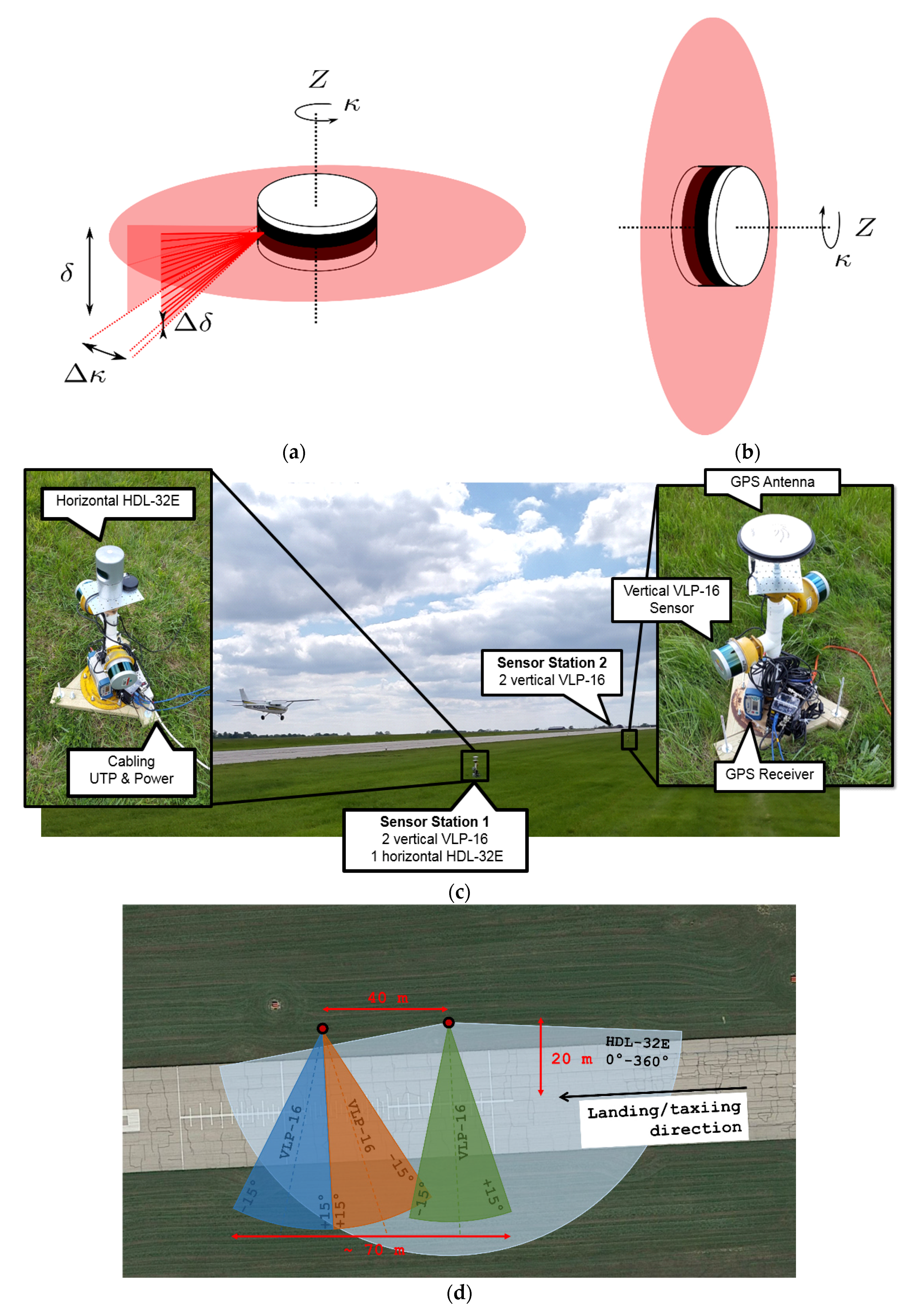
The adjustable sensor configuration allows for various sensor alignments. For example, Figure 1a,b show horizontally and vertically aligned VLP-16 sensors, respectively, where is the rotation axis and is the horizontal rotation angle or azimuth ranging from 0° to 360° with 0.1–0.3° angular resolution (). The vertical and horizontal alignments mean that the sensor’s rotation plane is either perpendicular or parallel to the horizontal plane, respectively. The narrower field of view () is 30° and 41.3° with 1.33° and 2° angular resolution () for the VLP-16 and HDL-32E systems, respectively. In an installation shown in Figure 1c, the left side shows two vertically aligned VLP-16s and one horizontally aligned HDL-32E scanner, while the right side shows two vertically aligned VLP-16 scanners.
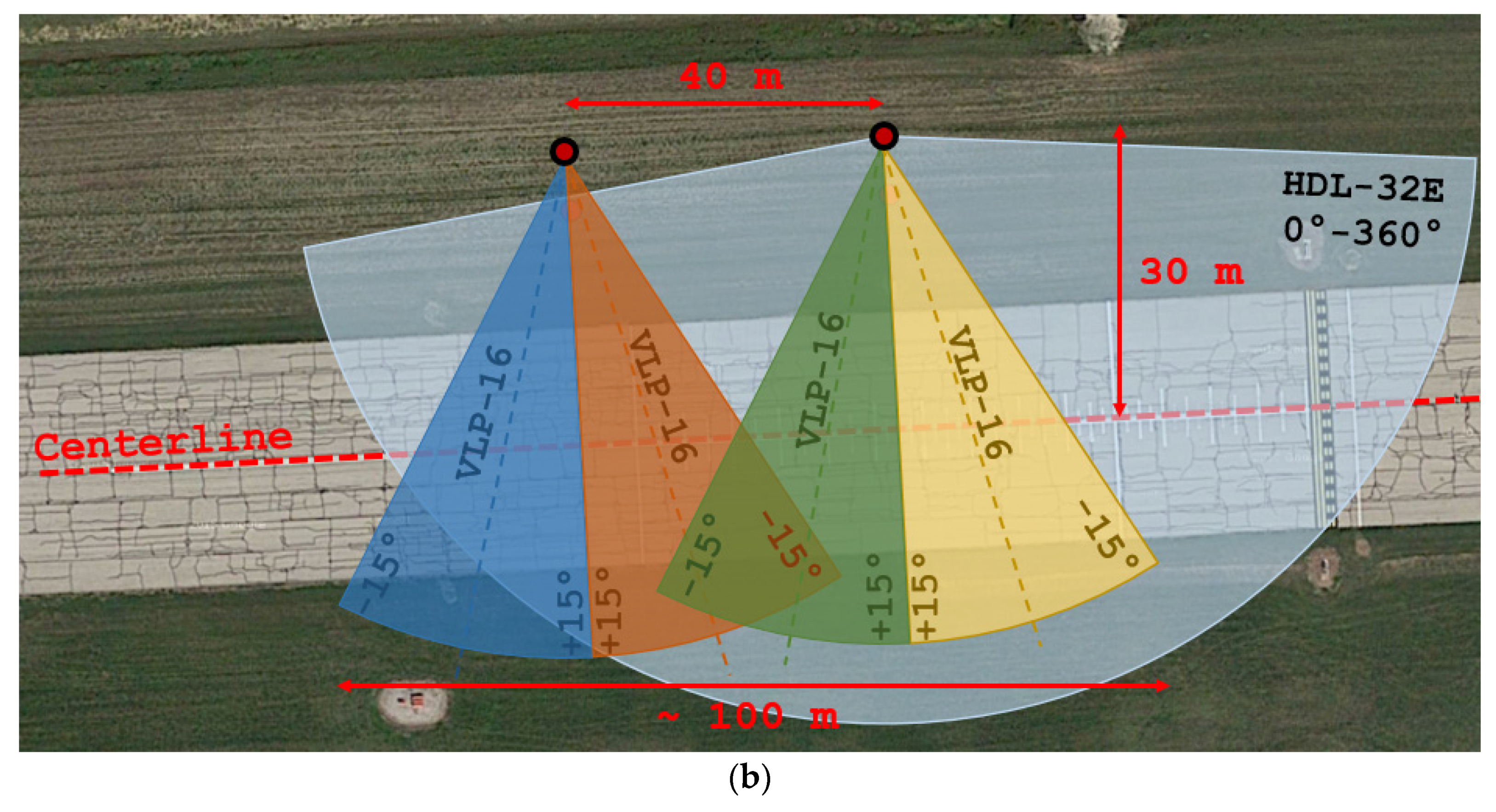
The alignment of the sensors was optimized to cover the largest field of view to capture the maximum number of points from the tracked object for a given number of scanners. A simulation study on this subject was conducted using Blender (see [12,20]). Since the Velodyne’s VLP-16 sensors have a smaller vertical field of view with coarser angular resolution, therefore these sensors are aligned vertically. While with this arrangement, the horizontal coverage of the runway is shorter, yet more points can be captured from the aircraft body. HDL-32E LiDAR is installed horizontally, due to its better vertical angular resolution and larger field of view. The minimum distance at the airport where our tests were conducted was specified as 20 m and 30 m next to taxiways and runways, respectively. The two sensor stations 40 m apart from each other provides an effective coverage of the runway of about 70 m (see Figure 1d).
2.2. Sensor Georeferencing
In a sensor network, point clouds acquired by the individual sensors have to be transformed into a common reference frame that could be local or global. When rigidly connected sensors are used together, then the coordinate system of one of the sensors is considered as a local frame, and the relative translation and rotation of the other sensors are estimated. This procedure is called point cloud co-registration. There are many co-registration approaches and most of these methods require a measurable overlap between point clouds that may not be feasible in the proposed system configuration here. Therefore, in contrast to co-registration, the coordinates and rotations of the sensors are independently estimated in a global system. This procedure is generally referred to as sensor georeferencing.
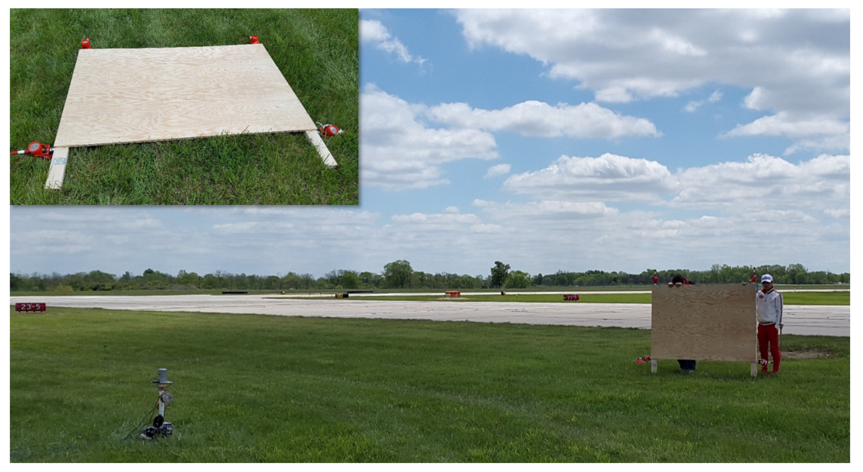
Sensor georeferencing includes the determination of the position and orientation in a reference frame. The coordinates of the LiDAR sensor location are measured with conventional land surveying technique using total station. The sensor orientation is usually indirectly estimated by using object space targets. In our case for estimating the three attitude angles, a 1.8 m x 1.2 m calibration board is used as a target (see Figure 2). This smooth and flat calibration board is large enough to provide a sufficient number of points obtained from it. Prisms attached to the four corners of the board were used to measure their global coordinates with a total station. The board was observed at various locations and orientations in the field of view of the sensors (see Figure 2).
The boresight estimation is based on comparing the total station measured target locations and orientations to the same parameters, estimated from the point clouds of the targets. Obviously, there is no chance that the prism locations are measured by the point cloud, but fitting a plane the orientation of the board surface can be estimated. Consequently, the norm vectors of the board in the sensor and global system can be calculated from the LiDAR points and the corner measurements, respectively. Using the two results, finding the unknown orientation parameters can be formulated as a least squares estimation problem:
where is the norm vector of the board in the global system at the th position, is the norm vector of the board in the sensor coordinate system at the th position, is the number of board positions, and is the rotation matrix as the function of the orientation parameters; for detailed notations and definitions see Appendix A. The Levenberg–Marquardt method is used to solve Equation (1). The positions and orientations of the sensors along with the time synchronization allow for transforming all points captured at different epochs to the same global coordinate system.
2.3. Aircraft Segmentation from LiDAR Scans
The first step of object tracking is the separation of the dynamic and static content of the scene, and then identification of the dynamic objects. A reference or baseline scan of the background can be obtained from scans that include no aircraft, and then, an occupancy grid is created from the average background scan. During tracking, this grid is compared to an incoming scan, and thus, the dynamic content could be easily filtered. The performance is further improved by defining a region of interest from the scans, such as the runway or taxiway in view.
In our tests, only one airplane presents at any epoch, and therefore, this segmentation is a relatively easy task. It is noteworthy that almost always just one plane is in the network’s field of view for landing scenarios due to mandatory aircraft separation. Obviously, there can be more than one plane in the case of taxiing. In the latter case, the airplanes can be segmented from each other by simply tracking their motion in the region of interest. At the end of the segmentation process, 3D coordinates of the aircraft body points with their timestamps are available for each scan.
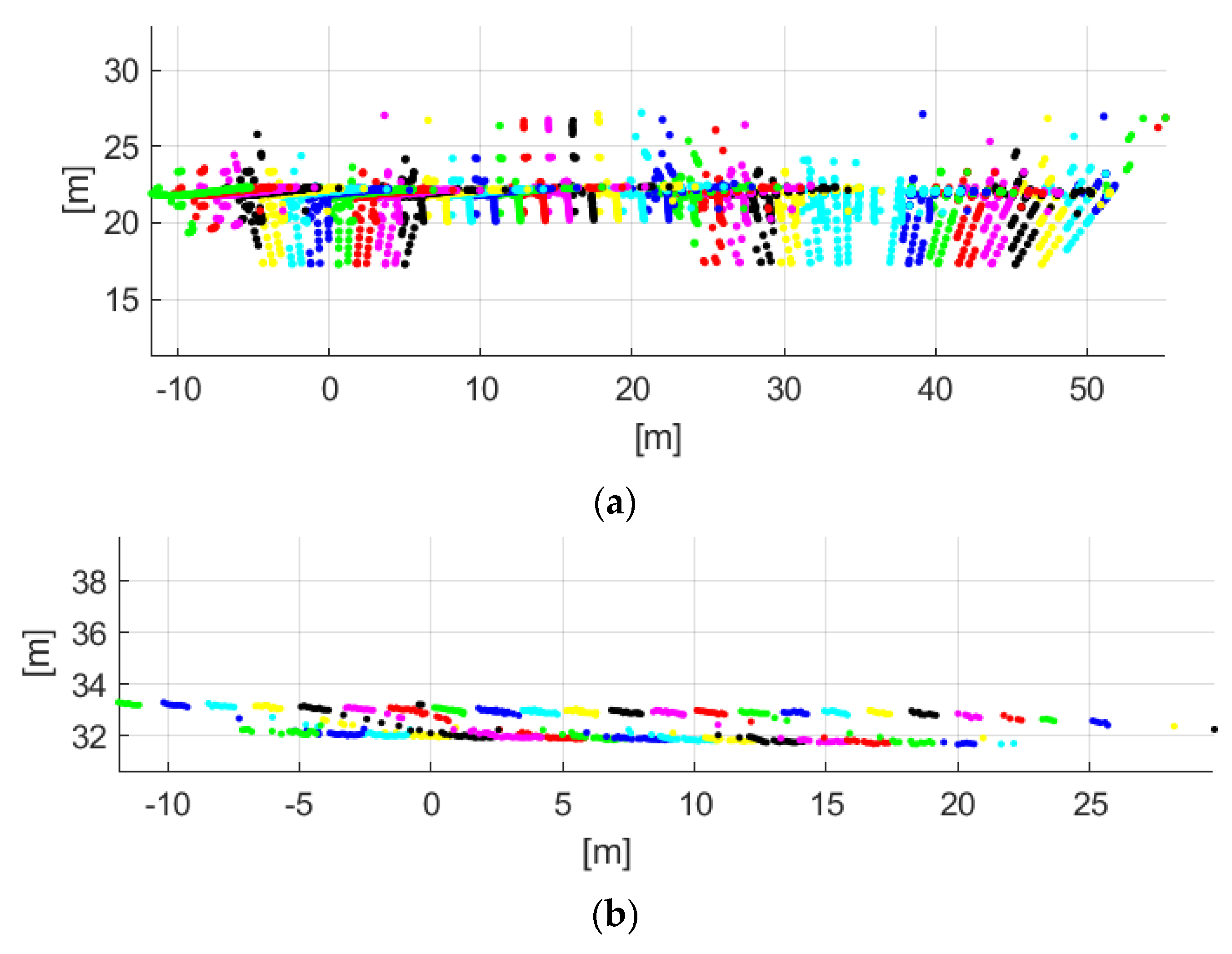
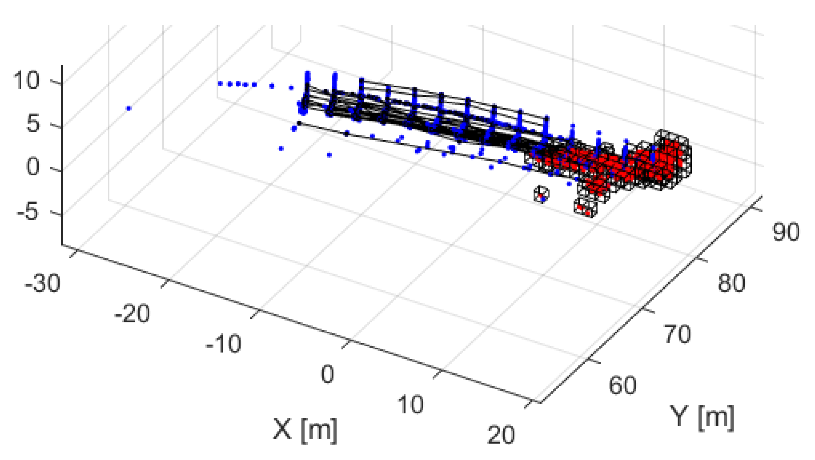
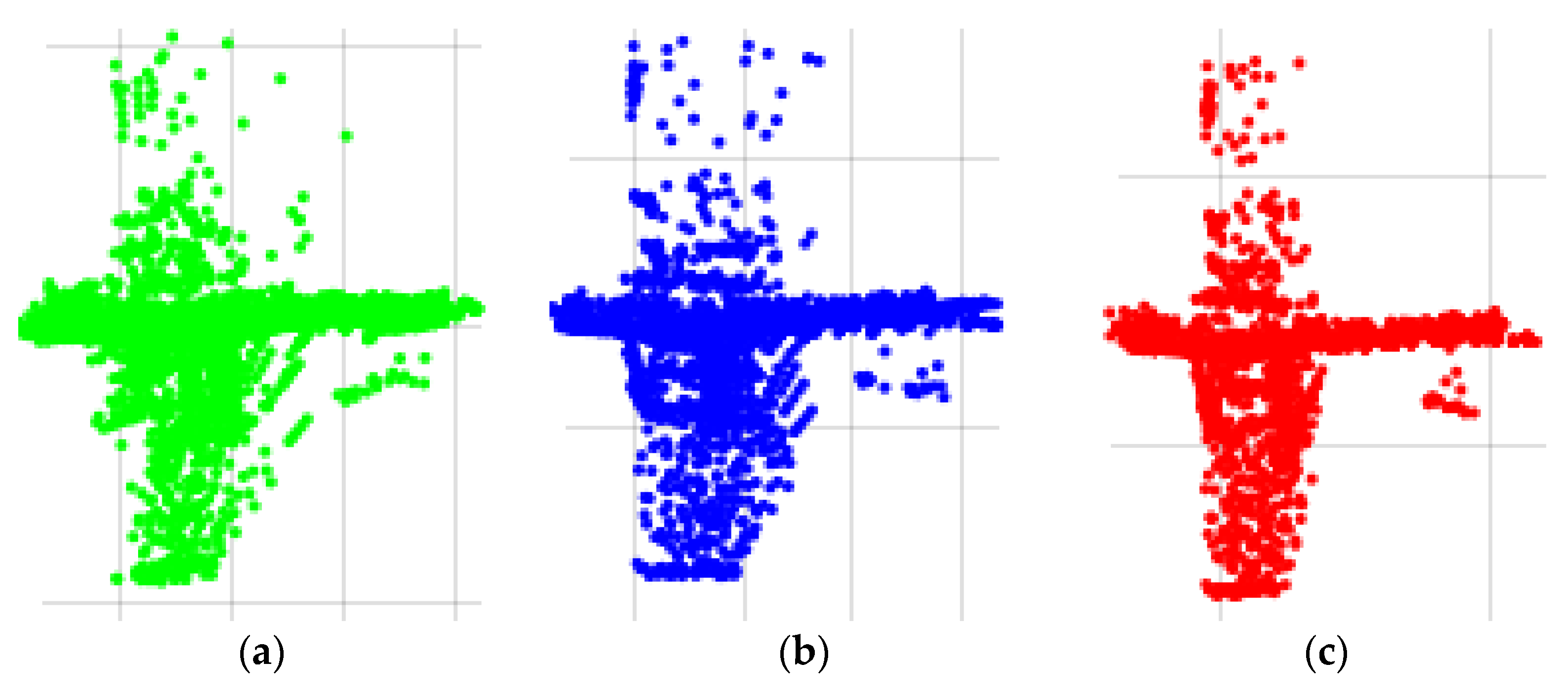
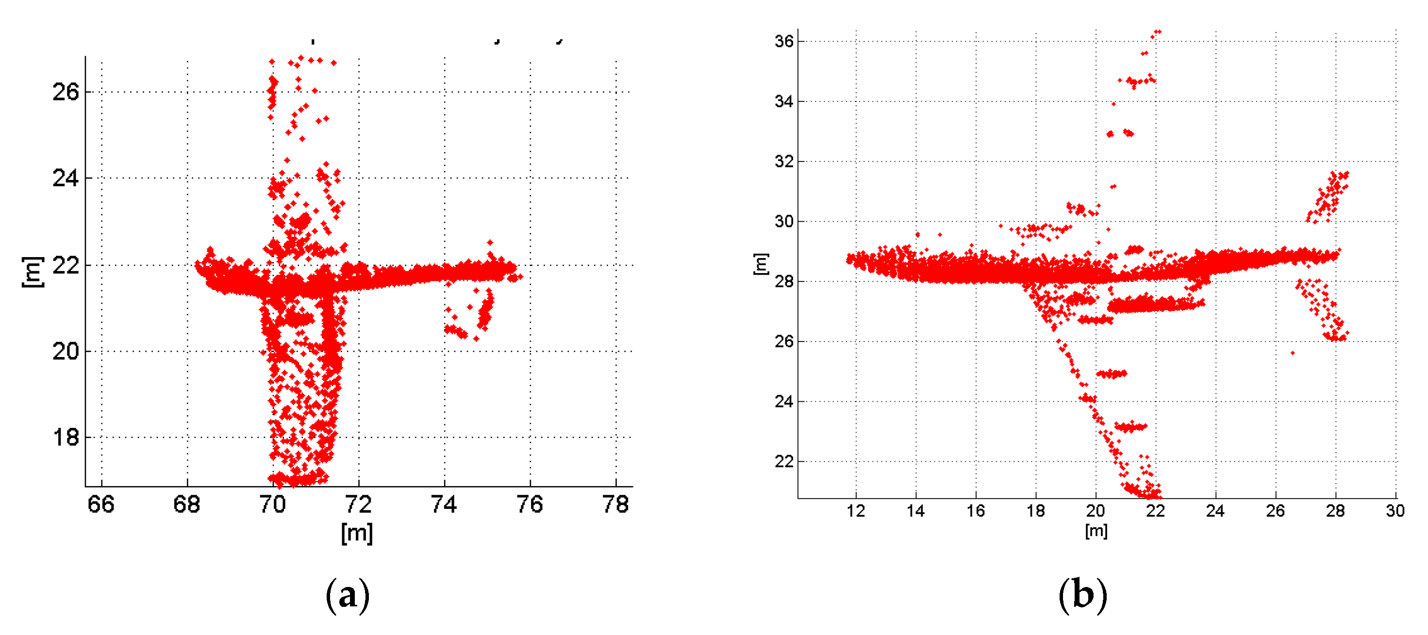
The density of the captured scans depends on the object–sensor distance. Figure 3 shows segmented data captured by five LiDAR sensors at 23 m and 33 m object–sensor distance. Various colors indicate the times, and thus, the point cloud in the figures shows all scans of the plane while crossing the sensor network’s field of view. Clearly, the shape of the airplane is barely recognizable in Figure 3a, and not recognizable in Figure 3b. These scans contain a very small number of points of the aircraft body due to the large object–sensor distance, and thus, dedicated algorithms are needed to extract the motion information or trajectories.
2.4. Motion Models
This study uses a model-based object tracking approach to address the issue of small number of captured points. Three types of motion models, namely, constant velocity (CV), constant acceleration (CA), and polynomial motion model, are used to describe the dynamics of taxiing or landing airplanes. The models for one coordinate axis are shown in Table 1; details of these models can be found in Appendix B. For all three models, the following two assumptions are made. First, the tracked plane follows a rigid body motion, and second, the heading of the aircraft body points towards the motion direction. The second condition is approximate for landing aircraft, as side wind may introduce an error in the heading and aircraft attitude. These assumptions mean that all points from the aircraft have the same motion parameters. The faster the aircraft moves the better the assumptions hold. We also assumes 2D motion for taxiing and 3D motion for landing. Note that, in the simplest case, the trajectory of the CV model is a straight line, and thus, the limitation of this model is that it cannot be used for tracking turns, accelerations or decelerations. However, this motion is still valid within a short time window. The CA model is able to describe more complex motion, namely curvilinear motion, but it is still inadequate to model sharp turns. The general or polynomial model allows for describing arbitrary trajectories besides the assumptions presented above.
2.5. Object Space Reconstruction with Various Motion Models
If the motion model is chosen and the parameters of the model, such as velocity, acceleration or the coefficients of the polynomial model are known, then all points of the aircraft body taken at different epochs can be transformed back to a common frame at zero time, resulting in a reconstructed point cloud—in other words, in the reconstruction of the aircraft body (see the end of Appendix B). Thus, the motion model with known parameters can be interpreted as a time-varying transformation. Figure 4 shows an example of the reconstruction assuming CV motion at 4.5, 6.5, 8.5 and 10.5 m/s velocities. Note that as the velocity parameter in the X direction approaches the real value, the reconstructed point cloud becomes sharper and more consistent, and finally, the aircraft body is clearly recognizable at 10.5 m/s. The idea behind the proposed approach of finding the motion parameters is to measure the consistency, or ‘order’, of the reconstruction. Obviously, if the motion parameters are known, the trajectory can be simply calculated using the model.
2.6. Estimating the Motion Model with Volume Minimization
The proposed algorithm, called volume minimization (VM), adjusts the motion parameters to find the optimal reconstruction that occupies the minimum volume of the reconstructed point cloud of the aircraft. In this way, the volume of the reconstruction is used as a metric for measuring the point cloud consistency:
where is a point from point cloud at time, depicts the motion model that transforms a point to epoch based on the underlying motion model with given motion parameters, and finally, is a function that measures the volume of a point cloud.
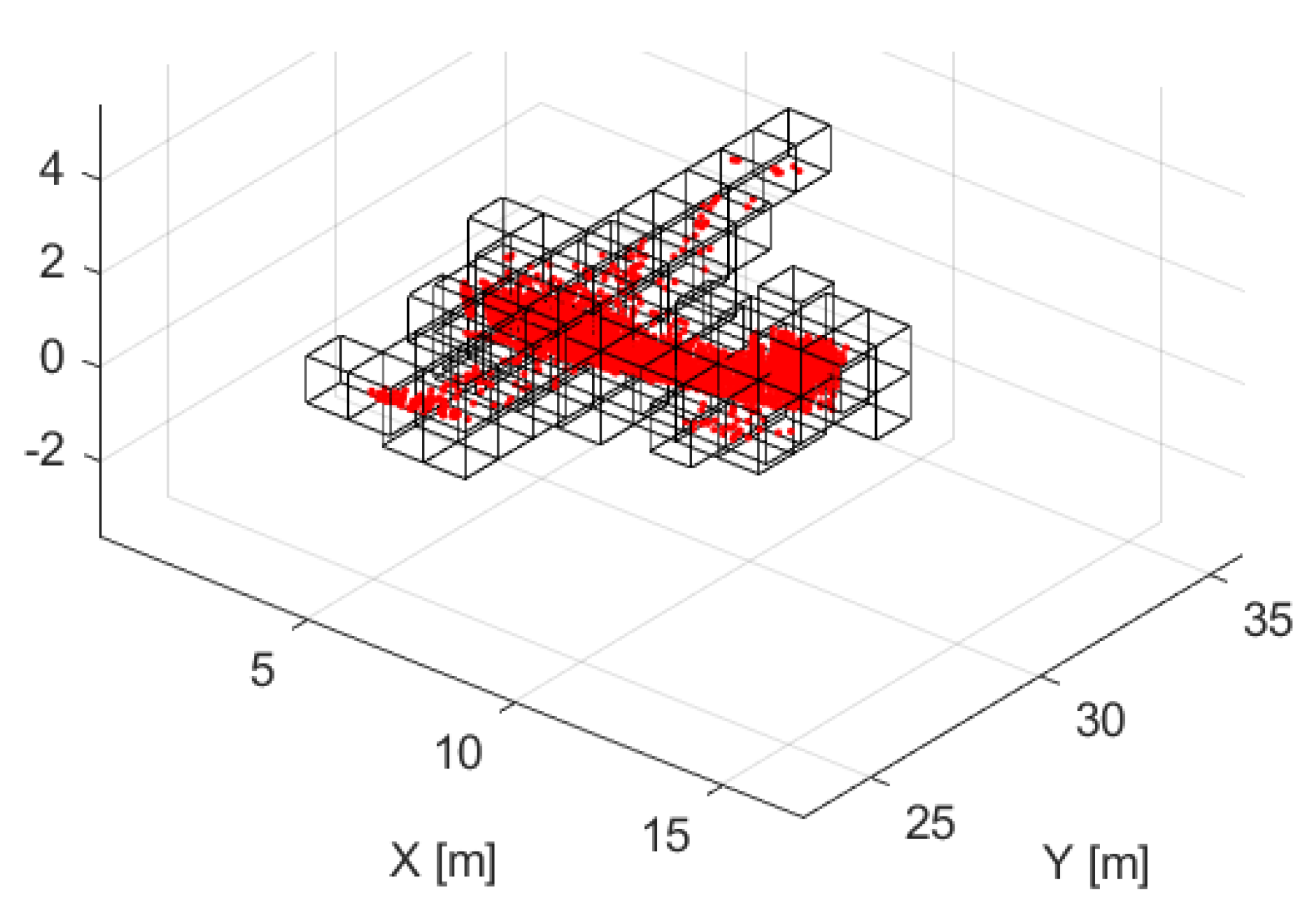
During volume minimization, the space is decimated into cubes, and the volume is measured by the number of cubes occupied by the reconstructed point cloud, as shown in Figure 5. Figure 4 shows the cubes from top view, and clearly illustrates that as the velocity approaches the real value, and the reconstruction becomes more realistic, the cube numbers also decrease, demonstrating that the proposed metric is consistent with the reconstruction quality. It is noteworthy that instead of volume, one can use entropy similar to [21,22]. For our dataset, we found that the volume as metric requires less computation and has better convergence properties as opposed to entropy.
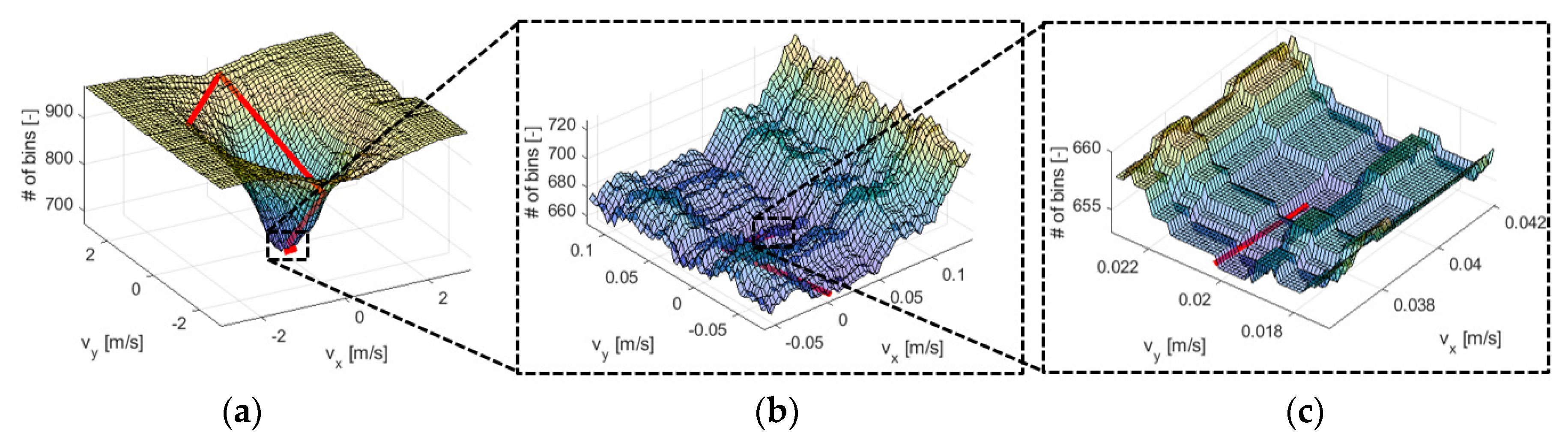
An objective function of Equation (2) for the CV model is presented in Figure 6 in order to analyze the problem space. Note that the figure shows the function at different scales. Although the objective function at large scale, shown in Figure 6a, seems quasi-convex, the medium scale in Figure 6b, reveals that this function is highly non-convex. The complexity of the objective function depends on the cube size, the number of points captured from the aircraft, and the applied motion model. Obviously, the objective function is non-smooth due to the volume calculation presented above. This can be clearly seen at small scale in Figure 6c, which shows that the objective function is a multivariate step function. Consequently, one possible solution can be to approximate the objective function with a smooth function to solve the problem with one of the smooth optimization techniques, which solution is very likely to be sub-optimal. Alternatively, non-smooth optimization techniques might be applicable.
In this study, we implemented a simulated annealing (SA) for solving Equation (2) [23]. The input of the algorithm is the initial search boundaries for all motion parameters and the cube size. The algorithm is relatively robust against the searching space due to the favorable characteristics of the objective function at large scale. This allows for finding a value close to the optimum in a couple of iterations, even if the search space is large. The cube size, however, has to be chosen carefully. If the size is too large, then it is not adequate to describe the volume of the aircraft, and the reconstruction will be “blurry”. If it is too small, then not enough points will be located in the cubes. In other words, one can easily imagine a situation, when the cube size is so small that each point only occupies one cube at almost all chosen motion parameter values, which clearly results in the same objective (cost) values. In addition, the large scale characteristics of the objective function highly depends on the cube size, and this property can be lost if the cube size is too small. For a Cessna size airplane, a 0.2–1 m cube sizes performed well in our dataset.
In the followings, the details of the SA parameterization are presented; the pseudocode of the algorithm can be found in Appendix C. A geometric cooling function is applied with 0.92 base. The initial searching boundaries () are 100 m/s and 100 m/s2 for velocities and accelerations, respectively. The search boundaries () decrease with the cooling function and 50–500 randomly picked neighboring values within the bounds are evaluated at each iteration. The acceptance probability has an exponential distribution over the absolute difference between the candidate and current best solutions, i.e., . The stopping criterion is satisfied when the search bounds are smaller than 0.01 for all parameters. The overall running time depends on the cube size, the applied motion model, and the point cloud size. This algorithm typically terminates in less than 100 iterations; note that SA does not guarantee optimality. This means a roughly 1–3-s runtime on an Intel Core i7 4.4GHz CPU. Since the current implementation is not optimized, a less than 1-s execution time is very likely to be achievable with code optimization and faster CPU, allowing for real-time applications. For the source code, see Supplementary Materials.
The results provided by the SA algorithm can be assessed visually based on the consistency of the reconstruction. For instance, Figure 5 shows a reconstruction, where the edges of the reconstructed point cloud are sharp and the major parts of the airplane are clearly recognizable, indicating that the parameter estimation performed well.
2.7. Refinement of the Volume Minimization: Motion Estimation with Cube Trajectories
The presented volume minimization algorithm preforms well for constant velocity and constant acceleration motion models. Unfortunately, it is not stable for higher-order trajectories, supposedly, because the objective function is more complex. In this section, we present a solution, called cube trajectory estimation (CT) that is used for refining the trajectory provided by the volume minimization algorithm to solve for higher-order general motion models.
After obtaining the initial reconstruction with assuming CV or CA motion models and using volume minimization, the proposed CT algorithm decimates this reconstruction into cubes similar to the space decimation presented for the volume calculation in the previous section (see Figure 7). Those points that are located in the same cube can be assumed to be captured from the same spot of the aircraft body but at different times. Thus, these points represent correspondences. The X, Y, and Z coordinate components of the cube trajectories can be calculated for each cube based on these points; these trajectories are shown in black lines in Figure 7. Next, the velocity of each cube is derived based on the time differences of their points. This allows the visualization of these velocities on a time–velocity diagram (see Figure 8). Assuming that all cubes, and thus all points of the aircraft, have the same motion, a chosen general motion model can be fitted to the velocity instances with regression (see Figure 8). The residuals from the regression provide a feedback and used later to assess the errors.
Note that the correspondences rely on the initial reconstruction. If the initial point cloud is not close to the real solution, then the correspondences might not be correct. Thus, executing the steps presented above results in a reconstruction where the correspondences are different than they were in the initial reconstruction, requiring the repetition of the entire trajectory estimation until the correspondences do not change. Since the refinement requires only a simple regression computation, the runtime with an optimized code is one or two orders of magnitude less than it was for the volume minimization algorithm.
3. Field Tests
The tests were conducted at the Ohio State University (OSU) Don Scott Airport (IATA: OSU, ICAO: KOSU) in Columbus, OH, USA. The airport is used for government and private purposes as well as provides education services. The airport is capable of accepting small-size single/twin engine airplanes, helicopters and corporate jets. Prior to the data acquisition, a local surveying network with three control points was established to support the surveying of the sensor stations, pavement markings on the runway, and for the georeferencing (see Section 2.2). The local network is tied to the UTM (Universal Transverse Mercator) projection with using the positions determined at the control points from GPS observations. All positions and orientations are derived with respect to this global coordinate system.
Two tests were conducted to demonstrate and evaluate the performance of the proposed system. These tests are summarized in Table 2. The goal of the first test was to assess the performance of the system for tracking taxiing aircraft, i.e., modeling 2D motion. The prototype system was deployed next to one of the taxiways at the OSU airport. The sensor network consisted of two sensor stations. The first station had two vertically aligned VLP-16 sensors, and the other station was equipped with a vertically aligned VLP-16 and a horizontally aligned HDL-32E scanners. Figure 9a shows the sensor configuration and the field of views. The distance between the two sensor stations was about 40 m, and the stations were deployed 20 m from the centerline. This sensor configuration allows for 70 m effective runway coverage, measured on the centerline. During the three-hour data acquisition, 18 taxiing Cessna-type and corporate jet airplanes were tracked; the velocity of the taxing airplanes varied from 8–12 m/s.
The goal of the second test was to capture landing aircraft, i.e., to track in 3D. The system was deployed next to the 9L/27R runway; Figure 9b shows the locations of the sensor stations and the field of views. The sensor configuration is slightly different than Test #1, as one of the stations was equipped with an extra VLP-16. The sensor stations were located at 40 m distance from each other, the stations were deployed 33 m from the centerline, and the effective coverage measured along the centerline was 100 m. During the six-hour data acquisition, 34 landing Cessna-type airplanes were tracked, the velocity of the landing airplanes was around 20 m/s.
4. Results
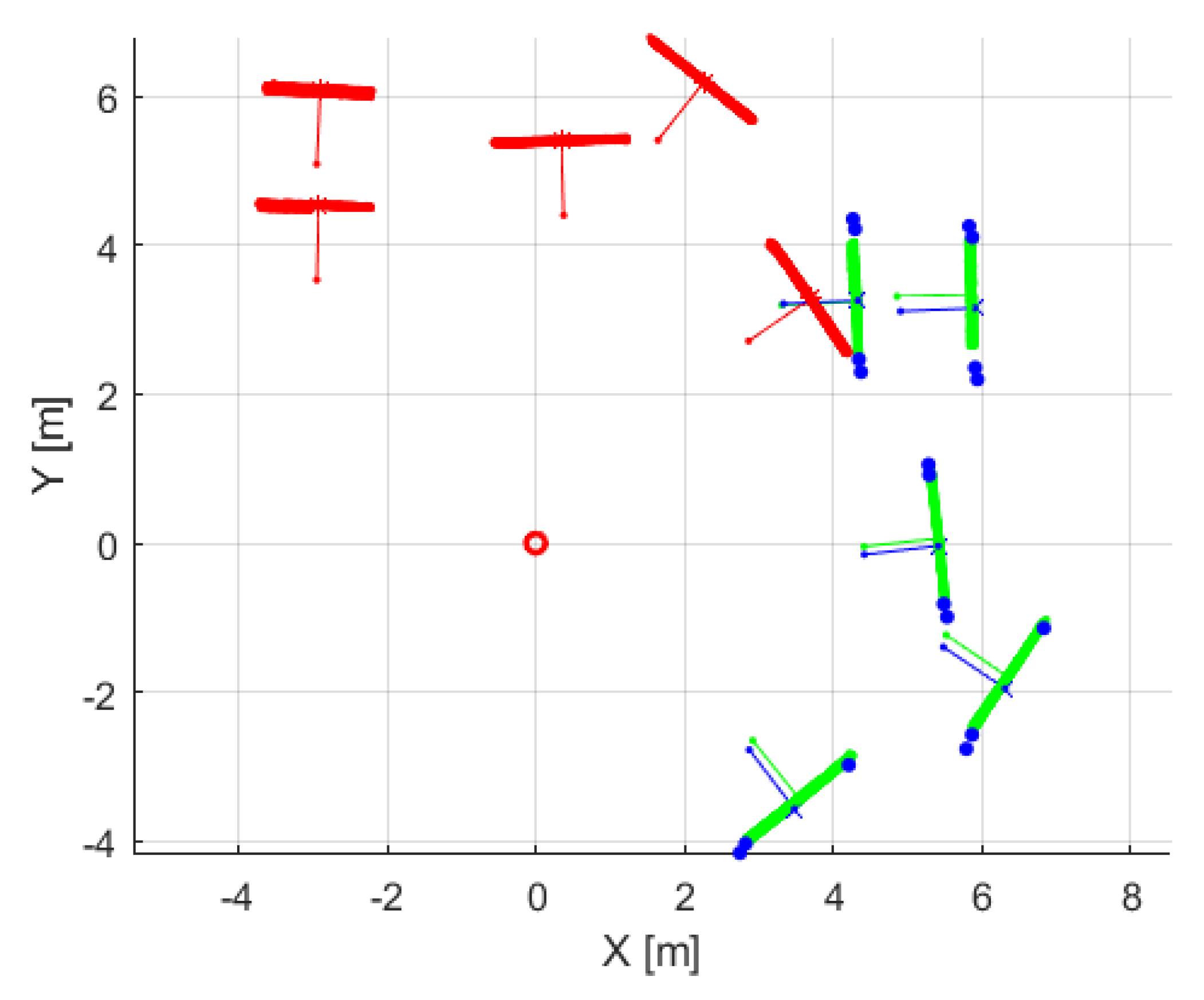
The first step of the data processing is the sensor georeferencing, described in Section 2.3. Figure 10 shows the arrangement for one sensor using the calibration board at five different locations; the points captured by the sensor in the sensor coordinate system are shown in red, and the red lines are the surface norms of the boards calculated from these points. The blue lines are the norms of the boards at the five locations in the global coordinate system; these norms are derived from the board corners (blue dots) measured with a total station. Note that the global coordinate system is connected to the local coordinate system of which origin is the sensor position calculated with GPS. The transformation parameters between the two systems are estimated based on Equation (1). In the Figure 10, the green color depicts the boards after transforming the sensor points into the global frame. The standard deviation of the residuals of the parameter estimation is 0.3°.
Once all individual sensor data were transformed into the global coordinate system, the dynamic content, i.e., the aircraft body, is separated from the static background according to Section 2.3. Three algorithms listed in Table 3 are compared for Test #1. The COG algorithm is a straight-forward model-free object tracking method. In our implementation, the COG points for each scan is calculated as the average (center of gravity) of the object points. Then, the trajectory is derived with, first, smoothing the COG points with a Gaussian filter, and then, resampled with spline interpolation in order for densifying the trajectory points. The second investigated method is the model-based volume minimization introduced in Section 2.6; a 2D CA motion is assumed due to the taxiing scenario in Test #1. The third CT algorithm uses the output of a VM algorithm assuming CV motion as initial reconstruction. Then, the CT algorithm refines this solution by estimating a 2D fourth-degree polynomial motion model. Figure 11 illustrates the points of the airplane body at different times and then the reconstruction by the CT algorithm. Figure 12 presents the reconstructions for the three methods. The quality of the reconstructions can be easily compare by visual assessment. For trajectory solutions, a reference point of the airplane body has to be chosen, and the lowermost point of the front wheel was selected here. Figure 13 presents the trajectories calculated by the three methods.
Landing airplanes were captured from a 33-m object–sensor distance during Test #2. The point density is about 20 points per scan. This is very low point density for the COG algorithm, and thus, the algorithm was not able to produce any acceptable results; subsequently, only the results of the CT algorithm are presented. Figure 14 shows raw airplane points in green, and the reconstruction in blue, and Figure 15 visualizes the reconstructed airplane body in perspective view. Finally, Figure 16 shows the estimated coordinates of a landing aircraft. The red line is the initial VM solution assuming CV motion model. The blue line is the refined CT solution.
5. Discussion
The authors introduced the VM algorithm in an earlier study and used this algorithm assuming 2D constant velocity model [11]. In that study, we showed that the VM outperforms the ICP algorithm based on data captured by a single sensor. The analysis with using GPS installed on the airplane and used as reference showed that the RMSEs (root-mean-square errors) are 0.72 m/s with VM and 5.29 m/s with ICP even at short (10 m) object–sensor distances. The main reason that the ICP tends to fail is that it requires corresponding points between two point clouds; point clouds acquired by the Velodyne scanners have relatively low point density or resolution, especially when the object–sensor distance is large. Consequently, capturing “good” corresponding points is not possible.
While the VM performed well for the CV model in our earlier studies, later it turned out that the VM approach cannot adequately handle more complex motions due to the structure of the objective function at small scale. In our next study, we tried to address this issue of approximating the general motion model by applying the constant velocity model for shorter time periods [12]. This solution performed well, yet it was not robust. This study introduced cube trajectories to improve the motion estimation.
Results have to be compared in terms of accuracy, reliability under various aircraft motions. In the following, two indicators are used for qualitatively assessing and comparing the performance.
- The reconstruction quality is one indicator that can be used to compare the various algorithms and to assess the performance in general. If the reconstruction is good, the aircraft and its details are recognizable, indicating that the derived motion pattern is also close to the actual trajectory. A fuzzy, blurry reconstruction indicates that the estimated motion is not adequate. The reconstructions of the COG, VM-CA and CT algorithms in Figure 15 show that VM and CT outperform COG and CT provides a better reconstruction than VM. The CT reconstruction is fuzzy compared to the reconstruction provided by the CT algorithm. The reason of the underperformance of the COG method is that different body points are backscattered at different epochs, and consequently, the COG does not accurately represent the center of gravity of the airplane body. Clearly, COG tends to fail when the scans contain small number of points from the tracked object. This is also the case for Test #2, when the object sensor distance is around 33 m, and thus, not enough points are captured from the Cessna-size airplanes. In addition, the sensor network is installed on one side of the runway, which means that the sensors capture points from one side of the airplane. This clearly pulls the COG to the direction of that of the sensors. In contrast to COG, the CT is able to provide a fairly good quality reconstruction (see Figure 15), indicating that the algorithm performs well even if the scans contain a small number of points.
- The shape of the trajectory and the velocity profiles can be also used to assess the performance. For instance, in Figure 13 for Test #1, the trajectory derived from COG is not realistic, it is not possible that the airplane could have followed such a curvy trajectory. Note that large tail at the end of the trajectory, which is definitely not feasible motion, is caused by the lack of a sufficient number of captured points. In contrast, the VM-CA and CT results are feasible trajectories. However, it is unclear whether the small “waves” of the CT trajectory is the actual motion of the airplane, or it is the result of overfitting due to fourth-degree motion model. Nevertheless, the largest difference between the two trajectories is about 10 cm, which is within the error envelope detected earlier in our previous studies. The trajectory along the X, Y, and Z directions for Test #2 can be seen in Figure 16. This figure shows the decreasing altitude (see the Z component) as expected for landing aircraft. Also note that the CV model depicted with red in the Figure 16 is a line; however, it is very unlikely that this motion component behaves such a way. The CT solution depicted with blue follows a more realistic trajectory.
Unfortunately, reference solution, for instance, from GPS, is not available for the quantitative analysis of the methods. However, the residuals from the CT algorithm can describe the “internal” accuracy between the measured cube velocities and the underlying motion model. The average and standard deviation of the absolute residuals from the CT algorithm are presented in Table 4.
The statistics of the average absolute residuals (0.06–0.69 m/s) are similar to those we experienced earlier for simpler motions. The X velocity errors are dominant for both cases, but significantly larger than the Y component in the case of the Taxiing data; note that the X axis is the direction of landing and taxiing. The accuracies of the Y and Z components are similar. The standard deviation is also relatively low (0.08–0.17 m). Note that the residuals are velocities, and do not describe the positioning accuracy directly. The sampling frequency of the sensors is 10 Hz, and thus, the positioning error is supposed to be around one to seven centimeters based on these velocity residuals.
Limitations and Possible Applications
The prototype system allows for real-time tracking of aircraft during taxiing, landing or takeoffs. Figure 17 shows an example of a user interface, where a landing aircraft is tracked, and the demonstration system provides the velocity, altitude and position including the error envelopes along with video feedback. Currently, the main limitation of the developed system is the small observation space, which is an affordability issue. To cover larger sections along runways and taxiways would require large number of sensors, which would increase the price of the system and the operation costs. However, mobile LiDAR scanners, such as Velodyne sensors, are expected to become cheaper in the coming years due to the increasing needs for mass production boosted by the autonomous car industry. There are other applications where the proposed system is applicable at airports. For instance, LiDAR might offer tracking solution in night or bad visibility conditions, when optical sensing is compromised. Obviously, LiDAR will fail in extreme weather conditions, such as heavy raining or snowing. With improving resolution and coverage, aircraft types can be the detected and models identified. Figure 18 shows the reconstruction of a Cessna and a Learjet, where details seem to adequate for aircraft model identification. Note that the scale is preserved in LiDAR data, making object identification easier. Clearly, machine learning or other algorithms can be developed to identify the types of the incoming airplanes captured by the LiDAR sensor network [9]. In addition, LiDAR as remote sensing technology, can also be used for monitoring the surroundings to detect and identify hazardous objects to improve the safety of apron operations (see [9,10]).
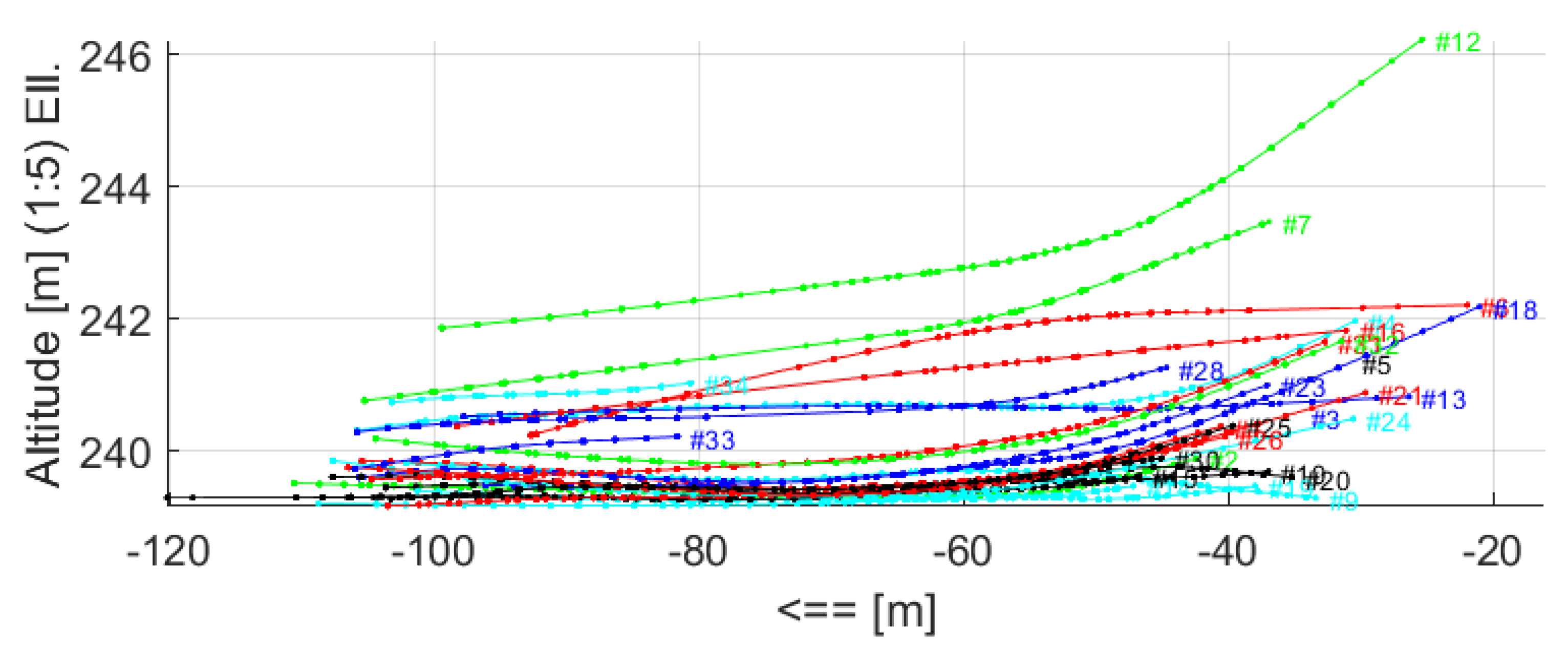
Besides the possible applications presented above, the original intent of this effort was to develop a LiDAR-based prototype system to demonstrate the feasibility that airplanes can be identified and tracked in airport environment without any cooperation from the aircraft. Note that aircraft navigation systems provide this information to the crew, but this data is not shared by airport authorities. Using remote technology provides non-cooperative alternative for collecting huge amount of motion parameters that can improve airport safety through helping understand and assess the risk of the pilot’s driving patterns on the runways and taxiways (e.g., centerline deviation, wingspan separation). This information can be used in aircraft and airport planning, e.g., whether the airport meets the standardized criteria or providing data for modification of airport standards and pilot education. To develop adequate risk models for taxiing behavior, Chou et al. used positioning gauges to obtain data at the Chiang-Kai-Shek International Airport [24]. Another study from FAA/Boeing investigated the 747s’ centerline deviations at JFK and ANC airports [25,26,27]. They used laser diodes at two locations to measure the location of the nose and main gears. These approaches allow only for accurate on-ground aircraft tracking as opposed to the LiDAR-based tracking system that is also capable of tracking during landing or takeoffs with high accuracy. Figure 19 shows the trajectories of all landing airplanes during Test #2.
6. Conclusions
The paper discussed the feasibility of using a LiDAR sensor network to accurately track taxiing and landing aircraft. The used sensors—the Velodyne VLP-16 and HDL-32E—provide high sampling rates to capture an aircraft during taxiing or landing with relatively high speed; however, the captured point clouds are sparse. The main reason for the small number of LiDAR points captured from the aircraft body is the large, ~20–30 m object–sensor distance. This issue is addressed in the paper by presenting two novel model-based tracking algorithms. First, the VM algorithm is developed to find the parameters of a simple motion model, such as CV or CA, with minimizing the reconstruction volume. Then, the CT algorithm uses these reconstructions, as an initial solution, to find the parameters of the general motion model. The proposed method outperformed the COG method, and could achieve one- to seven-centimeter tracking accuracy. The VM and CT algorithms perform really well on the acquired datasets. However, the dynamics of the motion in the presented examples is low, and therefore, it is required to assess the performance for more complex trajectories. Currently, sharp turning scenarios may not be handled with the presented algorithm. In the future, we plan to extend the algorithms considering these motions in the model to be able to handle more complex maneuvers. The developed approach might be also used in other applications outside of the aviation domain, such as tracking vehicle traffic, etc.
Supplementary Materials
C++ code with Matlab interface and sample data are available online at https://github.com/zkoppanyi/cas.
Acknowledgments
The authors would like to thank the Ohio State University Airport as the test site for this research and the Federal Aviation Administration who supported this work through the Center of Excellence for General Aviation, known as PEGASAS, the Partnership to Enhance General Aviation Safety Accessibility, and Sustainability. Although the FAA has sponsored this project, it neither endorses nor rejects the findings of this research.
Author Contributions
C. T. conceived the experiment. Z. K. conceived the sensor georeferencing. Z. K. and C. T. designed and performed the experiment. Z. K. conducted the data processing, analysis, and developed the algorithms. Z. K. and C. T. wrote the paper.
Conflicts of Interest
The authors declare no conflict of interest.
Appendix A
This appendix explains some basic definitions used throughout the paper. A point captured by a LiDAR sensor is given with its X, Y and Z coordinates as well as the time when it was captured, i.e., , where is the set of points. A set is a point cloud, where is the set of point clouds and is the power set of . Consequently, contains no or many points. A scan is a point cloud collected by the sensor when it makes a complete 360° scan starting from 0°. Note that the times of the points in a scan might be different but has to be within the sampling time; this is the time to make a full 360° scan. The reverse direction is not valid, points within the sampling time might not correspond to the same scan. The data collected by the sensor can be split into scans, and consequently, the collected data is a series of consecutive scans. The reconstruction or reconstructed point cloud is a point cloud that contains several transformed scans. In the paper, the scans are typically transformed based on a chosen motion model, resulting in a reconstruction.
Appendix B
The applied motion models are very simple, yet his appendix summarizes these basic formulas for the sake of completeness. The general 2D motion considering a pointwise particle can be described as time variable polynomial functions:
where, and are the parameters of the motion. This model can be extended with the Z coordinate in the case of 3D motions, such that
The model can be simplified that results in the constant acceleration (CA) model for curvilinear motions:
where are the starting position, are the velocities, are the accelerations along X, Y, Z directions, and is the time. Finally, the 3D constant velocity (CV) model is
A point from the cloud can be transformed back to zero time. For instance, for the general motion model, with knowing the , motion parameters, the transformation takes the following form:
Applying these equations for all captured points results in a point cloud called reconstructed point cloud or reconstruction.
Appendix C
Algorithm A1 presents the steps for the simulated annealing method to solve volume minimization defined in Equation (2).
| Algorithm A1 Simulated annealing algorithm for volume minimization | |
|
References
- Toth, C.; Jóźków, G. Remote sensing platforms and sensors: A survey. ISPRS J. Photogramm. Remote Sens. 2016, 115, 22–36. [Google Scholar] [CrossRef]
- Navarro-Serment, L.E.; Mertz, C.; Hebert, M. Pedestrian Detection and Tracking Using Three-Dimensional LADAR Data. In Field and Service Robotics; Springer Tracts in Advanced Robotics; Springer: Berlin, Germany, 2010; pp. 103–112. ISBN 978-3-642-13407-4. [Google Scholar]
- Cui, J.; Zha, H.; Zhao, H.; Shibasaki, R. Laser-based detection and tracking of multiple people in crowds. Comput. Vis. Image Underst. 2007, 106, 300–312. [Google Scholar] [CrossRef]
- Sato, S.; Hashimoto, M.; Takita, M.; Takagi, K.; Ogawa, T. Multilayer lidar-based pedestrian tracking in urban environments. In Proceedings of the 2010 IEEE Intelligent Vehicles Symposium, San Diego, CA, USA, 21–24 June 2010; pp. 849–854. [Google Scholar]
- Tarko, P.; Ariyur, K.B.; Romero, M.A.; Bandaru, V.K.; Liu, C. Stationary LiDAR for Traffic and Safety Applications–Vehicles Interpretation and Tracking; USDOT: Washington, DC, USA, 2014.
- Börcs, A.; Nagy, B.; Benedek, C. On board 3D object perception in dynamic urban scenes. In Proceedings of the 2013 IEEE 4th International Conference on Cognitive Infocommunications (CogInfoCom), Budapest, Hungary, 2–5 December 2013; pp. 515–520. [Google Scholar]
- Toth, C.K.; Grejner-Brzezinska, D. Extracting dynamic spatial data from airborne imaging sensors to support traffic flow estimation. ISPRS J. Photogramm. Remote Sens. 2006, 61, 137–148. [Google Scholar] [CrossRef]
- Statistical Summary of Commercial Jet Airplane Accidents Worldwide Operations. Available online: http://www.boeing.com/resources/boeingdotcom/company/about_bca/pdf/statsum.pdf (accessed on 16 December 2017).
- Mund, J.; Frank, M.; Dieke-Meier, F.; Fricke, H.; Meyer, L.; Rother, C. Introducing LiDAR Point Cloud-based Object Classification for Safer Apron Operations. In Proceedings of the International Symposium on Enhanced Solutions for Aircraft and Vehicle Surveillance Applications, Berlin, Germany, 7–8 April 2016. [Google Scholar]
- Mund, J.; Zouhar, A.; Meyer, L.; Fricke, H.; Rother, C. Performance Evaluation of LiDAR Point Clouds towards Automated FOD Detection on Airport Aprons. In Proceedings of the 5th International Conference on Application and Theory of Automation in Command and Control Systems, Toulouse, France, 30 September–2 October 2015. [Google Scholar]
- Koppanyi, Z.; Toth, C. Estimating Aircraft Heading based on Laserscanner Derived Point Clouds. In Proceedings of the ISPRS Annals of the Photogrammetry, Remote Sensing and Spatial Information Sciences, Munich, Germany, 25–27 March 2015; Volume II-3/W4, pp. 95–102. [Google Scholar]
- Toth, C.; Jozkow, G.; Koppanyi, Z.; Young, S.; Grejner-Brzezinska, D. Monitoring Aircraft Motion at Airports by LiDAR. In Proceedings of the ISPRS Annals of the Photogrammetry, Remote Sensing and Spatial Information Sciences, Prague, Czech Republic, 12–19 July 2016; Volume III-1, pp. 159–165. [Google Scholar]
- VLP-16 Manual. Available online: http://velodynelidar.com/vlp-16.html (accessed on 15 December 2017).
- HDL-32E Manual. Available online: http://velodynelidar.com/hdl-32e.html (accessed on 15 December 2017).
- Wang, D.Z.; Posner, I.; Newman, P. Model-free Detection and Tracking of Dynamic Objects with 2D Lidar. Int. J. Robot. Res. 2015, 34, 1039–1063. [Google Scholar] [CrossRef]
- Pomerleau, F.; Colas, F.; Siegwart, R. A Review of Point Cloud Registration Algorithms for Mobile Robotics. Found. Trends Robot. 2015, 4, 1–104. [Google Scholar] [CrossRef]
- Moosmann, F.; Stiller, C. Joint self-localization and tracking of generic objects in 3D range data. In Proceedings of the 2013 IEEE International Conference on Robotics and Automation, Karlsruhe, Germany, 6–10 May 2013; pp. 1146–1152. [Google Scholar]
- Dewan, A.; Caselitz, T.; Tipaldi, G.D.; Burgard, W. Motion-based detection and tracking in 3D LiDAR scans. In Proceedings of the 2016 IEEE International Conference on Robotics and Automation (ICRA), Stockholm, Sweden, 16–21 May 2016; pp. 4508–4513. [Google Scholar]
- Kaestner, R.; Maye, J.; Pilat, Y.; Siegwart, R. Generative object detection and tracking in 3D range data. In Proceedings of the 2012 IEEE International Conference on Robotics and Automation, Saint Paul, MN, USA, 14–18 May 2012; pp. 3075–3081. [Google Scholar]
- Dierenbach, K.; Jozkow, G.; Koppanyi, Z.; Toth, C. Supporting Feature Extraction Performance Validation by Simulated Point Cloud. In Proceedings of the ASPRS 2015 Annual Conference, Tampa, FL, USA, 4–8 May 2015. [Google Scholar]
- Saez, J.M.; Escolano, F. Entropy Minimization SLAM Using Stereo Vision. In Proceedings of the 2005 IEEE International Conference on Robotics and Automation, Barcelona, Spain, 18–22 April 2005; pp. 36–43. [Google Scholar]
- Saez, J.M.; Hogue, A.; Escolano, F.; Jenkin, M. Underwater 3D SLAM through entropy minimization. In Proceedings of the 2006 IEEE International Conference on Robotics and Automation, Orlando, FL, USA, 15–19 May 2006; pp. 3562–3567. [Google Scholar]
- Aarts, E.; Korst, J.; Michiels, W. Simulated Annealing. In Search Methodologies; Springer: Boston, MA, USA, 2005; pp. 187–210. ISBN 978-0-387-23460-1. [Google Scholar]
- Chou, C.P.; Cheng, H.J. Aircraft Taxiing Pattern in Chiang Kai-Shek International Airport. In Airfield and Highway Pavement: Meeting Today’s Challenges with Emerging Technologies, Proceedings of the Airfield and Highway Pavements Specialty Conference, Atlanta, GA, USA, 30 April–3 May 2006; American Society of Civil Engineers: Reston, VA, USA, 2016. [Google Scholar] [CrossRef]
- Sholz, F. Statistical Extreme Value Analysis of ANC Taxiway Centerline Deviation for 747 Aircraft; FAA/Boeing Cooperative Research and Development Agreement; Federal Aviation Administration: Washington, DC, USA, 2003.
- Sholz, F. Statistical Extreme Value Analysis of JFK Taxiway Centerline Deviation for 747 Aircraft; FAA/Boeing Cooperative Research and Development Agreement; Federal Aviation Administration: Washington, DC, USA, 2003.
- Sholz, F. Statistical Extreme Value Concerning Risk of Wingtip to Wingtip or Fixed Object Collision for Taxiing Large Aircraft; Federal Aviation Administration: Washington, DC, USA, 2005.
Figure 1.
Sensor system overview: (a) horizontally and (b) vertically aligned VLP-16 sensor, (c) components of the demonstration sensor network, and (d) sensor coverage.
Figure 1.
Sensor system overview: (a) horizontally and (b) vertically aligned VLP-16 sensor, (c) components of the demonstration sensor network, and (d) sensor coverage.

Figure 2.
Sensor georeferencing: calibration board with surveying prism (upper left corner) measured with total station and sensor station.
Figure 2.
Sensor georeferencing: calibration board with surveying prism (upper left corner) measured with total station and sensor station.

Figure 3.
Top-down views from an airplane captured at different times by the sensor network. The two subfigures illustrate the point densities at different object–sensor distances: color differentiates scans: (a) at 23 m object–sensor distance, the average number of points per scan is 130 (26 per sensor), and (b) at 33 m object–sensor distance, the average number of points per scan is 20 (4 points from each sensor).

Figure 4.
The idea of volume minimization: figures show reconstructions (with red dots) assuming a constant velocity (CV) model with different velocities; green points are the raw data, black rectangles show the occupied cubes, and titles show velocities and number of cubes obtained.
Figure 4.
The idea of volume minimization: figures show reconstructions (with red dots) assuming a constant velocity (CV) model with different velocities; green points are the raw data, black rectangles show the occupied cubes, and titles show velocities and number of cubes obtained.
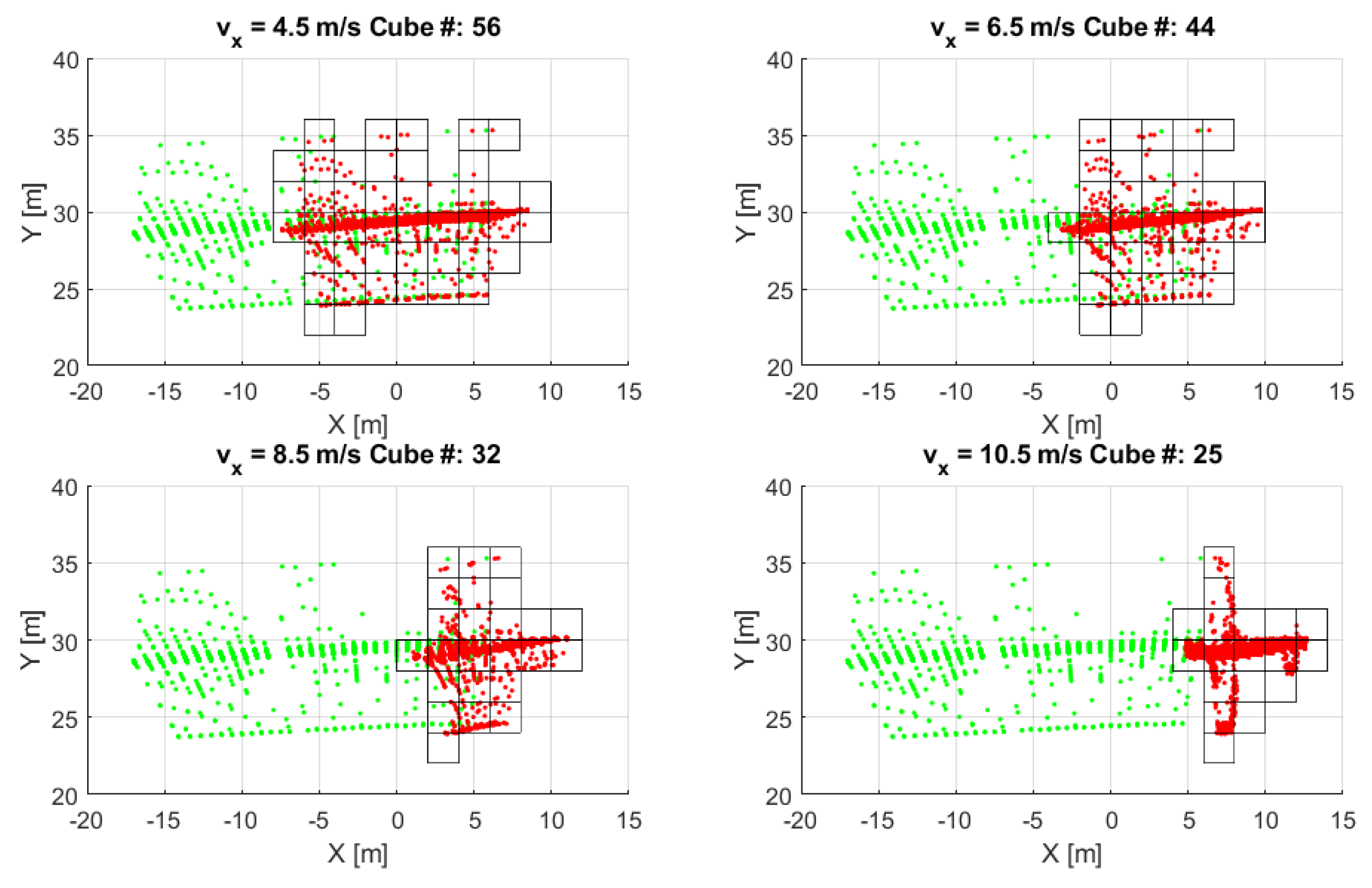
Figure 5.
Measuring the volume of the reconstruction: the space is decimated with cubes, and the volume is represented by the number of cubes occupied by the reconstruction.
Figure 5.
Measuring the volume of the reconstruction: the space is decimated with cubes, and the volume is represented by the number of cubes occupied by the reconstruction.

Figure 6.
Illustration of the problem space for CV motion model at various scales: (a) large, (b) medium, and (c) small scale.
Figure 6.
Illustration of the problem space for CV motion model at various scales: (a) large, (b) medium, and (c) small scale.

Figure 7.
Illustration of the cube trajectory (CT) algorithm: the initial reconstruction (red dots) is calculated from the data (blue dots), then this reconstruction is decimated into cubes, and then the trajectories (black lines) of all cubes are determined based on the points in the cubes.
Figure 7.
Illustration of the cube trajectory (CT) algorithm: the initial reconstruction (red dots) is calculated from the data (blue dots), then this reconstruction is decimated into cubes, and then the trajectories (black lines) of all cubes are determined based on the points in the cubes.

Figure 8.
Time–velocity graph of cubes from curvy linear motion: the cube velocities along the X and Y directions are depicted with blue and red dots, respectively; in this example, a constant acceleration (CA) motion model is used, thus the parameters a line are estimated with regression.
Figure 8.
Time–velocity graph of cubes from curvy linear motion: the cube velocities along the X and Y directions are depicted with blue and red dots, respectively; in this example, a constant acceleration (CA) motion model is used, thus the parameters a line are estimated with regression.

Figure 9.
Test sensor configurations: (a) Test #1 sensor network (taxiing), and (b) Test #2 sensor network configuration (landing).
Figure 9.
Test sensor configurations: (a) Test #1 sensor network (taxiing), and (b) Test #2 sensor network configuration (landing).


Figure 10.
Sensor georeferencing: points from the calibration board in the sensor coordinate system depicted with red, the norm of the board surface is shown with red lines, blue dots are the board corners measured with total station, the blue lines are the norms of the board surface in the global coordinate system, green points depict the points after transforming the board points from the sensor to the global coordinate system, and the red circle marks the sensor position.

Figure 11.
Green points mark the raw dataset captured from a taxiing aircraft during Test #1, and red points show the reconstructed airplane body using the CT method.
Figure 11.
Green points mark the raw dataset captured from a taxiing aircraft during Test #1, and red points show the reconstructed airplane body using the CT method.
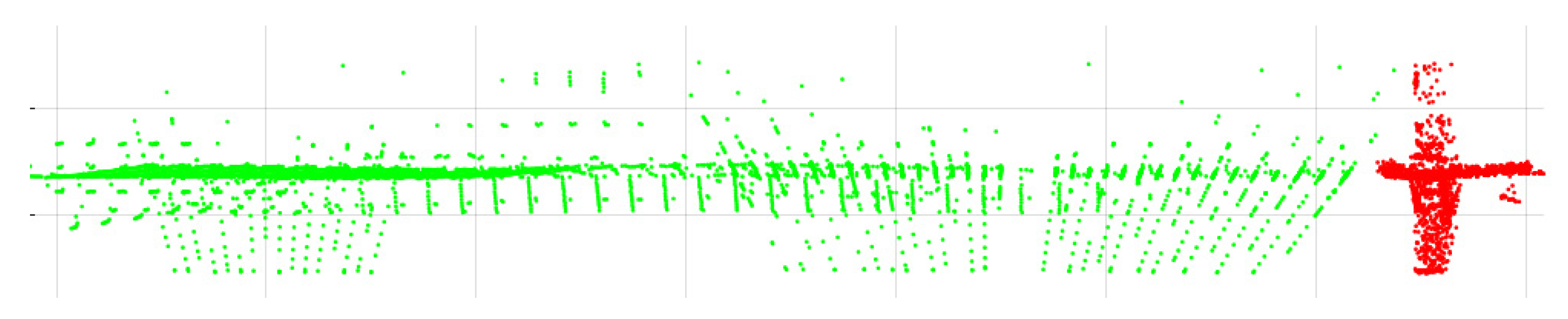
Figure 12.
Reconstructions by the three algorithms for Test #1 from data presented in Figure 11: (a) center of gravity (COG), (b) volume minimization with CA motion model (VM-CA), and (c) cube trajectories (CT).
Figure 12.
Reconstructions by the three algorithms for Test #1 from data presented in Figure 11: (a) center of gravity (COG), (b) volume minimization with CA motion model (VM-CA), and (c) cube trajectories (CT).

Figure 13.
Trajectory solutions for the three methods.
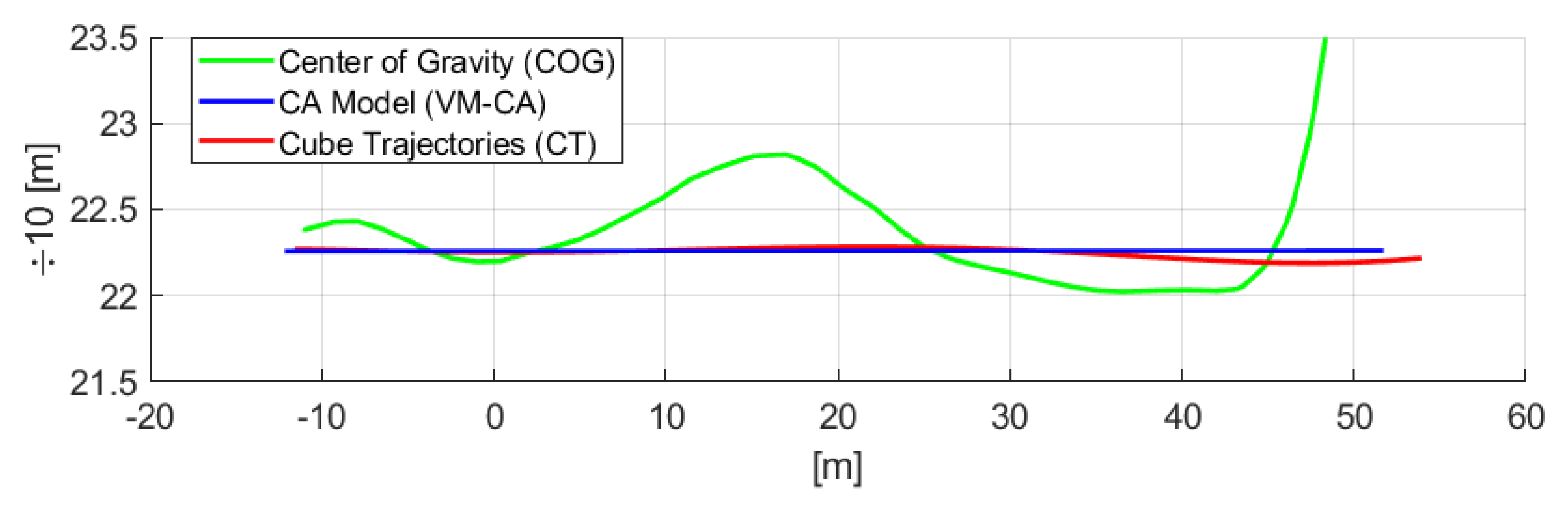
Figure 14.
Reconstruction from sparse point clouds (average point density is 36/scans or 7.2 points/scan/sensor), using the CT algorithm for a landing Cessna airplane during Test #2: the captured airplane points are shown in green, the reconstruction is in blue.
Figure 14.
Reconstruction from sparse point clouds (average point density is 36/scans or 7.2 points/scan/sensor), using the CT algorithm for a landing Cessna airplane during Test #2: the captured airplane points are shown in green, the reconstruction is in blue.
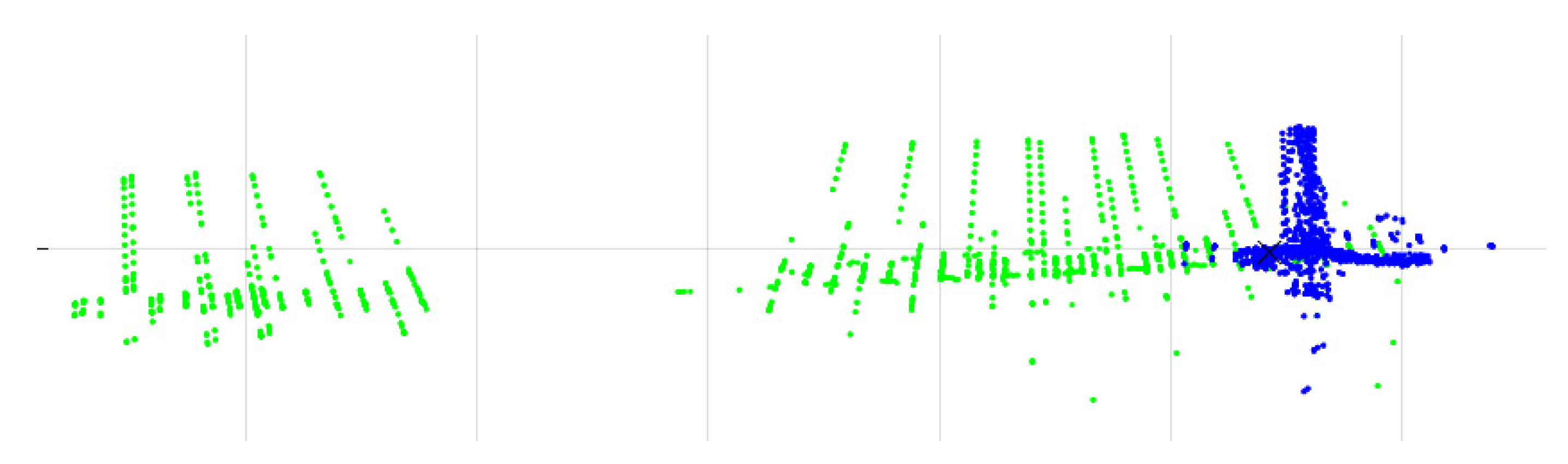
Figure 15.
Reconstruction from sparse point clouds (total number of points is 4320) from data presented in Figure 14: the shape of the plane including the wings, tails are recognizable.
Figure 15.
Reconstruction from sparse point clouds (total number of points is 4320) from data presented in Figure 14: the shape of the plane including the wings, tails are recognizable.
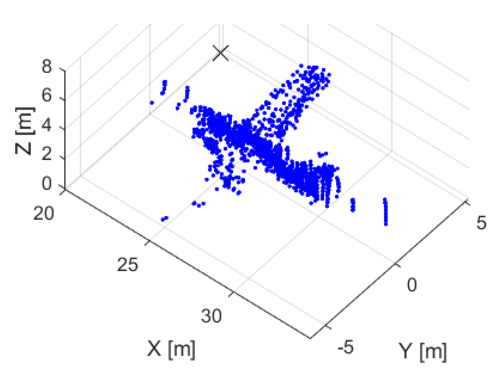
Figure 16.
Estimated coordinates of a landing Cessna airplane using VM-CV (red) and CT (blue) algorithms for the X, Y, and Z directions; X direction is along the centerline of the runway.
Figure 16.
Estimated coordinates of a landing Cessna airplane using VM-CV (red) and CT (blue) algorithms for the X, Y, and Z directions; X direction is along the centerline of the runway.
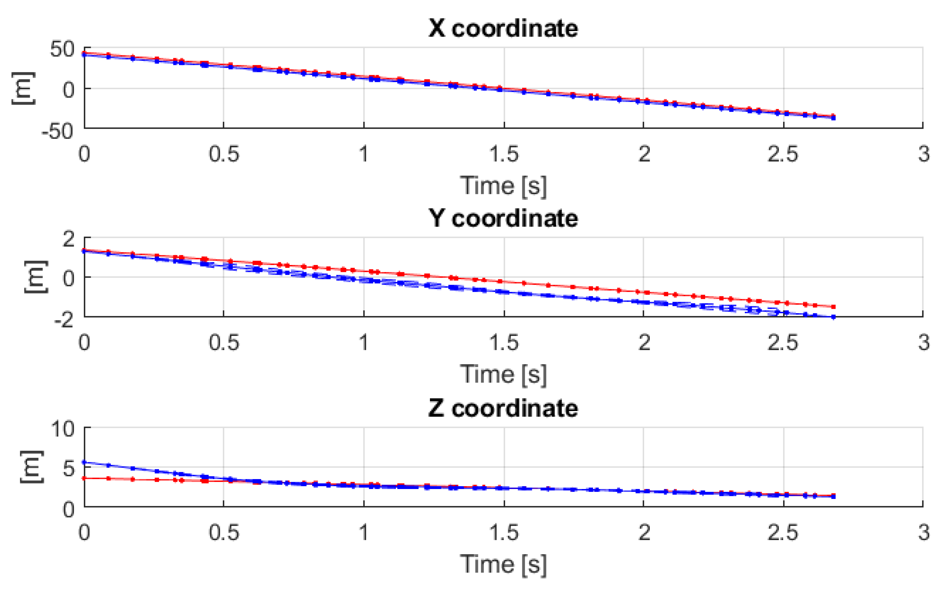
Figure 17.
Aircraft tracking: (a) current video frame, (b) altitude profile with blue dashed line showing the error envelope in cm, red line is the runway surface, and (c) 2D trajectory.
Figure 17.
Aircraft tracking: (a) current video frame, (b) altitude profile with blue dashed line showing the error envelope in cm, red line is the runway surface, and (c) 2D trajectory.
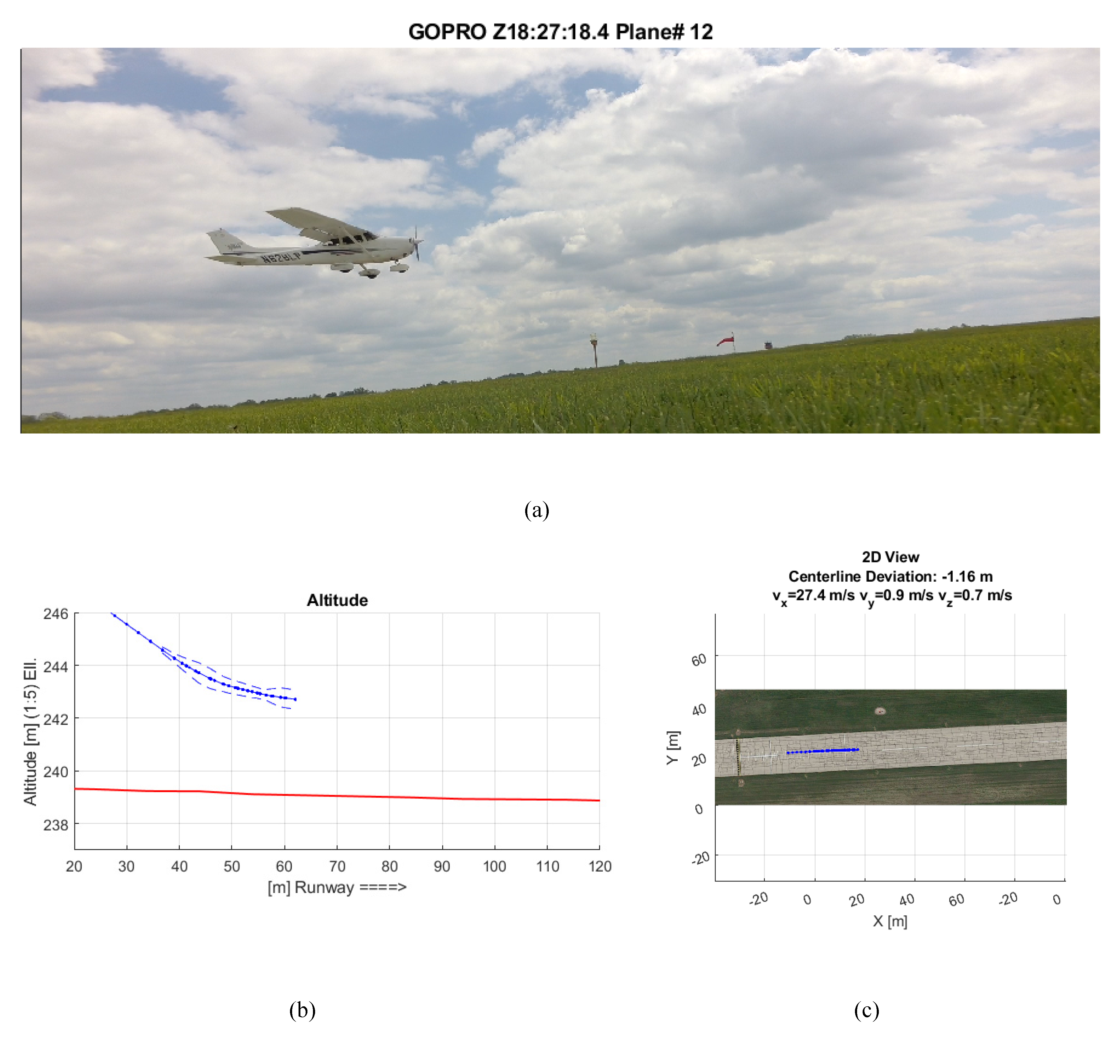
Figure 18.
Reconstruction of different aircraft types, (a) Cessna and (b) Learjet.

Figure 19.
Altitude profiles of 29 landing airplanes from Test #2.


Table 1.
Motion models used in this study; more details can be found in Appendix B.
Table 1.
Motion models used in this study; more details can be found in Appendix B.
| Constant Velocity | Constant Acceleration | General or Polynomial |
|---|---|---|
Table 2.
Overview of the field tests (* projected to the runway centerline).
| Test Case | Goal | Sensors | Field of View * | Object–Sensor Distance | |
|---|---|---|---|---|---|
| #1 | Taxiing | 2D performance at taxiing | 3 vertical VLP-16s, 1 horizontal HDL-32E | 70 m | 20 m |
| #2 | Landing | 3D performance at landing | 4 vertical VLP-16s, 1 horizontal HDL-32E | 100 m | 33 m |
Table 3.
Investigated algorithms for Test #1.
| Method | Parameters |
|---|---|
| Center of Gravity (COG) | The COG points are filtered with a Gaussian kernel and resampled with spline interpolation |
| Volume Minimization with CA motion model | Cube size is 1 m, other parameters are presented in Section 2.6. |
| Refinement with Cube Trajectories | Initial reconstruction using a CV model and SA, motion model is fourth-degree polynomial |
Table 4.
Quantitative statistics of the CT method.
| Test | Average of the Absolute Residuals | Standard Deviation of the Absolute Residuals | ||||
|---|---|---|---|---|---|---|
| X (m/s) | Y (m/s) | Z (m/s) | X (m/s) | Y (m/s) | Z (m/s) | |
| #1 Taxiing | 0.69 | 0.06 | - | 0.44 | 0.00 | - |
| #2 Landing | 0.67 | 0.44 | 0.51 | 0.17 | 0.08 | 0.11 |
© 2018 by the authors. Licensee MDPI, Basel, Switzerland. This article is an open access article distributed under the terms and conditions of the Creative Commons Attribution (CC BY) license (http://creativecommons.org/licenses/by/4.0/).
Share and Cite
MDPI and ACS Style
Koppanyi, Z.; Toth, C.K. Object Tracking with LiDAR: Monitoring Taxiing and Landing Aircraft. Appl. Sci. 2018, 8, 234. https://doi.org/10.3390/app8020234
AMA Style
Koppanyi Z, Toth CK. Object Tracking with LiDAR: Monitoring Taxiing and Landing Aircraft. Applied Sciences. 2018; 8(2):234. https://doi.org/10.3390/app8020234
Chicago/Turabian StyleKoppanyi, Zoltan, and Charles K. Toth. 2018. "Object Tracking with LiDAR: Monitoring Taxiing and Landing Aircraft" Applied Sciences 8, no. 2: 234. https://doi.org/10.3390/app8020234
Note that from the first issue of 2016, this journal uses article numbers instead of page numbers. See further details here.