Improvement to the Huff Curve for Design Storms and Urban Flooding Simulations in Guangzhou, China


1
Center of Integrated Geographic Information Analysis, School of Geography and Planning, and Guangdong Key Laboratory for Urbanization and Geo-simulation, Sun Yat-sen University, Guangzhou 510275, China
2
Department of Geography, University of Cincinnati, Cincinnati, OH 45221, USA
*
Authors to whom correspondence should be addressed.
Water 2017, 9(6), 411; https://doi.org/10.3390/w9060411
Submission received: 24 March 2017
/
Revised: 9 May 2017
/
Accepted: 5 June 2017
/
Published: 8 June 2017
(This article belongs to the Special Issue Applications of Remote Sensing/GIS in Water Resources and Flooding Risk Managements)
Abstract
:The storm hyetograph is critical in drainage design since it determines the peak flooding volume in a catchment and the corresponding drainage capacity demand for a return period. This study firstly compares the common design storms such as the Chicago, Huff, and Triangular curves employed to represent the storm hyetographs in the metropolitan area of Guangzhou using minute-interval rainfall data during 2008–2012. These common design storms cannot satisfactorily represent the storm hyetographs in sub-tropic areas of Guangzhou. The normalized time of peak rainfall is at 33 ± 5% for all storms in the Tianhe and Panyu districts, and most storms (84%) are in the 1st and 2nd quartiles. The Huff curves are further improved by separately describing the rising and falling limbs instead of classifying all storms into four quartiles. The optimal time intervals are 1–5 min for deriving a practical urban design storm, especially for short-duration and intense storms in Guangzhou. Compared to the 71 observed storm hyetographs, the Improved Huff curves have smaller RMSE and higher NSE values (6.43, 0.66) than those of the original Huff (6.62, 0.63), Triangular (7.38, 0.55), and Chicago (7.57, 0.54) curves. The mean relative difference of peak flooding volume simulated with SWMM using the Improved Huff curve as the input is only 2%, −6%, and 8% of those simulated by observed rainfall at the three catchments, respectively. In contrast, those simulated by the original Huff (−12%, −43%, −16%), Triangular (−22%, −62%, −38%), and Chicago curves (−17%, −19%, −21%) are much smaller and greatly underestimate the peak flooding volume. The Improved Huff curve has great potential in storm water management such as flooding risk mapping and drainage facility design, after further validation.
1. Introduction
The storm hyetograph is crucial not only for urban storm water management, but also for the catchment hydrology in general [1,2,3,4]. Given a total rainfall depth and duration for a certain return period, the storm hyetograph determines the peak flow/time and the drainage capability demand in a catchment [5,6]. Therefore, the accurate representation of the storm hyetograph is significant for designing suitable drainage facilities and reducing the flooding risk in an urban catchment.
Urban flooding events have frequently occurred and increased in many cities worldwide in recent years in the context of global warming [7,8,9,10,11]. China faces even more severe challenges in urban flooding due to its dramatic urbanization and relatively poor storm water management [12]. In order to mitigate the impacts of urban flooding, the Chinese government has issued a series of regulations on urban storm water management [13,14,15]. Several design storms are recommended for drainage facility design in those regulations, including the Triangular curve [16], the Chicago curve [17], and the Soil Conservation Service (SCS) curve [18].
The Triangular curve was developed by Yen & Chow [16] for drainage design in a small catchment and is widely used in natural watersheds and small urban catchments [19,20]. It is a one-parameter model that is estimated by preserving the first moment of the rainfall depth [19]. The Chicago curve is constructed by fitting the equations of the intensity-duration-frequency curves given the total rainfall depth and duration for a return period [17,18,19,20,21]. It is often applied in sewer and flooding drainage design [22,23]. The SCS curve is a dimensionless hyetograph/hydrograph with a single parameter [24]. It was originally developed for designing safe water storage facilities in agricultural applications and has been widely applied in various situations, especially for long duration storm events of 6, 12, 24 h, and even longer [4,25,26,27].
The Huff curve is another popular design hyetograph for characterizing the temporal distributions of rainfall depth in an area [19]. Like the SCS curve, it is also a dimensionless cumulative hyetograph with specified probabilities of occurrence [28] and is widely utilized as a design storm, downscaling analysis of rainfall depth data, and inputs to rainfall-runoff models for drainage design [5,29]. In practice, historic storm data are first classified into four quartiles according to the normalized time of peak rainfall, and a series of Huff curves are then developed at different probabilities within each quartile [29].
The above design storm curves are derived for the entire storms using historic storm data with hourly rainfall accumulation in most cases, except for the Chicago curve. The time of peak rainfall has a critical influence on the classification of the hyetograph [30]. Separating a storm into the rising and falling limbs could better represent the rainfall hyetograph [31]. The Chicago curve uses two formulas to represent the rising and falling limbs, where the rainfall intensity exponentially decreases on both sides of the peak rainfall [32].
Most storms are less than three hours in the Guangzhou Metropolitan areas in South China, identified according to the criteria reported in the following Section 3.1. The partial reason for this frequent flooding is that the pipe system underestimates the peak runoff, which is simulated by using design storms like Chicago and Triangular curves for a given return period. Those design storms are usually derived from hourly rainfall data and thus underestimate the rainfall intensity. As a result of this, they do not satisfactorily represent the real storm hyetograph.
Therefore, the primary objective of this study is to develop a suitable storm hyetograph by improving the Huff model through studying the rising and falling limbs separately based on minute-interval rainfall depth data in the Guangzhou metropolitan areas. A secondary objective is to investigate the sensitivity of the design storm to time intervals of rainfall depth and to offer a suggestion for selecting optimal time intervals of rainfall depth data with urban design storm research. The Improved Huff curve is then validated and compared to the Huff curve, Triangular curve, and Chicago curve by using in situ measurements of storm events and by applying for flooding volume simulation as inputs to the Storm Water Management Model (SWMM) in three small urban catchments.
2. Study Area and Data
2.1. Study Area
The study area is located in the Guangzhou Metropolitan areas in South China (Figure 1). It has a sub-tropic climate controlled by the East Asian Monsoon, more specifically the South China Sea Monsoon. It has warm and wet summers and dry winters, with a mean annual air temperature of 22 °C and annual precipitation of 1700 mm [33]. Over 80% of the annual precipitation falls during the rainy season from April to September [12,34]. This area is well known for its dense interlocking river network and has gone through dramatic urbanization over the past 20 years; the impervious land changed from 12,998 ha in 1990 to 59,911 ha in 2009 [35,36]. In the Tianhe (Site/Rain gauge 2) and Panyu (Site/Rain gauges 1, 3–6) Districts, the imperious land ratio (based on Landsat images) increased from 16% to 71% and from 2% to 40% from 1990 to 2013, respectively. However, most (83%) of the drainage pipes adopted the design standards for storms of a one-year return period, and only 9% of the pipes adopted these for a two-year return period [37]. It is a very low return period. In many countries, a 25-year return period is adopted. Hence, the streets in the city of Guangzhou were frequently inundated.
2.2. Rainfall Depth Data
This study uses two types of rainfall data from six automatic gauges. The first type is from national standard meteorological sites (Sites 1 and 2) of China, where rainfall depth data are automatically recorded at one-minute intervals with a precision of 0.1 mm. Site 2 is within the downtown area of the Tianhe District, whereas Site 1 is in the Panyu District, a sub-urban area. The two sites are 25 km apart. Five-year rainfall data from 2008 to 2012 are obtained to develop and validate the coefficients of the design storms at Sites 2 and 1, respectively. The other four sites (Sites 3–6) were set up at the Panyu District in the summer of 2014 by our research team. Rainfall data are recorded at one-minute intervals with a precision of 1 mm. Meanwhile, an electronic water depth meter was also set up to record the street water depth at Site 4 (Node 503), where flooding inundation has occurred several times each year recently. The storm rainfall and water depth data recorded at Site 4/Node503 is used to optimize the SWMM model and validate the design storms.
3. Methodology
The rainfall data at Site 2 are used to develop the design storms, including the Huff curve, Improved Huff curve, and the Triangular curve. The storm data at Site 1 and Sites 3–6 are used to validate the design storms. These design storms are further applied as inputs to the SWMM model to simulate the flooding volume, which is compared with that from in situ measurements at Node 503. The detailed procedure and methods are arranged below.
3.1. Storm Events
In this study, storm events are identified based on the following criteria: (a) rainfall duration > 20 min [31]; (b) rainfall depth in a one-hour moving window > 20 mm [13]; (c) storm event separation, hourly rainfall depth < 1 mm [29]. According to these criteria, 175 storms at Sites 1 (71) and 2 (104) during the five years from 2008 to 2012 were extracted and are summarized in Table 1.
3.2. Design Storms
Four design storms are developed and validated for comparison in this study, including the Huff curve, Improved Huff curve, Triangular curve, and Chicago curve.
3.2.1. Huff Curve
The Huff curve was initially developed by Huff [28] for characterizing temporal rainfall distributions in an area and has been widely applied to describe the hyetograph and to predict the runoff in a watershed [28,38,39,40,41,42,43]. The Huff curve is a dimensionless hyetograph. First, the storm durations (X axis) of different storms are normalized by dividing the total storm duration. The 10% interval of time is normally applied. Next, the cumulative rainfall depth (Y axis) within each time interval from 0–10% to 90–100% is normalized by dividing the storm-total rainfall depth. When developing the Huff curve from historic storm data, the percent of the cumulative rainfall depth within a time interval (e.g., 0–10%) is sorted into a descending order for all storm events, and the rank of each storm is then normalized into a probability from 0 to 100% by the storm count [29]. The Huff curve is an isopleth, i.e., the percent of cumulative rainfall depth within each time interval at a certain probability. These isopleths are usually developed by the probability in a 10% increment from 10% up to 90%. The 50% (median) curve is the most representative curve [44] and is developed for comparison in this study using the storm data from 2008 to 2012 at Site 2, while the 10% and 90% curves represent the two extreme cases, which are the highest and lowest ranks in percent of the cumulative rainfall depth within a time interval.
The aforementioned curve is a general Huff curve that is derived using all historic storm rainfall data. In practice, the number of storms in each quartile is defined according to the occurrence of peak rainfall in a normalized rainfall duration, i.e., the 1st (0–25%), 2nd (25–50%), 3rd (50–75%), and 4th (75–100%) quartiles. Then, a series of Huff curves are developed at different probabilities within each quartile [28]. All Huff curves are derived at the probability of 50% within a quartile in this study. The storm count within each quartile at Sites 1 and 2 is summarized in Table 2. Most of the storms (84%) are in the first two quartiles.
3.2.2. Improved Huff Curve
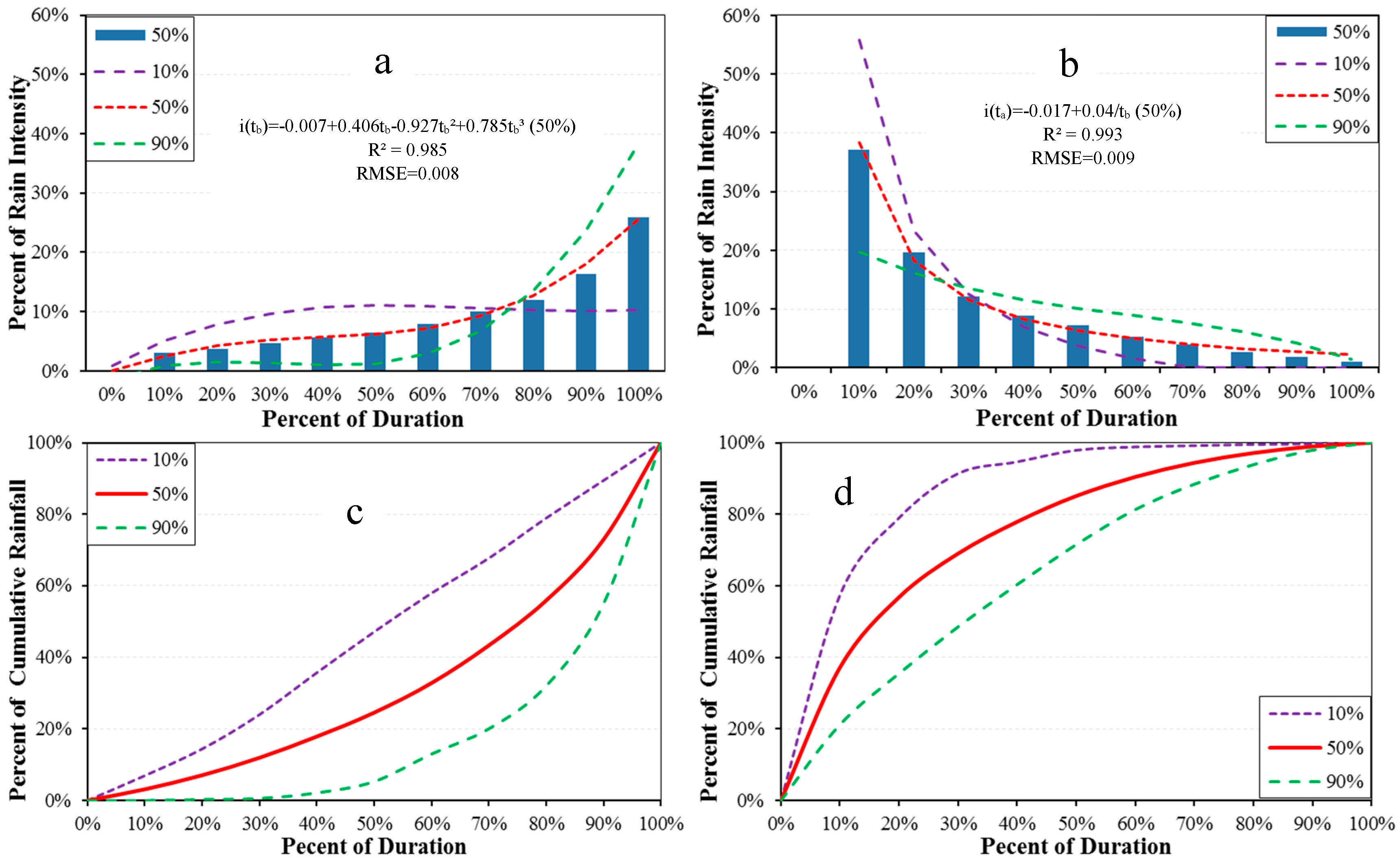
The Huff curve model is applied to describe the hyetograph of a storm event within a quartile of its normalized time of peak rainfall intensity. Instead of separating the storms into different quartiles, all storms at Site 2 from 2008 to 2012 are first separated into the rising and falling limbs. Then, a series of Huff curves are derived separately from both limbs at different probabilities, and finally form an Improved Huff curve by combining both limbs. Figure 2a,b are the developed dimensionless hyetographs using the percent of rainfall intensity at the probabilities of 10%, 50%, and 90%. Accordingly, Figure 2c,d are the curves using the percent of the cumulative rainfall depth. The mean normalized time of peak rainfall is 33 ± 5% at Site 2 (Table 3). The hyetographs of the percent of rainfall intensity at 50% are further fitted into Equations (1) and (2) by regression models for the rising and falling limbs, respectively. The fitting coefficients (R2 and RMSE) are 0.985 and 0.008 in the rising limb, and 0.993 and 0.009 in the falling limb. Both equations can be easily applied to compute the rainfall depth distribution with time once the total rainfall depth and duration are given for a drainage facility design and other purposes.
where and are the time series of rainfall intensity in the rising and falling limbs, respectively, and tb and ta represent the normalized time prior to and post the peak rainfall intensity, respectively.
The Improved Huff curves are also derived at the probability of 50% in both rising and falling limbs using the storm data within each quartile (Figure 3a,b). The first and second quartiles play a dominant role in forming the rainfall hyetograph and have a similar shape to that from all rainfall. In contrast, the hyetographs in the third and fourth quartiles show some discrepancy, especially in the falling limb.
3.2.3. Triangular Curve
The triangular curve was developed by Yen & Chow [16] for drainage design in small areas and has been widely used in watershed and urban drainage designs [16,19]. The establishment of a triangular curve is used to determine the three vertexes of the triangular hyetograph, denoted by (0, 0), (a, h), and (td, 0). The height (h) of the triangle is calculated by Equation (3) according to the area computation of a triangle.
where D is the storm total rainfall depth and td is the storm duration. Both are given values in storm or drainage facility designs.
Then, a critical step is to determine a, the time of the peak rainfall intensity, which is estimated by preserving the first moment of the rainfall depth in Equations (4) and (5) [19].
where is the first moment of the rainfall depth or the geometric center of the triangle, dj is the rainfall depth corresponding to the jth time interval, n is the number of time intervals for a storm, and is the time interval.
3.2.4. Chicago Curve
The Chicago curve is developed by intensity-duration-frequency curves for the design of sewers and drainage management [17,18,19,20,21,22]. The applied formats and constants in Guangzhou are presented in Equation (6) [14].
where I is the mean rainfall intensity, A1 is the rainfall depth with a one-year return period, C is the parameter of rainfall depth variations, P is a return period, t is the rainfall duration, and b and n are constants. The values of C, b, and n are 0.438, 11.259, and 0.750, respectively, which are adopted by the Department of Water Authority in the Guangzhou metropolitan area based on historic rainfall data from 1990 to 2010 [14]. The general equations of the rising and falling limbs are:
where and are the time series of rainfall intensity in the rising and falling limbs, respectively; tb and ta are the time before and after the peak rainfall intensity, respectively; and r is the ratio of the peak rainfall intensity time to the total duration.
3.3. Validations and Applications
The derived hyetographs are first validated by using the real hyetographs from Sites 1, 3–6. Two indices, the Root Mean Squared Error (RMSE) (Equation (8)) and Nash-Sutcliffe Efficiency (NSE) (Equation (9)), are used to evaluate their agreement [45].
where Pi is the model-predicted value, Oi is the observed value, is the mean of the observed value, and N is the number of observations.
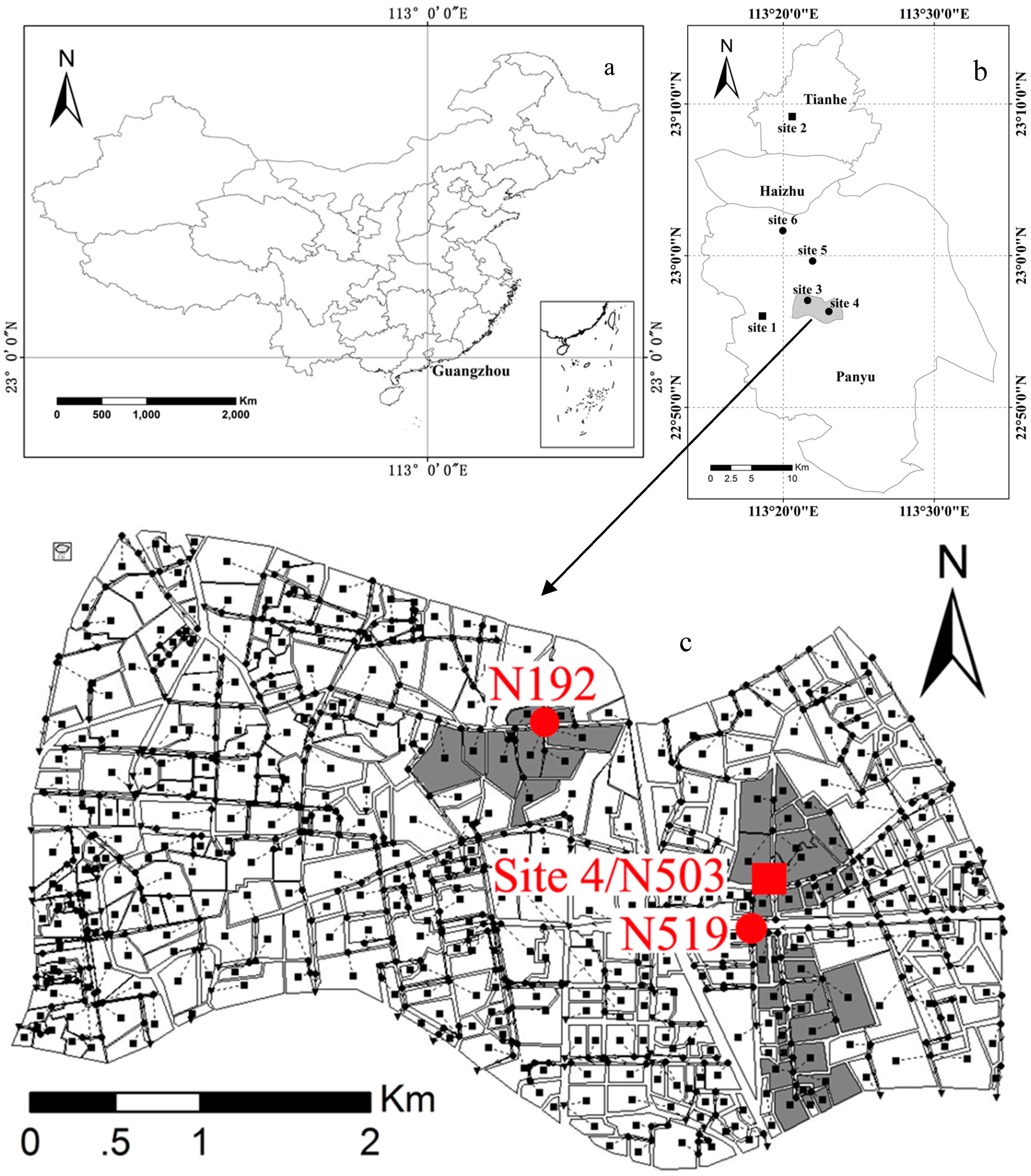
The developed design storms are further applied as inputs to the SWMM model to simulate the flooding volume in three small urban catchments. SWMM is developed by the American Environmental Protection Agency [46]. It has been widely applied in urban drainage management, flood-control facility design, water quality modeling, and so on [47,48,49,50,51,52]. In order to verify the Improved Huff curve at the rainfall depth-runoff calculation, SWMM is established in the Shiqiao Street, in the downtown area of Panyu District in the south of Guangzhou (Figure 1c). The total study area of SWMM modeling is 15.53 km2, and three catchments are selected to test the design storms, represented by Node 192, Node 503, and Node 519 (Figure 1c). The drainage boundaries of each sub-catchment are derived from detailed pipe network and fine airborne LiDAR DEM data (0.5 m grid), plus repeated field visits and validation. The selected three catchments have similar total catchment areas, but different areas in terms of their direct drainage catchment and upstream catchment (Table 4).
The SWMM model is firstly validated using the in situ measured storm rainfall and flooding volume at Site 4/Node 503. Next, the verified SWMM model is applied to simulate the flooding volume using design storms according to the storm-total rainfall depth recorded at Site 4. Finally, the simulated peak flooding volume and time at Nodes 503, 519, and 192 by all design storms and by the same storms recorded at Site 1 are compared.
4. Results
4.1. Characteristics of Historic Storms
Storm events frequently occur in the study area of a tropical climate setting. According to the given criteria, there were 71 (14/year) and 104 (21/year) storm events during the five years from 2008 to 2012 (Table 1). Site 2, which is located within the Downtown area of Tianhe District, had 46% more storm events than Site 1, especially concerning those of less than 2 h. Those storm events at Site 2 mainly (54%) concentrate in the 2nd quartile, while 44% of storm events are in the 1st quartile at Site 1 (Table 2). This large difference in short-duration storm events between the two sites is likely caused by the surrounding conditions of the urban center for Site 2 and the sub-urban area of Site 1. Similar phenomena are also found in the urban areas of Beijing [7]. However, after normalizing the rainfall duration and depth, both sites have a similar distribution with rainfall depth, time of peak intensity, and mean intensity in the rising and falling limbs, respectively (Table 3). The time of peak rainfall intensity is around 33 ± 5% of the storm duration. The rising limb displays 43 ± 5% of the total rainfall depth, with a stronger rainfall intensity than the falling limb. This suggests that the storm hyetograph is similar at both sites, which are located 25 km apart, and the design storm curve developed at one site is able to represent the overall rainfall temporal distribution at least within the study area and even in the entire Guangzhou metropolitan area.
4.2. Validations of Design Storms
The developed design storms are first validated by the storm events recorded at our own research Sites 3–6 in 2014 and 2015 (Figure 4, Table 5). Three storm events at each site are selected for a detailed comparison according to the different rainfall depths and durations of storm events. Overall, the Improved Huff curves have the best agreements with the observations, exhibiting smaller RMSE and higher NSE values than the other three curves (Table 5). The NSE of the Improved Huff curves varies from 0.94 to 0.99, except for one event (0.82) on 21 July 2015, when all design storms have a relatively lower NSE than the other events. In contrast, the Huff curves have the largest variations in terms of NSE, ranging from 0.65 to 0.99. Both Triangular and Chicago curves display a similar performance, with much larger RMSE and lower NSE values than the Improved Huff curves.
The cumulative hyetographs of one storm selected from Table 5 for each site is illustrated in Figure 4. Again, the Improved Huff curves successfully recover all of the rainfall processes recorded at the four sites. The Huff curves overestimate the observed rainfall depth at Sites 3–5, but greatly underestimate it at Site 6 prior to the peak rainfall intensity. Both the Triangular and Chicago curves tend to underestimate the rainfall prior to the peak rainfall intensity at Sites 4–6. A study in Reykjavik, the capital city of Iceland, has found that the Chicago curve underestimates the peak rainfall intensity [22]. Another study in Taiwan has shown that the Triangular curve does not satisfactorily simulate heavy storms because of its flat slope in the rising and falling limbs [53].
Besides the above events, all design storms are also validated using the 71 storm events at Site 1 from 2008 to 2012 (Table 6). The Improved Huff curves have the lowest RMSE and highest NSE values of 6.43 mm and 0.66, while they are 6.62, 7.38, and 7.57 mm and 0.63, 0.55, and 0.54 for the Huff, Triangular, and Chicago curves, respectively. Here, all design storms are derived using the parameters computed from 104 storms at Site 2. In contrast, the design storms illustrated in Figure 4 and Table 5 are derived using the parameters of each individual storm event. Therefore, the NSE values of design storms for a single storm event in Figure 4 and Table 5 are higher than those in Table 6. No matter which validation method is applied, the Improved Huff curve performs better than the others.
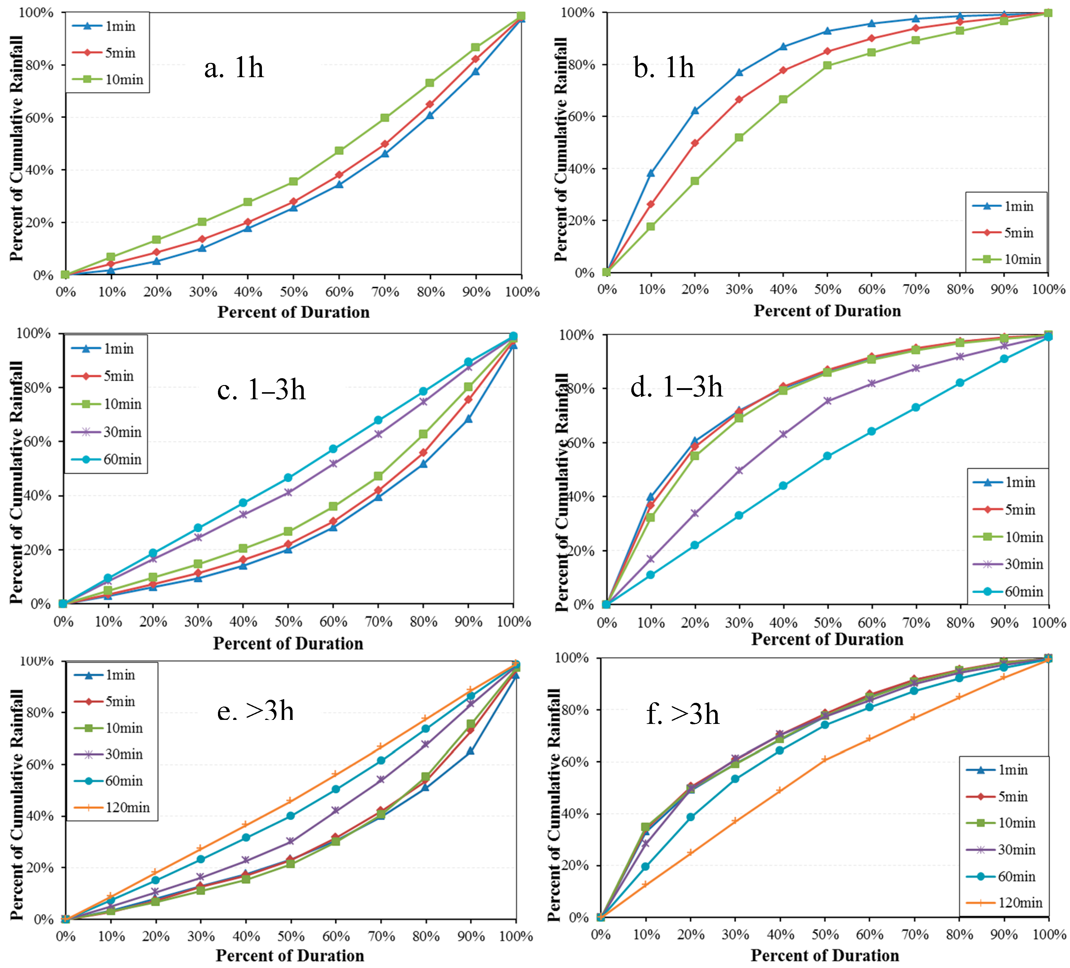
The above Huff curves are developed using the storm data at the original one-minute interval. In order to investigate the sensitivity of the Improved Huff curve to time intervals, we developed the curves by aggregating the one-minute interval data into time intervals of 5, 10, 30, 60, and 120 minutes and then compared the curves with the real storm data at Site 2. The storm events were divided into three groups by duration: <1 h, 1–3 h, and >3 h (Figure 5, Table 7). The results suggest that an optimal time interval for the original data is determined by the storm duration divided by 20, which is constrained by the 10% increment of time unit for computing the isopleths in the rising and falling limbs. For instances, for storms within 1 to 3 h, the percent of cumulative rainfall depth varies linearly with time for hourly and half-hourly data (Figure 5c,d). The mean storm duration for group 2 (1–3 h) is 100 min, and the optimal recording or computing time interval is 100/20 = 5 min. Similarly, the optimal time intervals for groups 1 (mean duration = 40 min) and 3 (mean duration = 300 min) are 2 and 15 min, respectively. The rising limb requires a smaller interval primarily due to its shorter time duration (33 ± 5%) than the falling limb. This further suggests that it is challenging to develop a storm hyetograph using hourly data in most conditions, and the rainfall depth data recorded at short-time intervals (1 min or 5 min) are required to derive a practical storm hyetograph, especially for short-duration intense storms in metropolitan areas like Guangzhou.
4.3. Applications in SWMM
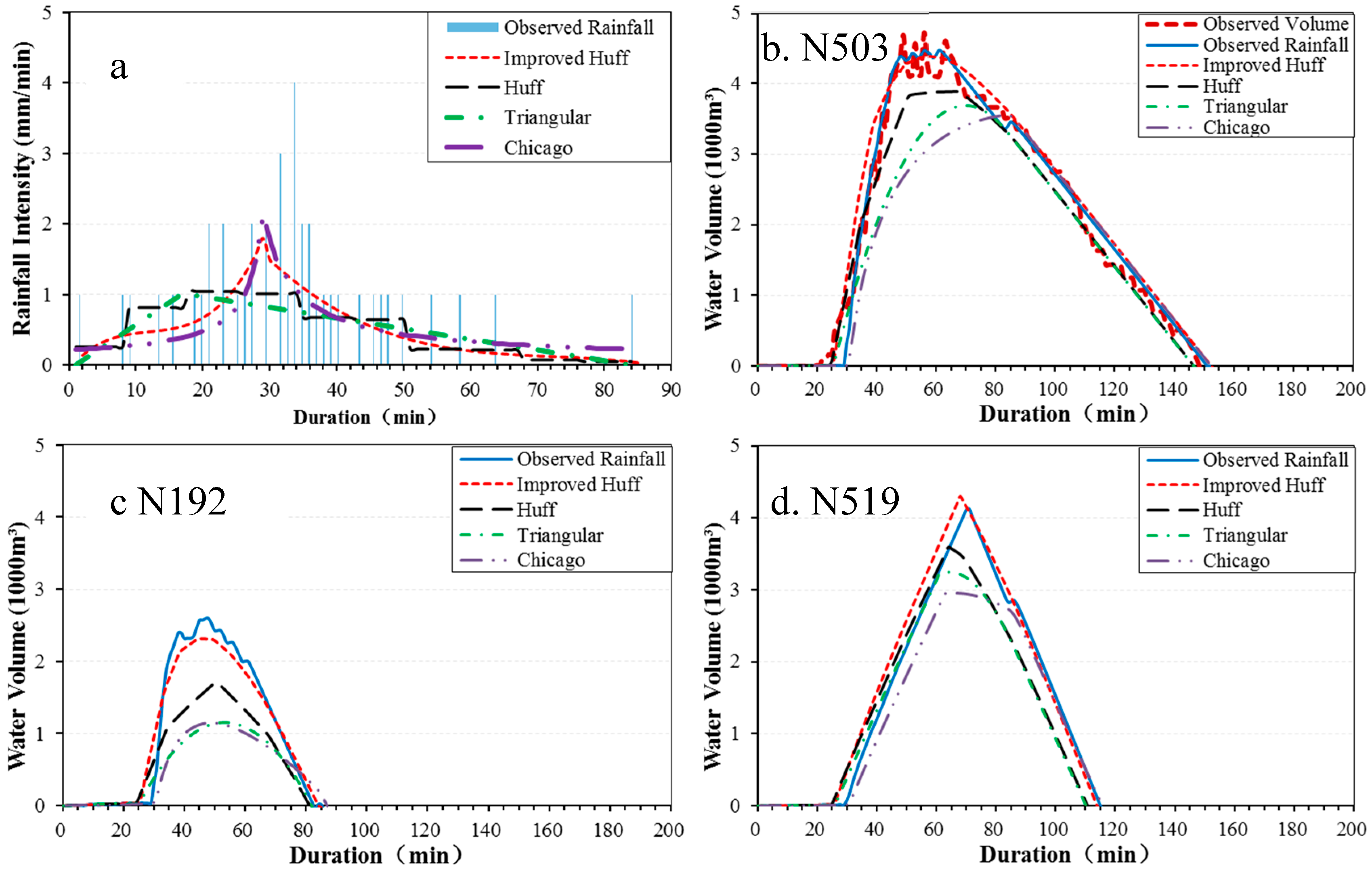
SWMM was first established and optimized using the observed rainfall and flooding volume measured at Site 4/Node503 on 2 August 2014 (Figure 6). The optimized SWMM was then utilized to simulate the flooding volume at the three nodes by using the observed rainfall and the according design storms (Figure 6b–d). At Node 503, the simulated flooding volume using the observed rainfall is in good agreement with that from the observation, especially for the four small crests (Figure 6b). The simulated peak flooding volume and time by the Improved Huff curve is also in good agreement with that from the observation. In contrast, the simulated peak flooding volumes by the Huff, Triangular, and Chicago curves all are lower than the observed values. Meanwhile, the simulated peak flooding time by the Huff, Triangular, and Chicago curves is 10, 14, and 27 min later than the real situation, respectively (Figure 6b, Table 8).
At Nodes 192 and 519, there is no observed flooding volume. The simulated flooding volumes by the four design storms are compared to those simulated by the observed rainfall depth at Site 4. The simulated flooding volumes by gauge observed rainfall and the Improved Huff curve at Node 192 are similar and smaller than those at Node 503 (Figure 6c), which is consistent with the real situations that we learned about during our field survey. This node also has the largest drainage capacity/largest pipe radius among the three nodes (Table 4). The flooding volumes reported by the Huff, Triangular, and Chicago curves are much lower than seen for the observed rainfall. The overall patterns of the simulated flooding volumes by the four design storms are similar at Node 519, and the peak flooding volume reported by the Improved Huff curve displays the best agreement with that simulated by the observed rainfall (Figure 6d, Table 8).
All of the 71 observed storm events at Site 1 from 2008 to 2012 and their design storms are applied to drive SWMM. The simulated peak flooding volume and time of the four design storms are compared to those of the observed rainfall. The results show that the improved Huff curves exhibit the best performance, followed by the original Huff curves, and then the Chicago and Triangular curves (Table 6). Again, all design storms are derived using the parameters computed from the 101 storms at Site 2.
5. Discussion
5.1. Urban Flooding
There are generically two types of urban flooding. The first type of flooding is caused by a large stream flow due to long and continuous heavy rainfall in the upstream area of the cities, such as the typhoon-brought heavy rainfall in the Guangdong province. In such cases, the drainage system in the cities plays a small role. The other type of flooding is mainly caused by short and intense rainfall, which is the primary study target in this study. The large rainfall-runoff generated within a short time cannot be drained immediately by the drainage system and thus inundates the urban streets, which is also called waterlogging in some literature [54].
Why does waterlogging frequently occur in most cities in China? Global warming is often attributed as a scapegoat. The drainage system is mandatory in urban planning and community constructions, and there are all kinds of laws and regulations on drainage design in China [13,15,55]. In our preliminary study in the same area as in this study, we simulated the runoff by SWMM with real storm rainfall and found that the drainage capacity of the pipe was below the grade that is classified in construction. Then, we examined the design storms recommended in the pipe construction code [15], such as the Triangular and Chicago curves, and found similar results as demonstrated in this study (Figure 4 and Figure 6, Table 8). These recommended curves underestimate the peak rainfall intensity, resulting in a lower peak flooding volume and thus a lower drainage capacity demand in drainage facility design for the same return period.
5.2. Improvement to the Huff Curve
It is quite challenging (if not impossible) to describe the storm hyetograph using a single design storm. A set of Huff curves are developed to describe the storm hyetographs for Peninsular Malaysia, where the majority (80%) of storms are between 3 and 6 h, belonging to the 2nd quartile [29]. Huff curves represent the temporal characteristics of rainfall quite well, although four types of Huff curves at different probabilities are required within the four quartiles [56]. Similarly, most storms (75%) are less than 3 h and dominate in the 2nd (47%) and 1st (37%) quartiles in Guangzhou (Table 1 and Table 2). Thus, the Huff curves are investigated in this study to represent the storm hyetographs using minute-interval rainfall data. However, whilst the Huff curves work well in some cases, they work badly in other cases (Figure 4 and Figure 6; Table 5 and Table 8). How could we improve the Huff curve to be better representative of the temporal distribution of all storm rainfall depth?
The time of peak rainfall has a critical influence on the analysis of hyetographs [30]. The rainfall intensity exponentially decreases on both sides of the peak rainfall in the Chicago curve [32]. The Monte Carlo method could better simulate the storm hyetograph separately in the rising and falling limbs [31]. The normalized time of peak rainfall is similar at 33 ± 5% for both sites (Table 3). The rising limb (0.64 ± 0.24 mm/min) has much stronger rainfall intensity than the falling limb (0.34 ± 0.05 mm/min). Therefore, we separate the storms into the rising and falling limbs at the time of peak rainfall and then compute the Huff curves separately for both limbs in this study.
The storm events are firstly classified into the 1st, 2nd, 3rd, and 4th quartiles according to the time of peak rainfall. Each storm event is further divided into the rising and falling limb within each quartile, within which a set of Huff curves are derived at different probabilities for both limbs. The Huff curves for all storms in both limbs are quite similar with those for storms in the 1st and 2nd quartiles (Figure 3), which include 84% of all storm events (Table 2). The Huff curves in the rising limb for the 3rd and 4th quartiles are also similar to that for all storms, and they slightly deviate from the total Huff curve in the falling limb. Too many options for the different Huff curves in the four quartiles always generate challenges and even confusion to civil engineers in practice. Therefore, considering the limited storm events in the 3rd and 4th quartiles and their slight derivation, the total Huff curves derived separately for the rising and falling limbs from all storm events are recommended in this study. The Huff curves for both limbs are finally combined together to form a full storm hyetograph, which is known as the Improved Huff curve in this study.
The Improved Huff curve could better represent the storm hyetographs recorded at rain gauges than the original Huff curve, the Triangular curve, and the Chicago curve (Figure 4, Table 5 and Table 6). This Improved Huff curve presents point-developed curves by using five-year data from one site and is verified at several neighboring sites. More sites and a longer period of time are needed to verify the curves in future studies.
The Triangular curve does not work well in our validation. One possible reason for this is that the Triangular curve is relatively flat on both sides of the peak rainfall and is often used in arid and semi-arid areas [19]. A double Triangular curve was tested to simulate the typhoon-related storms in Taiwan, China, and the central triangle of the double Triangular curve can better simulate the peak rainfall intensity than a single Triangular curve [53]. This is a possible option to improve the single Triangular curve to better represent the storm hyetographs in South China and is scheduled in our further study.
The Chicago curve is applied using constants recommended by the local water authority in this study [14]. These constants are derived from rainfall data during 1990–2010. The constants required in the Chicago curve equations may differ in different regions and climate settings and vary with the climate change, even in the same region [23]. This study does not try to apply or derive new constants by using the minute-interval rainfall depth data and this is another possible direction for our continuing study.
5.3. Application of the Improved Huff Curve
SWMM is established to verify the Improved Huff curve at the rainfall-runoff calculation (Figure 6; Table 6 and Table 8). The optimal model parameters are obtained by comparing the flooding volume between the street observations at Node 503 and SWMM simulations using the storm data at Site 4. Thus, the flooding volumes simulated by SWMM using different design storm hyetographs could represent the real situations to some extent. Of course, more storm events data could provide better model parameters and simulations [47].
The Improved Huff curve displays a better performance in SWMM than the Huff, Triangular, and Chicago curves at the three small urban catchments in the Panyu District, Guangzhou. More studies in other districts are needed to verify the results obtained in this study. After further validation, the Improved Huff curve will have great applications in drainage design in the metropolitan area of Guangzhou, other urban areas in the Guangdong province, and even in Southern China, where there are similar climate settings. Of course, the fitting coefficients or equations must be derived from the local storm data in different cities with optimal time intervals of one to five minutes.
6. Conclusions
China faces severe challenges in urban flooding due to its dramatic urbanization and relatively poor storm water management. A partial reason for this phenomenon in China is that the recommended design storms underestimate the rainfall intensity before the peak rainfall, resulting in a lower peak flooding volume and thus a lower drainage capacity demand in drainage facility design for the return period. The design storms vary with different regions and climatic conditions. This study derives a storm hyetograph to represent the temporal distributions of rainfall depth in the metropolitan area of Guangzhou by improving the Huff curve. The results are summarized below.
The Huff curve is improved by separately describing the rising and falling limbs instead of classifying the storms into four quartiles. The time of peak rainfall is at 33 ± 5% for both sites and has a critical influence on the classification of hyetographs. The rising limb has a much stronger rainfall intensity (0.64 ± 0.24 mm/min) and slightly lower rainfall depth (43 ± 5% of total rainfall depth) than the falling limb (0.34 ± 0.05 mm/min). Most (84%) of the storm events are in the 1st and 2nd quartiles, whose Huff curves are dominant and similar to those for all storms in both limbs. The Huff curves for both limbs are combined together to form a full storm hyetograph, which is known as the Improved Huff curve in this study.
The optimal time intervals are one to five minutes to derive a practical storm hyetograph, especially for short-duration and intense storms in metropolitan areas like Guangzhou. It is challenging to develop urban storm hyetographs using hourly data in most conditions. All design storms except for the Chicago Curve are derived using the minute-interval rainfall data in this study.
The Improved Huff curve works best in simulations of hyetographs and hydrographs, followed by the Huff curves, and then the Chicago curves and Triangular curves. The peak flooding volumes simulated using the Huff, Triangular, and Chicago curves as inputs to SWMM are lower than that presented by the observed rainfall, i.e., underestimating the rainfall intensity and resulting in a lower peak flooding volume.
The Improved Huff curve has great potential in storm water management such as flooding risk mapping and drainage facility design after further validation. The Improved Huff curve presents point-developed curves by using five-year data from one site and is verified at several neighboring sites in this study. More site data with longer periods are needed to verify the Improved Huff curves in future study.
Acknowledgments
This study was partially supported by the Water Resource Science and Technology Innovation Program of Guangdong Province (#2016-19), and the National Natural Science Foundation of China (#41371404; #41301419), and the Science and Technology Program of Guangzhou (#1561000154). We thank all researchers and staff for providing and maintaining the meteorological data, SWMM model, and the model required data from all agencies. We would like to express our appreciation to the Water Editorial Office and the three anonymous reviewers for their valuable comments and suggestions.
Author Contributions
Cuilin Pan performed the experiments, processed the data, analyzed the results, and wrote the manuscript; Xianwei Wang designed experiments, analyzed the results, and wrote and revised the manuscript; Lin Liu, Huabing Huang, and Dashan Wang contributed to obtaining the in situ measurements, set up the SWMM model, improved the experiments, and revised the manuscript.
Conflicts of Interest
The authors declare no conflict of interest.
References
- Ahmed, S.I.; Rudra, R.P.; Gharabaghi, B.; Mackenzie, K.; Dickinson, W.T. Within-storm rainfall distribution effect on soil erosion rate. ISRN Soil Sci. 2012, 2012, 1–7. [Google Scholar] [CrossRef]
- Bonta, J.V. Development and utility of Huff curves for disaggregating precipitation amounts. Appl. Eng. Agric. 2004, 20, 641–653. [Google Scholar] [CrossRef]
- Dolšak, D.; Bezak, N.; Šraj, M. Temporal characteristics of rainfall events under three climate types in Slovenia. J. Hydrol. 2016, 541, 1395–1405. [Google Scholar] [CrossRef]
- Park, D.; Jang, S.; Roesner, L.A. Evaluation of multi-use stormwater detention basins for improved urban watershed management. Hydrol. Processes 2014, 28, 1104–1113. [Google Scholar] [CrossRef]
- Kang, M.S.; Goo, J.H.; Song, I.; Chun, J.A.; Her, Y.G.; Hwang, S.W.; Park, S.W. Estimating design floods based on the critical storm duration for small watersheds. J. Hydro-Environ. Res. 2013, 7, 209–218. [Google Scholar] [CrossRef]
- Grimaldi, S.; Petroselli, A.; Serinaldi, F. Design hydrograph estimation in small and ungauged watersheds: Continuous simulation method versus event-based approach. Hydrol. Process. 2012, 26, 3124–3134. [Google Scholar] [CrossRef]
- Yang, L.; Tian, F.; Smith, J.A.; Hu, H. Urban signatures in the spatial clustering of summer heavy rainfall events over the Beijing metropolitan region. J. Geophys. Res. 2014, 119, 1203–1217. [Google Scholar] [CrossRef]
- Shastri, H.; Paul, S.; Ghosh, S.; Karmakar, S. Impacts of urbanization on Indian summer monsoon rainfall extremes. J. Geophys. Res. 2015, 120, 495–516. [Google Scholar] [CrossRef]
- Madsen, H.; Lawrence, D.; Lang, M.; Martinkova, M.; Kjeldsen, T.R. Review of trend analysis and climate change projections of extreme precipitation and floods in Europe. J. Hydrol. 2014, 519, 3634–3650. [Google Scholar] [CrossRef]
- Jato-Espino, D.; Sillanpää, N.; Charlesworth, S.; Andrés-Doménech, I. Coupling GIS with stormwater modelling for the location prioritization and hydrological simulation of permeable pavements in urban catchments. Water 2016, 8, 451. [Google Scholar] [CrossRef]
- Liu, L.; Liu, Y.; Wang, X.; Yu, D.; Liu, K.; Huang, H.; Hu, G. Developing an effective 2-D urban flood inundation model for city emergency management based on cellular automata. Nat. Hazards Earth Syst. Sci. 2015, 15, 381–391. [Google Scholar] [CrossRef]
- Yang, L.; Scheffran, J.; Qin, H.; You, Q. Climate-related flood risks and urban responses in the Pearl River Delta, China. Reg. Environ. Chang. 2015, 15, 379–391. [Google Scholar] [CrossRef]
- China Meteorological Administration (CMA). Regulations on Short-Term and Near-Real Time Forecasting Operations, No. (2010)19; China Meteorological Administration: Beijing, China, 2011. Available online: http://www.njqxj.gov.cn/xwxt/ztjd/zcqnwmh/gzzd/201308/t20130819_1089526.html (accessed on 18 April 2015).
- Guangzhou Bureau of Water Authority (GBWA). The Rainstorm Formula and Calculation Chart in Guangzhou Downtown, No. (2011)214; Guangzhou Bureau of Water Authority: Guangzhou, China, 2011. Available online: http://www.cma.gov.cn/2011xwzx/2011xxdqxywtx/2011xzhgcxt/201110/t20111029_141510.html (accessed on 10 April 2015).
- Ministry of Housing and Urban-Rural Development of the People’s Republic of China (MOHURD). Code for Design of Outdoor Wastewater Engineering, GB 50014-2006; Ministry of Housing and Urban-Rural Development of the People’s Republic of China: Beijing, China, 2006. Available online: http://www.mohurd.gov.cn/wjfb/200610/t20061031_155882.html (accessed on 22 April 2015).
- Yen, B.C.; Chow, V.T. Design hyetographs for small drainage structures. J. Hydraul. Div. ASCE 1980, 106, 1055–1076. [Google Scholar]
- Keifer, G.J.; Chu, H.H. Synthetic storm pattern for drainage design. J. Hydraul. Div. ASCE 1957, 83, 1–25. [Google Scholar]
- Soil Conservation Service (SCS). Urban hydrology for small watersheds. In Technical Release 55; U.S. Department of Agriculture, Washington, D.C. Soil Conservation Service: Washington, DC, USA, 1986. [Google Scholar]
- Ellouze, M.; Habib, A.; Riadh, S. A triangular model for the generation of synthetic hyetographs. Hydrol. Sci. J. 2009, 54, 287–299. [Google Scholar] [CrossRef]
- Asquith, W.H.; Bumgarner, J.R.; Fahlquist, L.S. A triangular model of dimensionless runoff producing rainfall hyetographs in Texas. J. Am. Water Resour. Assoc. 2003, 39, 911–921. [Google Scholar] [CrossRef]
- Palynchuk, B.A.; Guo, Y. A probabilistic description of rain storms incorporating peak intensities. J. Hydrol. 2011, 409, 71–80. [Google Scholar] [CrossRef]
- Hlodversdottir, A.O.; Bjornsson, B.; Andradottir, H.O.; Eliasson, J.; Crochet, P. Assessment of flood hazard in a combined sewer system in Reykjavik city centre. Water Sci. Technol. 2015, 71, 1471–1477. [Google Scholar] [CrossRef] [PubMed]
- Berggren, K.; Packman, J.; Ashley, R.; Viklander, M. Climate changed rainfalls for urban drainage capacity assessment. Urban Water J. 2014, 11, 543–556. [Google Scholar] [CrossRef]
- Soil Conservation Service (SCS). National Engineering Handbook, Section 4; U.S. Department of Agriculture, Washington, D.C. Soil Conservation Service: Washington, DC, USA, 1972.
- Yang, X.; Zhu, D.; Li, C.; Liu, Z. Establishment of design hyetographs based on risk probability models. J. Hydraul. Eng. 2013, 44, 542–548. (In Chinese) [Google Scholar]
- Vieux, B.E.; Vieux, J.E. Continuous Distributed Modeling of LID/GI: Scaling from Site to Watershed. In Proceedings of the International Low Impact Development Conference, Huston, TX, USA, 17–21 January 2015; pp. 285–294. [Google Scholar]
- HEC-Hydrologic Modeling System (HEC-HMS). User’s Manual. Version 4.0; US Army Corps of Engineers Hydrologic Engineering Center: Davis, CA, USA, 2013.
- Yin, S.Q.; Xie, Y.; Nearing, M.A.; Guo, W.L.; Zhu, Z.Y. Intra-Storm Temporal Patterns of Rainfall in China Using Huff Curves. Trans. ASABE 2016, 59, 1619–1632. [Google Scholar]
- Azli, M.; Rao, A.R. Development of Huff curves for Peninsular Malaysia. J. Hydrol. 2010, 388, 77–84. [Google Scholar] [CrossRef]
- Lin, G.; Chen, L.; Kao, S. Development of regional design hyetographs. Hydrol. Process. 2005, 19, 937–946. [Google Scholar] [CrossRef]
- Kottegoda, N.T.; Natale, L.; Raiteri, E. Monte Carlo Simulation of rainfall hyetographs for analysis and design. J. Hydrol. 2014, 519, 1–11. [Google Scholar] [CrossRef]
- Niemczynowicz, J. Impact of the greenhouse effect on sewerage systems—Lund case study. Hydrol. Sci. J. 1989, 34, 651–666. [Google Scholar] [CrossRef]
- Liu, T.; Zhang, Y.H.; Xu, Y.J.; Lin, H.L.; Xu, X.J.; Luo, Y.; Xiao, J.; Zeng, W.L.; Zhang, W.F.; Chu, C.; et al. The effects of dust–haze on mortality are modified by seasons and individual characteristics in Guangzhou, China. Environ. Pollut. 2014, 187, 116–123. [Google Scholar] [CrossRef] [PubMed]
- Xie, L.; Wei, G.; Deng, W.; Zhao, X. Daily δ18O and δD of precipitations from 2007 to 2009 in Guangzhou, South China: Implications for changes of moisture sources. J. Hydrol. 2011, 400, 477–489. [Google Scholar] [CrossRef]
- Fan, F.; Fan, W. Understanding spatial-temporal urban expansion pattern (1990–2009) using impervious surface data and landscape indexes: A case study in Guangzhou (China). J. Appl. Remote Sens. 2014, 8, 083609. [Google Scholar] [CrossRef]
- Wu, H.; Huang, G.; Meng, Q.; Zhang, M.; Li, L. Deep Tunnel for regulating combined sewer overflow pollution and flood disaster: A case study in Guangzhou City, China. Water 2016, 8, 329. [Google Scholar] [CrossRef]
- Lu, W. Problems and suggestions on Guangzhou urban flood disaster management. Chin. Public Adm. 2014, 343, 106–108. (In Chinese) [Google Scholar]
- Bonta, J.V.; Rao, A.R. Factors affecting development of Huff curves. Trans. ASAE 1987, 30, 1689–1693. [Google Scholar] [CrossRef]
- Todisco, F. The internal structure of erosive and non-erosive storm events for interpretation of erosive processes and rainfall simulation. J. Hydrol. 2014, 519, 3651–3663. [Google Scholar] [CrossRef]
- Bonta, J.V.; Rao, A.R. Fitting equations to families of dimensionless cumulative hyetographs. Trans. ASAE 1988, 31, 756–760. [Google Scholar] [CrossRef]
- Bonta, J.V.; Rao, A.R. Regionalization of storm hyetographs. Trans. ASAE 1989, 25, 211–217. [Google Scholar] [CrossRef]
- Terranova, O.G.; Iaquinta, P. Temporal properties of rainfall events in Calabria (southern Italy). Nat. Hazards Earth Syst. Sci. 2011, 11, 751–757. [Google Scholar] [CrossRef]
- Terranova, O.G.; Gariano, S.L. Rainstorms able to induce flash floods in a Mediterranean-climate region (Calabria, southern Italy). Nat. Hazards Earth Syst. Sci. 2014, 14, 2423–2434. [Google Scholar] [CrossRef]
- Huff, F.A. Time distributions of heavy rainstorms in Illinois. In Illinois State Water Survey, Circular 173; Illinois State Water Survey: Champaign, IL, USA, 1990. [Google Scholar]
- Thapa, R.B.; Watanabe, M.; Motohka, T.; Shimada, M. Potential of high-resolution ALOS–PALSAR mosaic texture for aboveground forest carbon tracking in tropical region. Remote Sens. Environ. 2015, 160, 122–133. [Google Scholar] [CrossRef]
- United States Environmental Protection Agency (EPA). Storm Water Management Model Applications Manual; United States Environmental Protection Agency: Washington, DC, USA, 2009.
- Versini, P.A.; Ramier, D.; Berthier, E.; de Gouvello, B. Assessment of the hydrological impacts of green roof: From building scale to basin scale. J. Hydrol. 2015, 524, 562–575. [Google Scholar] [CrossRef]
- Croci, S.; Paoletti, A.; Tabellini, P. URBFEP Model for Basin Scale Simulation of Urban Floods Constrained by Sewerage’s Size Limitations. Procedia Eng. 2014, 70, 389–398. [Google Scholar] [CrossRef]
- Li, F.; Duan, H.; Yan, H.; Tao, T. Multi-Objective Optimal Design of Detention Tanks in the Urban Stormwater Drainage System: Framework Development and Case Study. Water Resour. Manag. 2015, 29, 2125–2137. [Google Scholar] [CrossRef]
- Palla, A.; Gnecco, I. Hydrologic modeling of Low Impact Development systems at the urban catchment scale. J. Hydrol. 2015, 528, 361–368. [Google Scholar] [CrossRef]
- Martínez-Solano, F.; Iglesias-Rey, P.; Saldarriaga, J.; Vallejo, D. Creation of an SWMM toolkit for its application in urban drainage networks optimization. Water 2016, 8, 259. [Google Scholar] [CrossRef]
- Ngo, T.; Yoo, D.; Lee, Y.; Kim, J. Optimization of upstream detention reservoir facilities for downstream flood mitigation in urban areas. Water 2016, 8, 290. [Google Scholar] [CrossRef]
- Lee, K.T.; Ho, J.Y. Design hyetograph for typhoon rainstorms in Taiwan. J. Hydrol. Eng. 2008, 7, 647–651. [Google Scholar] [CrossRef]
- Xie, Z.; Du, Q.; Ren, F.; Zhang, X.; Jamiesone, S. Improving the forecast precision of river stage spatial and temporal distribution using drain pipeline knowledge coupled with BP artificial neural networks: A case study of Panlong River, Kunming, China. Nat. Hazards 2015, 77, 1081–1102. [Google Scholar] [CrossRef]
- Ministry of Housing and Urban-Rural Development of the People’s Republic of China (MOHURD). Code of Urban Wastewater Engineering Planning, GB 50318–2000; Ministry of Housing and Urban-Rural Development of the People’s Republic of China: Beijing, China, 2000. Available online: http://www.czs.gov.cn/ghj/zcfg/jsbzygf/content_195311.html (accessed on 15 April 2015).
- Bonnin, G.M.; Martin, D.; Lin, B.; Paryzbok, T.; Yekta, M.; Riley, D. Precipitation Frequency Atlas of the United States; Version 3.0; NOAA Atlas 14; National Weather Service: Silver Springs, MD, USA, 2006; Volume 2.
Figure 1.
The locations of Guangzhou (a); meteorological sites (b); and the three selected nodes and their catchment area/ modeling areas by SWMM in Panyu District (c). Street flooding water depth is recorded near Site 4/Node 503 by a wireless electronic water depth meter.
Figure 1.
The locations of Guangzhou (a); meteorological sites (b); and the three selected nodes and their catchment area/ modeling areas by SWMM in Panyu District (c). Street flooding water depth is recorded near Site 4/Node 503 by a wireless electronic water depth meter.

Figure 2.
Comparisons of rainfall intensity and cumulative rainfall percent derived by the Improved Huff curve at three probabilities (10%, 50%, and 90%) for the rising limb (a,c), and the falling limb (b,d), which are separated by the time of peak rainfall (33%) at Site 2.
Figure 2.
Comparisons of rainfall intensity and cumulative rainfall percent derived by the Improved Huff curve at three probabilities (10%, 50%, and 90%) for the rising limb (a,c), and the falling limb (b,d), which are separated by the time of peak rainfall (33%) at Site 2.

Figure 3.
The Huff curves for the rising (a) and falling (b) limbs at a probability of 50% by all storm events and by those within the four quartiles at Site 2.
Figure 3.
The Huff curves for the rising (a) and falling (b) limbs at a probability of 50% by all storm events and by those within the four quartiles at Site 2.
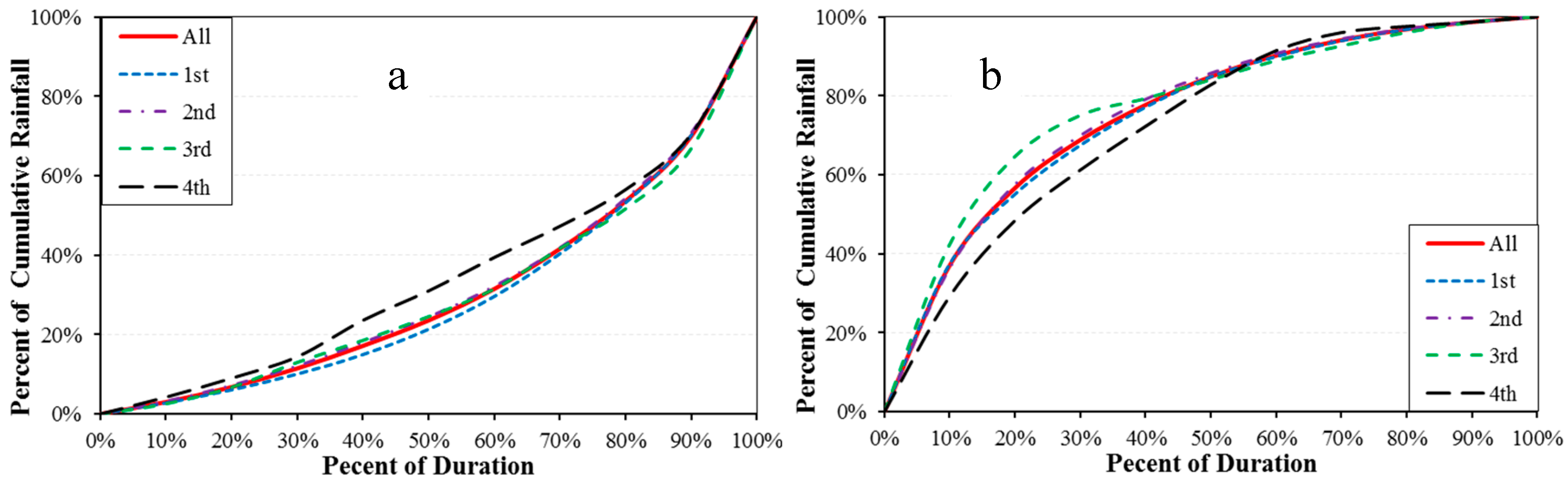
Figure 4.
Comparisons of cumulative rainfall between ground observations and the design storms for the storm events at Site 3 on 21 September 2015 (a); at Site 4 on 25 May 2015 (b); at Site 5 on 3 October 2015 (c); and at Site 6 on 21 July 2015 (d).
Figure 4.
Comparisons of cumulative rainfall between ground observations and the design storms for the storm events at Site 3 on 21 September 2015 (a); at Site 4 on 25 May 2015 (b); at Site 5 on 3 October 2015 (c); and at Site 6 on 21 July 2015 (d).
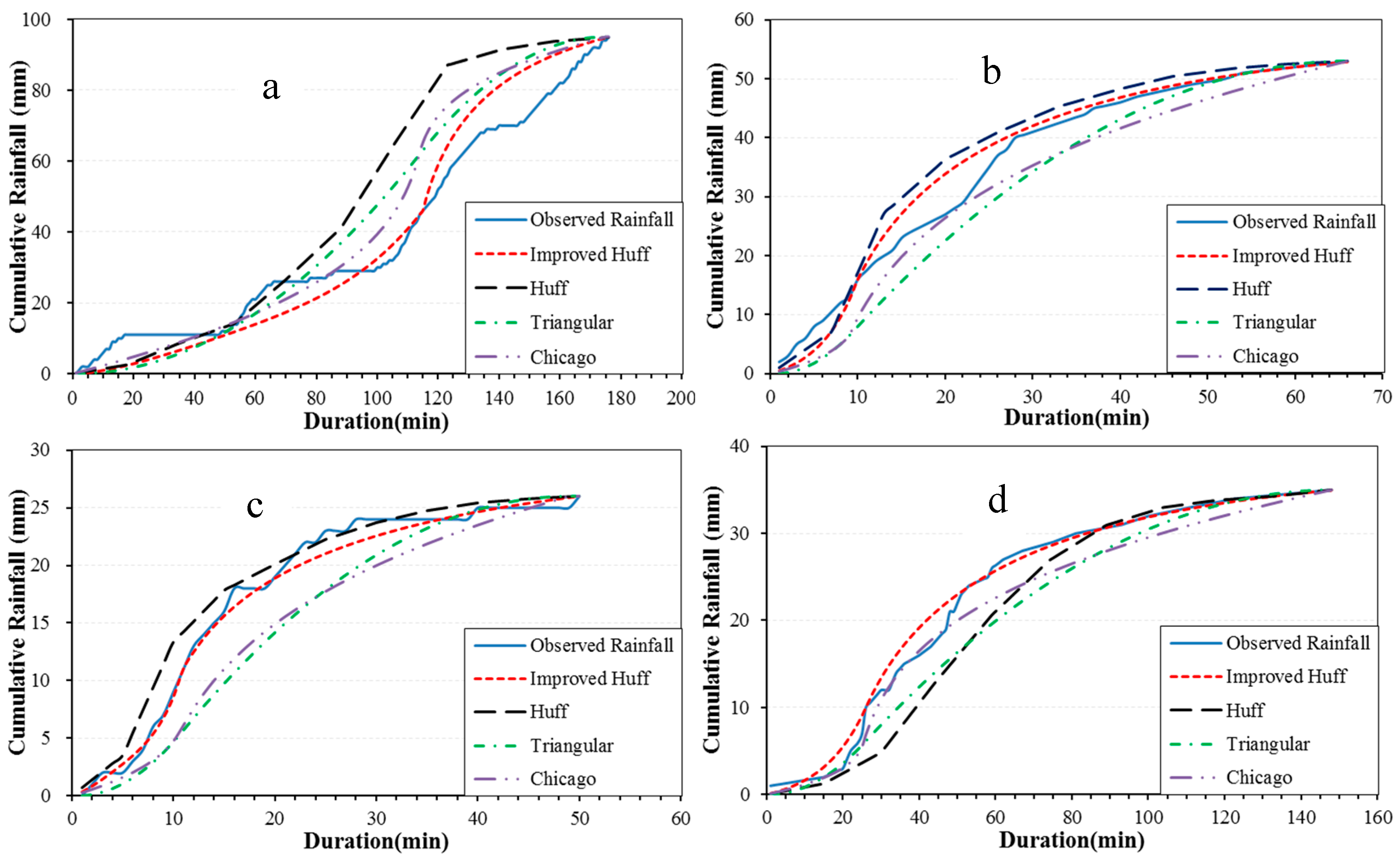
Figure 5.
Percent of cumulative rainfall depth derived by the Improved Huff curves (probability 50%) using different time intervals for three groups (rainfall duration: 1 h, 1–3 h, and >3 h) of storms from 2008 to 2012 at Site 2. Plots (a,c,e) are for the rising limb, and plots (b,d,f) are for the falling limb.

Figure 6.
Comparisons of hyetographs (a) and the according ground measured and simulated flooding volume by SWMM using different hyetographs at Node 503 (b), Node 192 (c) and Node 519 (d) for the storm event recorded at Site 4 on 2 August 2014, with total rainfall of 42 mm and duration of 84 min.
Figure 6.
Comparisons of hyetographs (a) and the according ground measured and simulated flooding volume by SWMM using different hyetographs at Node 503 (b), Node 192 (c) and Node 519 (d) for the storm event recorded at Site 4 on 2 August 2014, with total rainfall of 42 mm and duration of 84 min.

Table 1.
The number of storms in different durations at two sites for the period 2008–2012.
| Rain Gauges | Duration (h) | |||||||
|---|---|---|---|---|---|---|---|---|
| <1 | 1–2 | 2–3 | 3–4 | 4–5 | 5–6 | >6 | Total | |
| Site 1 (Sub-urban) | 12 | 27 | 15 | 3 | 6 | 5 | 3 | 71 |
| Site 2 (Urban) | 25 | 37 | 16 | 11 | 6 | 5 | 4 | 104 |
| Total | 37(21%) | 64(36%) | 31(18%) | 14(8%) | 12(7%) | 10(6%) | 7(4%) | 175 |
Table 2.
The number of storms in each quartile defined according to the occurrence of peak rainfall considering a normalized time at two sites for the period 2008–2012.
Table 2.
The number of storms in each quartile defined according to the occurrence of peak rainfall considering a normalized time at two sites for the period 2008–2012.
| Quartiles | 1st | 2nd | 3rd | 4th | Total |
|---|---|---|---|---|---|
| Site 1 | 31(44%) | 27(38%) | 9(13%) | 4(6%) | 71 |
| Site 2 | 33(32%) | 56(54%) | 8(8%) | 7(7%) | 104 |
| Total | 64(37%) | 83(47%) | 17(10%) | 11(6%) | 175 |
Table 3.
Statistics of the rising and falling limbs for storm events at Sites 1 and 2 from 2008 to 2012.
Table 3.
Statistics of the rising and falling limbs for storm events at Sites 1 and 2 from 2008 to 2012.
| Title | Rainfall Depth (%) | Rainfall Duration (%) | Intensity (mm/min) | |||
|---|---|---|---|---|---|---|
| Rising | Falling | Rising | Falling | Rising | Falling | |
| Site 1 | 45 ± 5% | 55 ± 5% | 33 ± 5% | 67 ± 5% | 0.66 ± 0.26 | 0.36 ± 0.03 |
| Site 2 | 41 ± 4% | 59 ± 4% | 33 ± 5% | 67 ± 5% | 0.62 ± 0.23 | 0.32 ± 0.07 |
| Mean | 43 ± 5% | 57 ± 5% | 33 ± 5% | 67 ± 5% | 0.64 ± 0.24 | 0.34 ± 0.05 |
Table 4.
Direct Catchment Area (DCA), Upstream Catchment Area (UCA), Total Catchment Area (TCA), and Drainage Capacity (DC) of the three selected nodes.
Table 4.
Direct Catchment Area (DCA), Upstream Catchment Area (UCA), Total Catchment Area (TCA), and Drainage Capacity (DC) of the three selected nodes.
| Node | DCA (ha) | UCA (ha) | TCA (ha) | DC (m3/s) |
|---|---|---|---|---|
| 503 | 8.8 | 26.2 | 35.0 | 0.88 |
| 192 | 10.1 | 27.3 | 37.4 | 1.76 |
| 519 | 2.4 | 40.5 | 43.0 | 1.69 |
Table 5.
RMSE and NSE values computed between design storms and observed rainfall at Sites 3-6, where the observed storm data are not used to develop design storms. Both the Improved Huff and original Huff curves represent those at a probability of 50%.
Table 5.
RMSE and NSE values computed between design storms and observed rainfall at Sites 3-6, where the observed storm data are not used to develop design storms. Both the Improved Huff and original Huff curves represent those at a probability of 50%.
| Site | Date | Rainfall Depth (mm) | Duration (min) | Intensity (mm/h) | Index | Improved Huff | Huff | Triangular | Chicago |
|---|---|---|---|---|---|---|---|---|---|
| 3 | 19 August 2014 | 40 | 28 | 86 | RMSE | 1.08 | 1.22 | 4.91 | 4.33 |
| NSE | 0.99 | 0.99 | 0.87 | 0.88 | |||||
| 21 September 2015 | 95 | 175 | 33 | RMSE | 6.92 | 16.43 | 10.79 | 9.75 | |
| NSE | 0.94 | 0.65 | 0.85 | 0.88 | |||||
| 03 October 2015 | 55 | 136 | 24 | RMSE | 3.70 | 9.34 | 3.56 | 4.09 | |
| NSE | 0.96 | 0.75 | 0.96 | 0.95 | |||||
| 4 | 02 August 2014 | 42 | 84 | 30 | RMSE | 2.75 | 3.53 | 5.39 | 4.90 |
| NSE | 0.97 | 0.94 | 0.88 | 0.90 | |||||
| 11 May 2015 | 78 | 97 | 48 | RMSE | 5.58 | 8.54 | 14.25 | 12.25 | |
| NSE | 0.95 | 0.87 | 0.65 | 0.74 | |||||
| 25 May 2015 | 53 | 66 | 48 | RMSE | 2.74 | 3.91 | 4.60 | 3.87 | |
| NSE | 0.97 | 0.94 | 0.91 | 0.93 | |||||
| 5 | 16 May 2015 | 27 | 65 | 25 | RMSE | 1.74 | 2.80 | 2.05 | 1.22 |
| NSE | 0.94 | 0.83 | 0.91 | 0.97 | |||||
| 21 July 2015 | 22 | 59 | 22 | RMSE | 2.56 | 2.89 | 2.99 | 2.64 | |
| NSE | 0.82 | 0.76 | 0.75 | 0.80 | |||||
| 03 October 2015 | 26 | 49 | 32 | RMSE | 0.85 | 1.53 | 3.56 | 3.36 | |
| NSE | 0.99 | 0.96 | 0.81 | 0.83 | |||||
| 6 | 21 June 2014 | 30 | 105 | 17 | RMSE | 1.32 | 1.62 | 3.87 | 3.63 |
| NSE | 0.95 | 0.94 | 0.55 | 0.61 | |||||
| 20 August 2014 | 34 | 125 | 16 | RMSE | 1.28 | 3.38 | 2.88 | 1.81 | |
| NSE | 0.99 | 0.92 | 0.94 | 0.98 | |||||
| 21 July 2015 | 35 | 148 | 15 | RMSE | 1.17 | 2.95 | 2.84 | 1.78 | |
| NSE | 0.99 | 0.93 | 0.94 | 0.97 |
Table 6.
Mean RMSE and NSE values between the 71 observed hyetographs at Site 1 and their design storms, and the mean relative difference of the simulated peak flooding volume (PV) and time (PT) at the three nodes by the design storms against those simulated by the 71 observed storms at Site 1. All design storms are computed using the parameters derived from the 104 storms at Site 2, together with the total rainfall depth and duration for each storm at Site 1.
| Index | Improved Huff | Huff | Triangular | Chicago | |
|---|---|---|---|---|---|
| RMSE | 6.43 | 6.62 | 7.38 | 7.57 | |
| NSE | 0.66 | 0.63 | 0.55 | 0.54 | |
| N503 | PV(%) | 2 | −12 | −22 | −17 |
| PT(%) | 19 | 24 | 45 | 41 | |
| N192 | PV(%) | −6 | −43 | −62 | −19 |
| PT(%) | 17 | 19 | 15 | 24 | |
| N519 | PV(%) | 8 | −16 | −38 | −21 |
| PT(%) | 8 | 8 | 9 | 10 | |
Table 7.
NSE, RMSE, (mm) and Relative Difference (RD) values between design storms derived by the Improved Huff curves (probability 50%) using different time intervals and observed rainfall depth for all storms at Site 2 from 2008 to 2012.
Table 7.
NSE, RMSE, (mm) and Relative Difference (RD) values between design storms derived by the Improved Huff curves (probability 50%) using different time intervals and observed rainfall depth for all storms at Site 2 from 2008 to 2012.
| Duration (h) | Title | Time Interval (min) | |||||
|---|---|---|---|---|---|---|---|
| 1 | 5 | 10 | 30 | 60 | 120 | ||
| 1 | NSE | 0.97 | 0.94 | 0.81 | |||
| RMSE | 1.32 | 2.12 | 3.80 | ||||
| RD (%) | 2 | −5 | 13 | ||||
| 1–3 | NSE | 0.94 | 0.94 | 0.94 | 0.89 | 0.75 | |
| RMSE | 2.22 | 2.24 | 2.36 | 3.61 | 5.27 | ||
| RD (%) | −2 | −3 | −3 | −5 | −13 | ||
| >3 | NSE | 0.92 | 0.92 | 0.92 | 0.92 | 0.90 | 0.82 |
| RMSE | 5.81 | 5.85 | 5.87 | 5.94 | 5.99 | 8.00 | |
| RD (%) | 2 | −3 | −3 | −4 | −4 | −10 | |
Table 8.
Peak flooding volume, time, and NSE simulated by SWMM using rainfall depths from gauge observations at Sites 4 and the considered design storms. The last four columns are the difference in the simulated peak flooding volume and time using design storms (DS) against those by gauge (G) rainfall depth. The water volume at Node 503 is computed according to the DEM and water depth recorded at Site 4/Node 503, while that at Node 192 and 519 is simulated by SWMM using gauge rainfall depth data at Site 4.
| Date Total P & T | Node | Flooding Volume & Time by Gauge Rain | Difference of Flooding Volume and Time (DS-G) | |||
|---|---|---|---|---|---|---|
| Improved Huff | Huff | Triangular | Chicago | |||
| 4733 m3 | −342 | −844 | −1044 | −1173 | ||
| 503 | 57 min | 0 | 10 | 14 | 27 | |
| NSE | 0.97 | 0.93 | 0.90 | 0.86 | ||
| 2 August 2014 | 2596 | −281 | −703 | −1313 | −1319 | |
| 42 mm | 192 | 46 | −1 | 3 | 7 | 2 |
| 84 min | NSE | 0.97 | 0.71 | 0.38 | 0.39 | |
| 4126 | 173 | −532 | −879 | −1171 | ||
| 519 | 70 | −2 | −7 | −6 | −5 | |
| NSE | 0.98 | 0.92 | 0.93 | 0.92 | ||
© 2017 by the authors. Licensee MDPI, Basel, Switzerland. This article is an open access article distributed under the terms and conditions of the Creative Commons Attribution (CC BY) license (http://creativecommons.org/licenses/by/4.0/).
Share and Cite
MDPI and ACS Style
Pan, C.; Wang, X.; Liu, L.; Huang, H.; Wang, D. Improvement to the Huff Curve for Design Storms and Urban Flooding Simulations in Guangzhou, China. Water 2017, 9, 411. https://doi.org/10.3390/w9060411
AMA Style
Pan C, Wang X, Liu L, Huang H, Wang D. Improvement to the Huff Curve for Design Storms and Urban Flooding Simulations in Guangzhou, China. Water. 2017; 9(6):411. https://doi.org/10.3390/w9060411
Chicago/Turabian StylePan, Cuilin, Xianwei Wang, Lin Liu, Huabing Huang, and Dashan Wang. 2017. "Improvement to the Huff Curve for Design Storms and Urban Flooding Simulations in Guangzhou, China" Water 9, no. 6: 411. https://doi.org/10.3390/w9060411
Note that from the first issue of 2016, this journal uses article numbers instead of page numbers. See further details here.