Optimal Combinations of Non-Sequential Regressors for ARX-Based Typhoon Inundation Forecast Models Considering Multiple Objectives


1
Department of Civil Engineering, National Ilan University, Yilan 26047, Taiwan
2
Department of Civil Engineering, National Taiwan University, Taipei 10617, Taiwan
*
Author to whom correspondence should be addressed.
Water 2017, 9(7), 519; https://doi.org/10.3390/w9070519
Submission received: 19 April 2017
/
Revised: 3 July 2017
/
Accepted: 11 July 2017
/
Published: 14 July 2017
(This article belongs to the Special Issue Applications of Remote Sensing/GIS in Water Resources and Flooding Risk Managements)
Abstract
:Inundation forecast models with non-sequential regressors are advantageous in efficiency due to their rather fewer input variables required to be processed. This type of model is nevertheless rare mainly because of the difficulty in finding the proper combination of regressors for the model to perform accurate prediction. A novel methodology is proposed in this study to tackle the problem. The approach involves integrating a Multi-Objective Genetic Algorithm (MOGA) with forecast models based on ARX (Auto-Regressive model with eXogenous inputs) to transfer the search for the optimal combination of non-sequential regressors into an optimization problem. An innovative approach to codifying any combinations of model regressors into binary strings is developed and employed in MOGA. The Pareto optimal sets of three types of models including linear ARX (LARX), nonlinear ARX with Wavelet function (NLARX-W), and nonlinear ARX with Sigmoid function (NLARX-S) are searched for by the proposed methodology. The results show that the optimal models acquired through this approach have good inundation forecasting capabilities in every aspect in terms of accuracy, time shift error, and error distribution.
1. Introduction
Typhoon is a common weather phenomenon in subtropical areas and usually occurs between July and October of each year. Heavy rainfall brought by the typhoon during the event usually results in serious inundation problems in low-lying areas, which not only causes property loss to the local population but also threatens their safety. Due to restrictions on engineering funding, structural protective measures are constrained by the designed limits. Once the typhoon scale exceeds the designed protective limit, people must rely on nonstructural means for disaster relief during the event, such as evacuating people from areas in potentially high flooding risk. Among nonstructural measures the accurate forecast of the inundation level in the areas within the next several hours is a critical factor in the decision-making and planning of disaster relief actions.
Relevant studies on inundation forecast technology are quite ample and can generally be divided into either the numerical simulation or the black-box modeling. The numerical simulation is based on theoretical deduction through the understanding of the mechanism from rainfall to inundation. The advantage of this type of method is the completed support from the theoretical basis for the physical mechanism of inundation. The simulation result often has a high degree of accuracy, which renders the method a powerful tool of inundation forecast. However, the disadvantage of this method is its high demand for computing resources and CPU time, which makes it unsuitable to provide the real-time forecast required in the quick disaster prevention and rescue response during the typhoon attack. On the other hand, the black-box modeling relies on a different approach by deeming the process from rainfall to inundation as a black box. It does not delve into the internal physical mechanism but instead analyzes the input and output data of the system to simulate the relationship between them. These types of models cannot explain the physical mechanism involved in the system, but they can correctly and effectively simulate the response of the system, and the computing speed is faster than numerical models [1]. These practical benefits render black-box modeling a suitable forecasting tool for decision making and rescue planning during the typhoon period.
Abundant studies with regard to black-box modeling for inundation forecasting can be found in literature, for example, Liong et al. [2] developed a river stage forecasting model based on an artificial neural network (ANN) and yielded a very high degree of prediction accuracy even for up to seven lead days. Campolo et al. [3] developed a flood forecasting model based on ANN that exploits real-time information available for the basin of the River Arno to predict the basin’s water level evolution. Keskin et al. [4] proposed a flow prediction method based on an adaptive neural-based fuzzy inference system (ANFIS) coupled with stochastic hydrological models. Shu and Ouarda [5] proposed a methodology using ANFIS for flood quantile estimation at ungauged sites and demonstrated that the ANFIS approach has a much better generalization capability than other alternatives. Kia et al. [6] develop a flood model based on ANN using various flood causative factors in conjunction with geographic information system (GIS) to model flood-prone areas in southern Malaysia. Lin et al. [7] proposed a real-time regional forecasting model to yield 1- to 3-h lead time inundation maps based on K-means cluster analysis incorporated with support vector machine (SVM). Tehrany et al. [8] proposed a methodology for flood susceptibility mapping by combining SVM and weights-of-evidence (WoE) models and demonstrated that the ensemble method outperforms the individual methods. Del Giudice et al. [9] developed a methodology that formulated models with increasing detail and flexibility, describing their systematic deviations using an autoregressive bias process. Chang and Tsai [10] proposed a spatial–temporal lumping of radar rainfall for modeling inflow forecasts to mitigate time-lag problems and improve forecasting accuracy.
In view of the above literature, most of the approaches employ sequential data as model inputs. Less has been explored for forecasting models with non-sequential data inputs. This type of model is efficient because there are rather fewer inputs required to be processed. The challenge for these models, however, lies in selecting the appropriate combination of non-sequential variables to be used in the inputs. This study aims to propose a methodology to tackle this difficulty. The approach proceeds by integrating a Multi-Objective Genetic Algorithm (MOGA) with models based on ARX (Auto-Regressive models with eXogenous inputs) to search for the optimal combination of non-sequential regressors for model inputs. Three types of ARX-based models are tested by the proposed methodology, including linear ARX (LARX), nonlinear ARX with Wavelet function (NLARX-W), and nonlinear ARX with Sigmoid function (NLARX-S). The models are assessed by a number of indexes to examine their performance on various aspects, and the characteristics of the models selected from the Pareto optimal sets located by MOGA with the best performance in each index are compared and discussed. The remainder of this paper is arranged as follows: Section 2 illustrates the environmental background of the study area, the ARX models, and the optimal models obtained by MOGA; Section 3 discusses the characteristics of the acquired optimal models, and finally the conclusions are drawn in Section 4 based on the findings.
2. Materials and Methods
2.1. Study Area
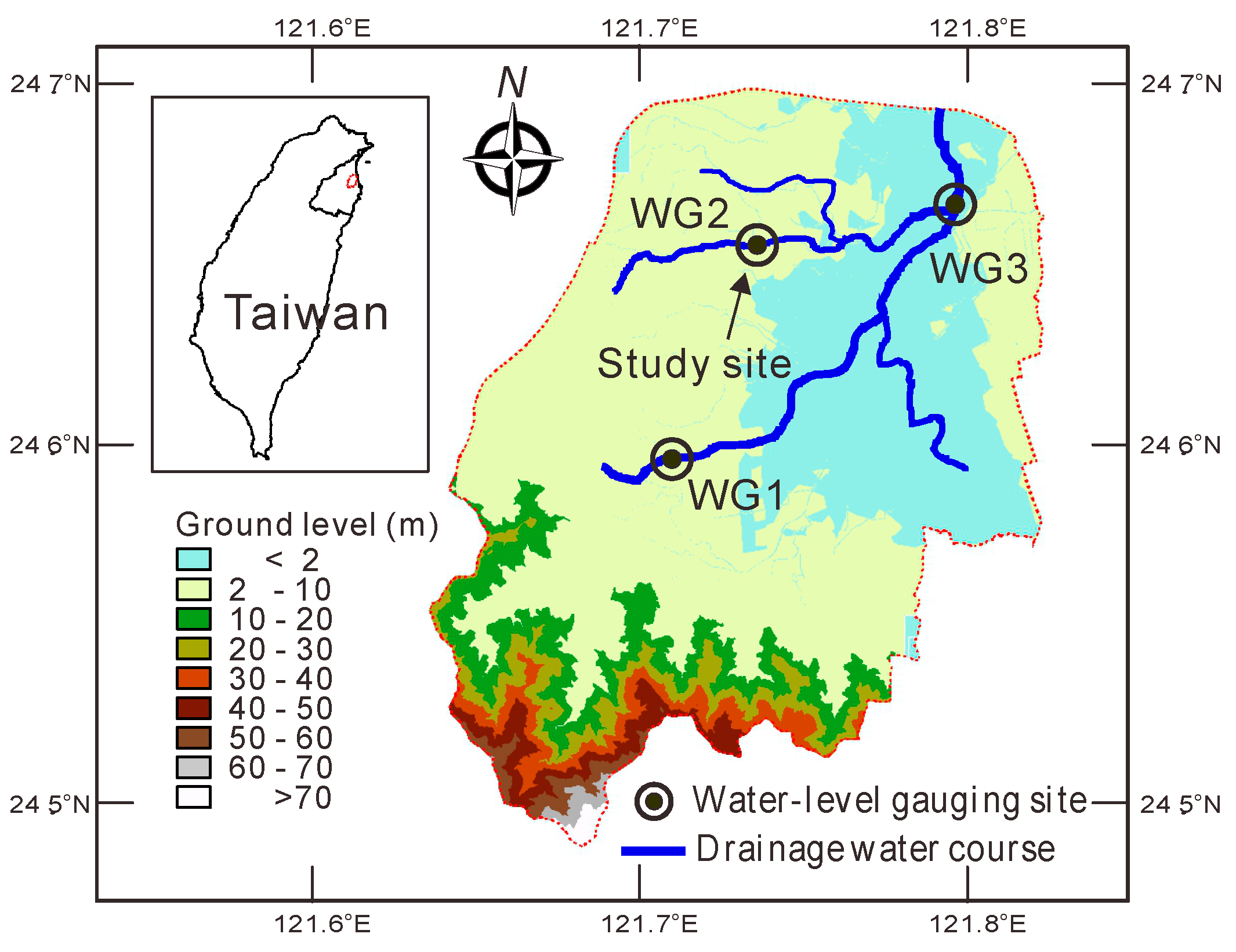
Yilan County (Figure 1), located in northeastern Taiwan, is known for its rainy weather. With about 200 rainy days per year, the annual average precipitation is around 2000–2500 mm. The terrain is surrounded by mountains in the west and coastline in the east. It is frequently hit by typhoons in the summer and autumn of each year. On average, two to three typhoons hit Taiwan every year and among which 45% land in Yilan County [11]. The heavy rainfall during the typhoon attacking period often causes severe inundation in the low-lying areas. Among these inundation-prone areas, the situation in Donsan area (Figure 1) is most extreme. The drainage area of Donsan is about 34 km2. Ground level in the area is very low and flat. The ground elevation in more than one-third of the area is below 2 m, as seen in Figure 1. During typhoon invasion, these low grounds are often flooded, causing heavy damages and tremendous losses to the properties.
The high tendency in severe flooding within the area has raised an urgent need for effective disaster preventive measures. In order to monitor the local inundation condition during the typhoon period, Taiwan Water Resources Agency established a surveillance network for the area in 2011. It includes three water-level gauging stations, as well as a data transmission system that can receive the precipitation observations of the Quantitative Precipitation Estimation and Segregation Using Multiple Sensor (QPESUMS, [12]). QPESUMS consists of eight Doppler radar stations that each scans an area with a radius of approximately 230 km. The system provides quantitative precipitation estimation by integrating observations from weather radars and rainfall readings from 406 automatic gauges and 45 ground stations in Taiwan. QPESUMS also provides rainfall forecasts by tracking and extrapolating the movement paths of storm cells based on radar readings. During the typhoon period, QPESUMS delivers the rainfall data in a frequency of every 10 min through a network connection to the surveillance system. The water level gauging stations return the local inundation water-level data with the same frequency through radio transmission.
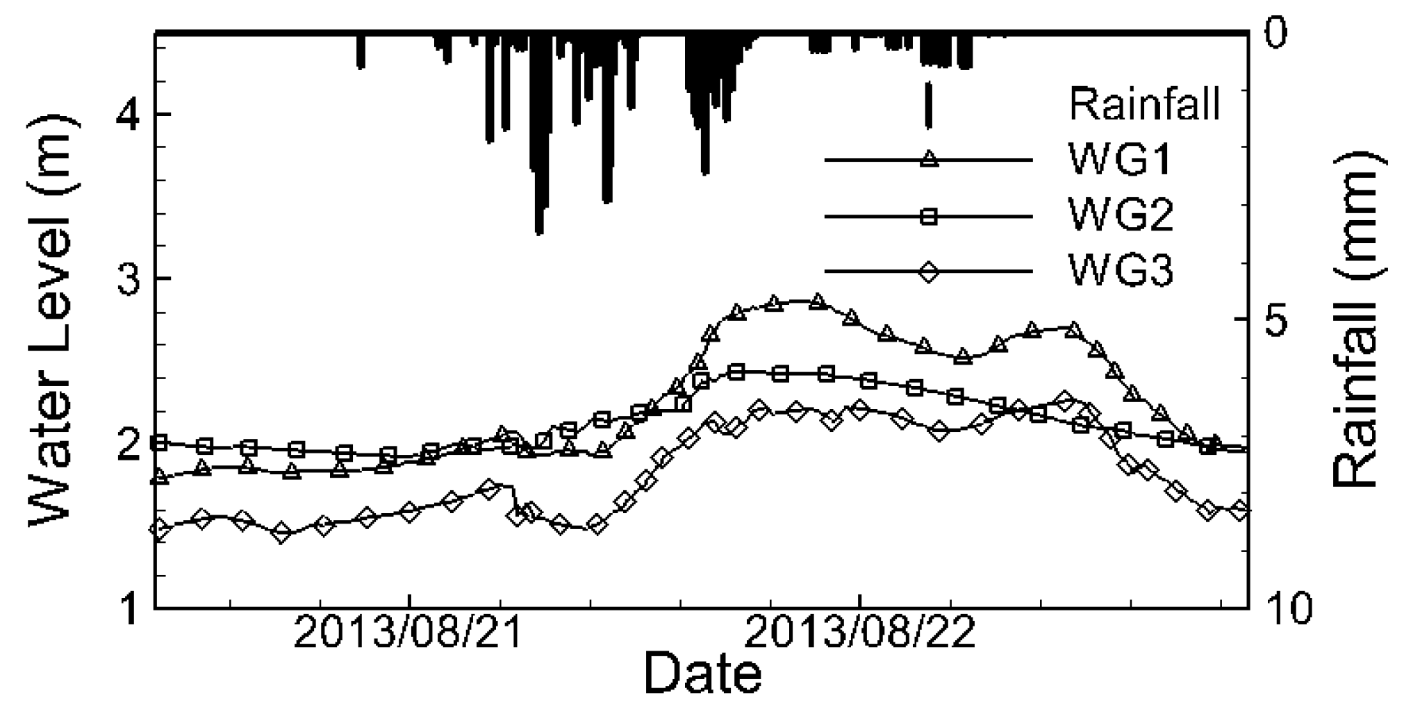
Since the monitoring system of Donsan area was established, it has collected data of 10 typhoons over the years. Figure 2 shows the recorded water level of each station and QPESUMS rainfall data during Typhoon Trami in 2013. Detailed information of each typhoon event is listed in Table 1. These data not only provide the local rainfall and water level information during the typhoon period but can also be used for the establishment of water-level forecast models. In the present study, the WG2 gauging site is selected as the study object to establish the water level forecast model.
2.2. Model Construction
The present study adopts ARX to build the water-level forecast model for the quick calculation feature. ARX is a kind of black-box model which can be divided into the linear model and nonlinear model according to the relationship between the input and output. The nonlinear model can be further subdivided into various types according to the different nonlinear functions applied. The present study respectively aims at linear ARX, as well as ARX with Wavelet function and ARX with Sigmoid function in the nonlinear ARX, to discuss the inundation forecast performance of these three types of models.
With regard to emergency response to the typhoon, the water level is a greater concern than runoff. Therefore, the purpose of the forecast model is to establish the relationship between rainfall and water level, rather than the more commonly seen rainfall and runoff relationship. Although few studies have focused on the relationship between rainfall and water level, relevant works can be found in the literature [13,14,15].
2.2.1. Linear ARX
Linear ARX (LARX) is an extension of the AR model [16] in time series analysis by adding the influence of other exogenous inputs. The equation is as follows:
in which represents the system output; is the exogenous input; and are the number of terms of and , respectively; is the time lag of ; is white noise; through and through are the coefficient of each term, respectively. through and through are called the regressors which take in the known data to forecast . In LARX, the relationship between and the regressors is linear, as shown in Equation (1). In this study, represents the water level at the site of WG2 in Donsan area, while is the local rainfall data provided by QPESUMS.
2.2.2. Nonlinear ARX
Nonlinear ARX extends linear ARX by using a nonlinear relationship between the forecast and the regressors, as shown in the equation below:
where is the nonlinearity estimator which has the following form:
in which is the row vector consists of the regressors, is the number of terms of nonlinearity estimator, and are the coefficients of each term, and is the mean value of the regressor vector. is the nonlinear unit, which can adopt different nonlinear functions.
Two different types of nonlinear ARX models are employed in the present study, viz. the nonlinear ARX with Wavelet function (NLARX-W) and the nonlinear ARX with Sigmoid function (NLARX-S). In NLARX-W, the nonlinear unit adopts the Wavelet function [17], which has the following formula:
where dim represents the dimension of the vector ; is the exponential function.
On the other hand, in NLARX-S, adopts the Sigmoid function as shown in the equation below:
The model structure of LARX, NLARX-W, and NLARX-S is determined by the selection of regressors which are to be determined later on through the optimization process.
2.2.3. Rainfall Data Analysis
To analyze the relationship between water level and rainfall, correlation analysis on typhoon data records was carried out. The definition of the correlation coefficient (CC) is shown below [18]:
in which cov is the covariance between variables and ; and are the standard deviations of and , respectively; is the quantity of the data points. CC ranges between −1 and 1, where −1 represents the perfect negative correlation between and , +1 means the perfect positive correlation, and 0 means that there is no correlation between and .
The rainfall data provided by QPESUMS are 10-min rainfall increments. However, it has been reported by Ouyang [19] that the variation in water level is slower than the variation in rainfall, and often a certain amount of rainfall accumulation is required for the water to build up. To search for the most correlated cumulative rainfall to the water level at the study site, the procedure of Ouyang [19] was adopted here. The moving cumulative rainfall data of the typhoon events with accumulation duration ranging from 1 h to 30 h were first constructed. The correlations of each cumulative rainfall data set and the water level data were then calculated. The results are as shown in Figure 3. The circle dots in the figure represent the average CC of the typhoon events, and the error bars denote the CC distribution of the events. As shown in the figure, the average CC is first gradually increasing along with an increase in the accumulation duration, and then followed by a gradual recession with a further increase in the accumulation duration. As shown in the figure, the maximum average CC appears when the accumulation duration is about 18 h. This indicates that the water level at the study site is most correlated with the 18 h cumulative rainfall which shall be adopted as the input data of the ARX models.
2.2.4. Regressors
The ARX simulation depends on the selection of regressors. With different combinations of regressors, the performance of the model varies. In the selection of model regressors, two methods are commonly utilized in the literature. The first one is Sequential Time Series (see for example, [20,21,22,23]) where a sequence of time series data from the current time to a certain time before is used as model regressors, for example, , , …, , in which represents the cumulative rainfall. The second common method is Pruned Sequential Time Series (see for example [24,25]), which retains only the most relevant period of data sequence as the model input to prevent excessive variables from influencing the model simulations. For example, , …, , where through represent the time period when is most correlated to the water level.
In addition to the above two methods, a third method namely Non-Sequential Time Series has been proposed by Talei et al. [26]. In their study, two antecedent rainfall data and are selected as the model input, in which and are two non-sequential time points determined through a search test. Their results show that the models acquired in this method perform better than those acquired in the two aforementioned methods. In the study of Talei et al. [26], and were determined by a search process using the method of exhaustion. However, this approach of exhaustion search requires tremendous computing resources and CPU time, which makes it only suitable for the combination of a few regressors. The present study improves this aspect by adopting genetic algorithm (GA) for the optimal selection of model regressors, such that the number of model regressors is no longer limited and a vast amount of models with various combinations of regressors can be explored.
In the present study, the input variables of the models are selected non-sequentially from the combination of , , …, , where represents the 18-h cumulative rainfall which, according to the previous data analysis, has been shown most correlated to the water-level. defines the range of regressors to be selected. The greater the value of , the more possible combinations of regressors and thus candidate models can be explored. Considering the computing time required for the search process, is set to be 10 in the present study. The water level forecast is also related to water level data . For simplicity, is also set to be 10 herein. The relation between the regressors and output of each model is summarized below:
in which represents the function of ARX.
2.2.5. Assessing Indexes
In order to search for the optimal models, the following indexes are employed to evaluate the water level forecast capacity of each candidate model.
Coefficient of Efficiency (CE)
CE is an index designed to evaluate the performance of a hydrological model [27]. CE is defined as follows
where and are the observed and estimated water levels, respectively; is the average of observed water level, and is the number of data points. A CE value closer to 1 indicates that the predicted water levels fit more for the observations.
Relative Time Shift Error (RTS)
It has been shown by Talei and Chua [28] that a certain time shift error might emerge when using past data to forecast into the future. The forecasted water-level hydrograph displays a shifted delay in time from the observations. In order to assess the time shift error of the models, the process of Talei and Chua [28] is adopted in this study. The water-level hydrograph predicted by the model is first shifted back in time from 0 to data points, and the CE of each shifted hydrograph is then calculated by comparing to the observations. The shift step associated to the maximum CE is considered as the time shift error of the model. The definition of Relative Time Shift is thus as follows
where denotes the average of the typhoon events, and is the forecast horizon (i.e., prediction time steps; each time step is 10 min in the present study). RTS ranges between 0 and 1. A smaller RTS represents less time shift in the predictions.
Threshold Statistic for a Level of
([29,30]) was employed to assess the error distribution in the forecasted water-level hydrographs. is defined as follows
where is the total amount of data points; is the amount of forecasted data points with absolute relative error less than a specified criteria of . is defined as
where and are the observed and predicted water level at time , respectively; and is the observed water depth. Using water depth instead of water level as the denominator in Equation (11) has several benefits. First, the value of thus defined ranges between 0 and 1, where = 0 indicates perfect prediction and 1 denotes a bad prediction deviated from the observation by the entire water depth. Second, a better accuracy in error measurement is achieved since the scale of water level might be in tens or hundreds of meters (depends on the location where the data were recorded) whereas in water depth it is often in meters only. A greater means that the forecasted water-level hydrograph contains more predicted data points with the absolute relative error less than , and thus the model performance is better. The present study adopts 15% as the threshold value (i.e., ).
2.2.6. Data Processing
The water level and cumulative rainfall data are standardized using the following equation [31]
where is the data after standardization; is the raw data; and are the maximum and minimum of raw data, respectively. The process of data standardization concentrates the dispersive data in a defined interval, which has shown great improvement on the predictions [31].
2.3. Model Optimization
The three indexes of CE, RTS, and each evaluates the model’s water level forecast accuracy, the time shift error, and the error distribution, respectively. All the three indexes provide valuable information for disaster prevention action during typhoon attack and shall be considered at the same time. However, it is difficult to weigh the importance of the three indexes. In order to find the models with good performance in all aspects, the multi-objective genetic algorithm (MOGA) was adopted in the present study as a tool for the search.
2.3.1. Multi-Objective Genetic Algorithm
The theoretical basis of GA was developed based on the Darwinian natural selection theory. After Holland [32] developed a firm mathematical foundation for the algorithm, GA has been widely applied to various fields to solve optimization problems that could not be tackled by traditional methods. In GA, each individual in a population is deemed as a possible solution to the optimization problem at hand. Based on the specified objective functions, the performance of each individual is evaluated and compared, and the individuals with better performance shall have a greater chance to pass its gene to the next generation. Through this procedure, the overall performance of the entire population gradually evolves and improves. After several generations of evolution, the individuals with optimal performance shall emerge, and these optimal individuals are considered as the optimal solutions of the problem. The algorithm has been shown capable of locating the global optima [33] and is particularly suitable for solving multi-objective optimization problems [34].
2.3.2. Objective Functions
Based on the definition of CE, RTS, and , three design goals of the optimal model can be identified, which are the maximum CE, minimum RTS, and maximum , respectively. Also, according to Equations (8)–(10), the upper limit of CE and is 1, and RTS is always a positive number; therefore, the objective functions shall be defined as follows:
in which , , represent the averaged value of the three indexes for the typhoon events, respectively. The design goal of Objective 1 and Objective 3 is to get and closest to 1, while the design goal of Objective 2 is to get closest to 0.
2.3.3. Codification of Regressor Combinations
The design variables of the optimization problem are the various possible combinations of model regressors consisting of through and through , as shown in Equation (7). To utilize MOGA to search for the optimal models, the combination of the regressors has to be codified into a chromosome. In the present study, this procedure is accomplished by using binary bit string codifications, as illustrated in Figure 4. The combination of regressors is represented by a binary bit string chromosome consisting of 22 genes each associated to a specific regressor. If the value of a gene is 1, the regressor associated to this gene shall be selected as an input variable of the model. Contrarily, for a gene with a value of 0, the associated regressor shall not be selected as input. Each chromosome represents a specific combination of regressors and thus a candidate model. With 22 genes in one chromosome, the total candidate models thus formed in the search space are .
For model calibration, 6 out of the 10 events were selected, and the rest events were employed for validation. The selection of the calibration events is based on total cumulative rainfall to represent large, middle, and small amounts of rainfalls. The events thus selected are Songda, Nanmadol, Soulik, Fung-wong, Soudelor, and Dujuan. The three performance indexes of CE, RTS and are calculated and averaged over the validation events. The optimal models for the three types of LARX, NLARX-W, and NLARX-S are searched for using MOGA. With regard to MOGA setting, the population size is set to 200 with Pareto fraction of 0.35. The maximum generation of evolution is 500, and the stopping criterion of the evolution is set to 50 generations of stalls.
3. Results and Discussion
The result acquired by MOGA is the Pareto optimal model set, in which every model is un-dominated, that is, at least one of the three indexes of the model is not exceeded by another model. For each model type of LARX, NLARX-W, and NLARX-S, the three models with the best performance in the three indexes, respectively, are selected among the Pareto optimal set. The results are shown in Table 2. The selected models are named according to their model type and the featuring index, L1 represents the model with the maximum in LARX, L2 represents the one with the minimum in LARX, and L3 represents the maximum model in LARX. Similarly, W1, W2 and W3, as well as S1, S2, and S3, respectively represent the models with the maximum , minimum , and maximum in NLARX-W and NLARX-S. The scores of the nine optimal models on the three indexes and the corresponding chromosomes (i.e., selected regressors) are listed in Table 2. As shown, the selected regressors associated to each of the nine optimal models appear to be in a non-sequential pattern. This supports the result of Talei et al. [26] that a model with non-sequential inputs has better performance than the ones with sequential or pruned sequential inputs.
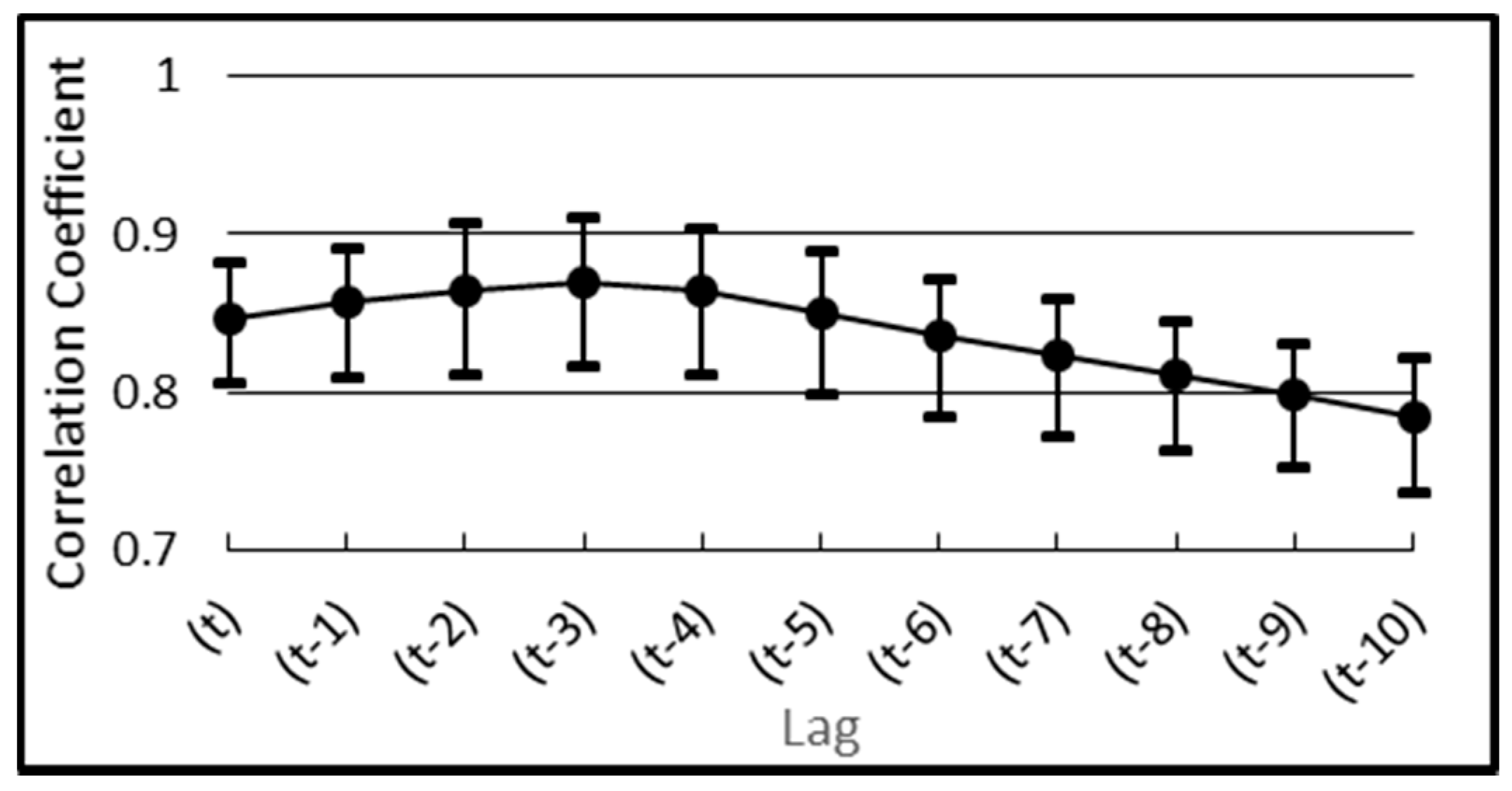
The prediction lead time is crucial for disaster relief action during typhoon attack. An appropriate choice of the prediction lead time has to be linked to the properties of the hydrological behavior of the watershed. It has been observed in the study area that the variation of water level often lags behind the rainfall (for example, as observed in Figure 2). This time lag behavior between the rainfall and the water level presents a characteristic of the watershed, which can be used as an index for the selection of the appropriate prediction lead time. For that, the corrections between the cumulative rainfall data and the water level data shifted back in time by various time lags are analyzed. The results are as shown in Figure 5. The circle dots represent the average CC of the typhoon events and the error bars denote the maximum and the minimum CCs of the events. As seen, the average CC reaches the peak at the time lag of t − 3. This indicates that the water level is most correlated to the cumulative rainfall with 3 h of lead in the study area. The prediction lead time in the present study is thus selected to be 3 h in accordance with this hydrological characteristic of the watershed.
Figure 6a–c compare the performance of the nine models in CE, RTS, and . In the comparison of CE, as shown in Figure 6a, the performance of Model Type 1 (L1, W1, S1) and Model Type 3 (L3, W3, S3) is quite good, in which CE all reaches above 0.8. The CEs of Type 1 Models are seen a little higher than Type 3 Models, but the differences are not significant. The CE performance of Model Type 2 is relatively poorer, especially for L2 and W2. This is because Model Type 2 features on reducing the time shift error. Nevertheless, it is noted that the CE of Model S2 still reaches above 0.7. As shown in Figure 6a, the CEs of the nonlinear models (W- and S-series of models) are somewhat higher than the linear L-series of models, thus indicating that the relationship between rainfall and water level at the site of WG2 is nonlinear. In the comparison of nonlinear models, the CEs of NLARX-S models (S1, S2, S3) appear to be higher than NLARX-W models (W1, W2, W3), and that difference is particularly evident with S2 and W2. In the comparison of time shift errors, as shown in Figure 6b, the RTS of Model Type 2 (L2, W2, S2) is seen lower than Type 1 (L1, W1, S1) and Type 3 (L3, W3, S3). The RTS of S2 in all models is the lowest, showing the minimum time shift error in the forecast, which is followed by W2 with a little increase in RTS; both of which are nonlinear models. The RTS of L2 is the worst in Type 2 models, and as shown in Figure 6b, even W1 and S1 which feature on CE have shown somewhat better performance on RTS than L2. Also, the RTS of the linear L1 and L3 models are much higher than the nonlinear W- and S-series of models. This yet again implies the nonlinearity between the rainfall and the water-level at the study area. Figure 6c is the comparison of the nine models in performance. As shown in the figure, both Type 1 models ((L1, W1, S1) and Type 3 models (L3, W3, S3) display high performance on . Among the nine models, the of S3 is the highest, which is closely followed by W3. The linear L3 has the worst in Type 3 models, which as shown in Figure 6c, is even lower than the nonlinear W1 and S1 that features on CE. In summary, the comparisons in Figure 6 show that the overall performance of nonlinear models is better than linear models on every aspect. Comparisons in the nonlinear models show that the NLARX-S models perform a little better than the NLARX-W models, but the differences are not very significant.
The results of the model predictions might be related to the hydrological behavior of the watershed. As has been shown in Figure 5, the correction between the water level and the rainfall in the study area is most prominent with a time lag of 3 h. It is noted in Table 2 that the model regressors optimized by MOGA all include R(t − 3) in the inputs. This result might reflect the hydrological behavior of the study area. It is also noted that Type 1 and Type 3 models which exhibit higher CE and TS15 values include not only R(t − 3) but also R(t − 4) or R(t − 2) as their regressors. As seen in Figure 2, the correction between the water level and the rainfall in the study area is also high with time lags of t − 2 and t − 4. This might explain the rather good results of CE and TS15 scores achieved by Type 1 and Type 3 models.
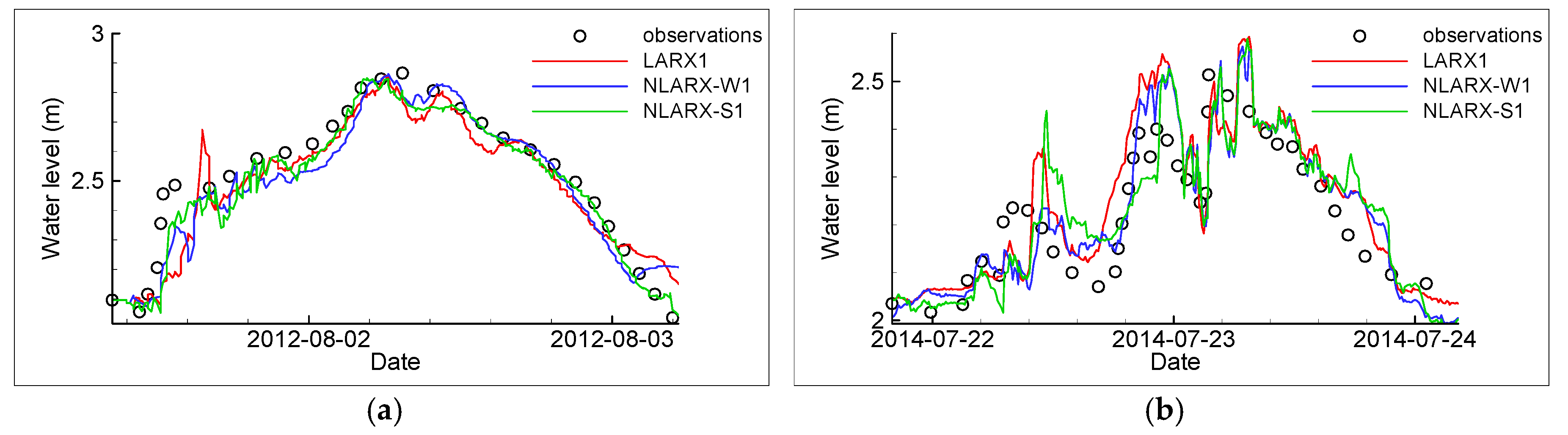
Figure 7 is the comparison of validated water level hydrograph and measured data of Type 1 models, with a prediction lead time of 3 h. Figure 7a–d show the validation results of Typhoon Saola, Matmo, Trami and Usagi, respectively. As seen in the figures, the models generally give reasonable forecasts comparing to the data. It is noted that all the three models exhibit certain degrees of time shift errors on the rising limb of the hydrographs. Since the rising limb of the flood wave is the most important phase for flood forecasting activities, the delayed forecasts pose a limitation of the models.
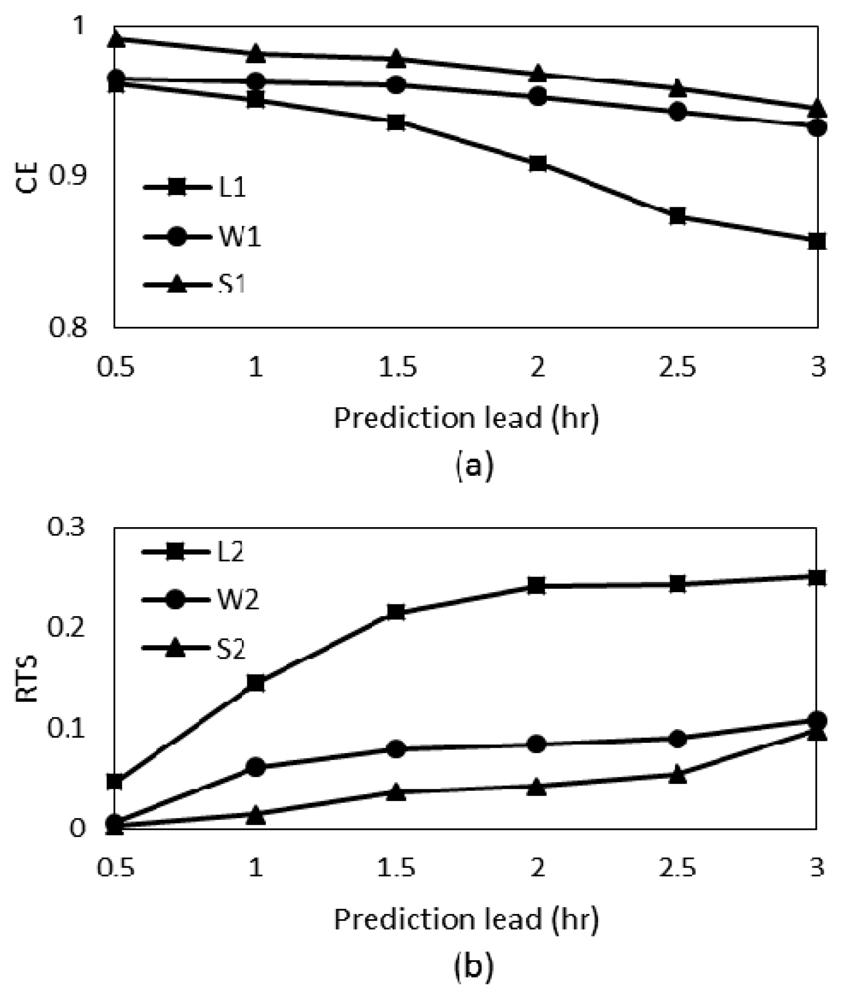
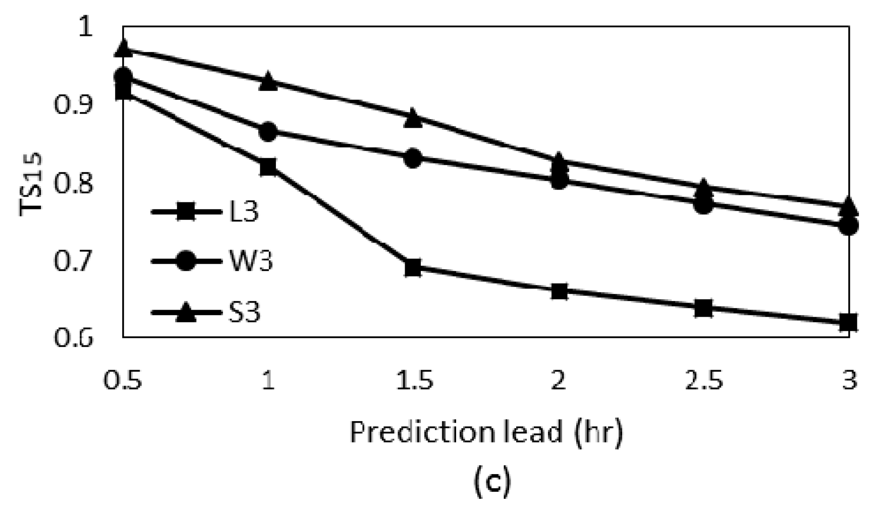
The above model performance comparison is mainly based on 3 h of prediction lead time. In order to investigate the performance under other lead times, the models are applied to the forecasts with prediction lead times varying from 0.5 h to 3 h, and the three indexes of CE, RTS, and associated to each prediction lead time are calculated. The results are shown in Figure 8a–c. Figure 8a shows the CE variations of Type 1 models (L1, W1, and S1) along with the prediction lead. As shown in the figure, it appears that the CEs of all the three models increase with smaller prediction leads. For 0.5 h of prediction lead, the CEs of all models reach above 0.95, among which S1 is the highest. As the prediction lead time increases, the CEs of the three models gradually decrease. CE of L1 drops below 0.9 after the lead time passes 2 h, while W1 and S1 maintain above 0.9 up to 3 h of prediction lead. As the figure shows, for prediction leads from 0.5 to 3 h, CE performance of the three models shows S1 as optimal, closely followed by W1, and L1 is the worst. Figure 8b shows the RTS of Type 2 models (L2, W2, S2) varying along with prediction lead time from 0.5 to 3 h. As shown in the figure, the RTS of the three models gradually increases as the prediction lead time increases. All three models appear to have higher RTS with longer prediction leads, indicating greater relative time shift errors there. Comparing the three models, the RTS performance of S2 appears to be the best, and L2 is the worst. Figure 8c shows the of Type 3 models (L3, W3, S3) varying along with prediction lead time. As shown in the figure, the of all three models increase with smaller prediction leads. With 0.5 h of lead time, of the three models all reach above 0.9, showing very good forecasts. As the prediction lead time increases, the of the three models gradually decreases. The performance of the three models shows S3 as the best, closely followed by W3, and L3 as the worst.
4. Conclusions
A methodology for the determination of the optimal combination of non-sequential regressors for typhoon inundation forecasting models has been developed. By integrating a MOGA with ARX-based models, the proposed methodology is capable of locating the optimal models that conform to multiple objectives in terms of high prediction accuracy, low time shift error, and low threshold statistics. Testing results show that the nine optimal models obtained by the MOGA all display non-sequential patterns in the resultant combinations of regressors, which signifies the superiority of this type of model as well as the capacity of the proposed methodology in locating the optimal non-sequential regressors. In comparing the resultant models obtained by the proposed methodology, the results show that the overall performance of nonlinear models (NLARX-W and NLARX-S) is significantly better than linear models (LARX), revealing a nonlinear relationship between the rainfall and water level at the study area. On all the three assessing indexes of CE, RTS, and , the evaluation results of the three types of models present, in general, NLARX-S as the best, NLARX-W falling slightly behind, and LARX as the worst. These results provide a new approach to constructing better models for typhoon inundation level forecasts.
Acknowledgments
This research was supported by the Ministry of Science and Technology in Taiwan under grant No. MOST 105-2625-M-197-001. Support from the Water Resources Agency in Taiwan is also acknowledged.
Author Contributions
Huei-Tau Ouyang designed the framework of the study; Shang-Shu Shih and Ching-Sen Wu participated in data collection and final approval of the writing.
Conflicts of Interest
The authors declare no conflict of interest.
References
- Karlsson, M.; Yakowitz, S. Rainfall-runoff forecasting methods, old and new. Stoch. Hydrol. Hydraul. 1987, 1, 303–318. [Google Scholar] [CrossRef]
- Liong, S.Y.; Lim, W.H.; Paudyal, G.N. River stage forecasting in Bangladesh: Neural network approach. J. Comput. Civ. Eng. 2000, 14, 1–8. [Google Scholar] [CrossRef]
- Campolo, M.; Soldati, A.; Andreussi, P. Artificial neural network approach to flood forecasting in the River Arno. Hydrol. Sci. J. 2003, 48, 381–398. [Google Scholar] [CrossRef]
- Keskin, M.E.; Taylan, D.; Terzi, O. Adaptive neural-based fuzzy inference system (ANFIS) approach for modeling hydrological time series. Hydrol. Sci. J. 2006, 51, 588–598. [Google Scholar] [CrossRef]
- Shu, C.; Ouarda, T.B.M.J. Regional flood frequency analysis at ungauged sites using the adaptive neuro-fuzzy inference system. J. Hydrol. 2008, 349, 31–43. [Google Scholar] [CrossRef]
- Kia, M.B.; Pirasteh, S.; Pradhan, B.; Mahmud, A.R.; Sulaiman, W.N.A.; Moradi, A. An artificial neural network model for flood simulation using GIS: Johor River Basin, Malaysia. Environ. Earth Sci. 2012, 67, 251–264. [Google Scholar] [CrossRef]
- Lin, G.F.; Lin, H.Y.; Chou, Y.C. Development of a real-time regional-inundation forecasting model for the inundation warning system. J. Hydroinf. 2013, 15, 1391–1407. [Google Scholar] [CrossRef]
- Tehrany, M.S.; Pradhan, B.; Jebur, M.N. Flood susceptibility mapping using a novel ensemble weights-of-evidence and support vector machine models in GIS. J. Hydrol. 2014, 512, 332–343. [Google Scholar] [CrossRef]
- Del Giudice, D.; Reichert, P.; Bareš, V.; Albert, C.; Rieckermann, J. Model bias and complexity–Understanding the effects of structural deficits and input errors on runoff predictions. Environ. Model. Softw. 2015, 64, 205–214. [Google Scholar] [CrossRef]
- Chang, F.J.; Tsai, M.J. A nonlinear spatio-temporal lumping of radar rainfall for modeling multi-step-ahead inflow forecasts by data-driven techniques. J. Hydrol. 2016, 535, 256–269. [Google Scholar] [CrossRef]
- Pan, T.Y.; Chang, L.Y.; Lai, J.S.; Chang, H.K.; Lee, C.S.; Tan, Y.C. Coupling typhoon rainfall forecasting with overland-flow modeling for early warning of inundation. Nat. Hazards 2014, 70, 1763–1793. [Google Scholar] [CrossRef]
- Gourley, J.J.; Maddox, R.A.; Howard, K.W.; Burgess, D.W. An exploratory multisensor technique for quantitative estimation of stratiform rainfall. J. Hydrometeorol. 2002, 3, 166–180. [Google Scholar] [CrossRef]
- Thirumalaiah, K.; Deo, M.C. Real-time flood forecasting using neural networks. Comput. Aided Civ. Infrastruct. Eng. 1998, 13, 101–111. [Google Scholar] [CrossRef]
- Bazartseren, B.; Hildebrandt, G.; Holz, K.P. Short-term water level prediction using neural networks and neuro-fuzzy approach. Neurocomputing 2003, 55, 439–450. [Google Scholar] [CrossRef]
- Yu, P.S.; Chen, S.T.; Chang, I.F. Support vector regression for real-time flood stage forecasting. J. Hydrol. 2006, 328, 704–716. [Google Scholar] [CrossRef]
- Yule, G.U. On a method of investigating periodicities in disturbed series, with special reference to Wolfer’s sunspot numbers. Philos. Trans. R. Soc. Lond. Ser. A Contain. Pap. Math. Phys. Charact. 1927, 226, 267–298. [Google Scholar] [CrossRef]
- Grossmann, A.; Morlet, J. Decomposition of Hardy functions into square integrable wavelets of constant shape. Siam J. Math. Anal. 1984, 15, 723–736. [Google Scholar] [CrossRef]
- Gayen, A.K. The frequency distribution of the product-moment correlation coefficient in random samples of any size drawn from non-normal universes. Biometrika 1951, 38, 219–247. [Google Scholar] [CrossRef] [PubMed]
- Ouyang, H.T. Multi-objective optimization of typhoon inundation forecast models with cross-site structures for a water-level gauging network by integrating ARMAX with a genetic algorithm. Nat. Hazards Earth Syst. Sci. 2016, 16, 1897–1909. [Google Scholar] [CrossRef]
- Furundzic, D. Application example of neural networks for time series analysis: Rainfall–runoff modeling. Signal Process. 1998, 64, 383–396. [Google Scholar] [CrossRef]
- Tokar, A.S.; Markus, M. Precipitation-runoff modeling using artificial neural networks and conceptual models. J. Hydrol. Eng. 2000, 5, 156–161. [Google Scholar] [CrossRef]
- Riad, S.; Mania, J.; Bouchaou, L.; Najjar, Y. Predicting catchment flow in a semi-arid region via an artificial neural network technique. Hydrol. Process. 2004, 18, 2387–2393. [Google Scholar] [CrossRef]
- Chua, L.H.; Wong, T.S.; Sriramula, L.K. Comparison between kinematic wave and artificial neural network models in event-based runoff simulation for an overland plane. J. Hydrol. 2008, 357, 337–348. [Google Scholar] [CrossRef]
- Mitra, S.; Hayashi, Y. Neuro-fuzzy rule generation: Survey in soft computing framework. IEEE Trans. Neural Netw. 2000, 11, 748–768. [Google Scholar] [CrossRef] [PubMed]
- Nayak, P.C.; Sudheer, K.P.; Jain, S.K. Rainfall-runoff modeling through hybrid intelligent system. Water Resour. Res. 2007, 43. [Google Scholar] [CrossRef]
- Talei, A.; Chua, L.H.C.; Wong, T.S. Evaluation of rainfall and discharge inputs used by Adaptive Network-based Fuzzy Inference Systems (ANFIS) in rainfall–runoff modeling. J. Hydrol. 2010, 391, 248–262. [Google Scholar] [CrossRef]
- Nash, J.E.; Sutcliffe, J.V. River flow forecasting through conceptual models part I—A discussion of principles. J. Hydrol. 1970, 10, 282–290. [Google Scholar] [CrossRef]
- Talei, A.; Chua, L.H. Influence of lag time on event-based rainfall–runoff modeling using the data driven approach. J. Hydrol. 2012, 438, 223–233. [Google Scholar] [CrossRef]
- Jain, A.; Ormsbee, L.E. Short-term water demand forecast modeling techniques—Conventional methods versus AI. J. Am. Water Works Assoc. 2012, 94, 64–72. [Google Scholar]
- Jain, A.; Varshney, A.K.; Joshi, U.C. Short-term water demand forecast modeling at IIT Kanpur using artificial neural networks. Water Resour. Manag. 2001, 15, 299–321. [Google Scholar] [CrossRef]
- Rajurkar, M.P.; Kothyari, U.C.; Chaube, U.C. Artificial neural networks for daily rainfall—Runoff modeling. Hydrol. Sci. J. 2002, 47, 865–877. [Google Scholar] [CrossRef]
- Holland, J.H. Genetic algorithms and the optimal allocation of trials. SIAM J. Comput. 1973, 2, 88–105. [Google Scholar] [CrossRef]
- Goldberg, D.E.; Holland, J.H. Genetic algorithms and machine learning. Mach. Learn. 1988, 3, 95–99. [Google Scholar] [CrossRef]
- Bagchi, T.P. Multi-Objective Scheduling by Genetic Algorithms; Springer Science & Business Media: New York, NY, USA, 1999; pp. 143–145. [Google Scholar]
Figure 1.
Donsan area in Yilan County, Taiwan.

Figure 2.
Water level and rainfall records during Typhoon Trami in Donsan area, Taiwan.

Figure 3.
Correlations between water level and cumulative rainfall with various accumulation durations.
Figure 3.
Correlations between water level and cumulative rainfall with various accumulation durations.
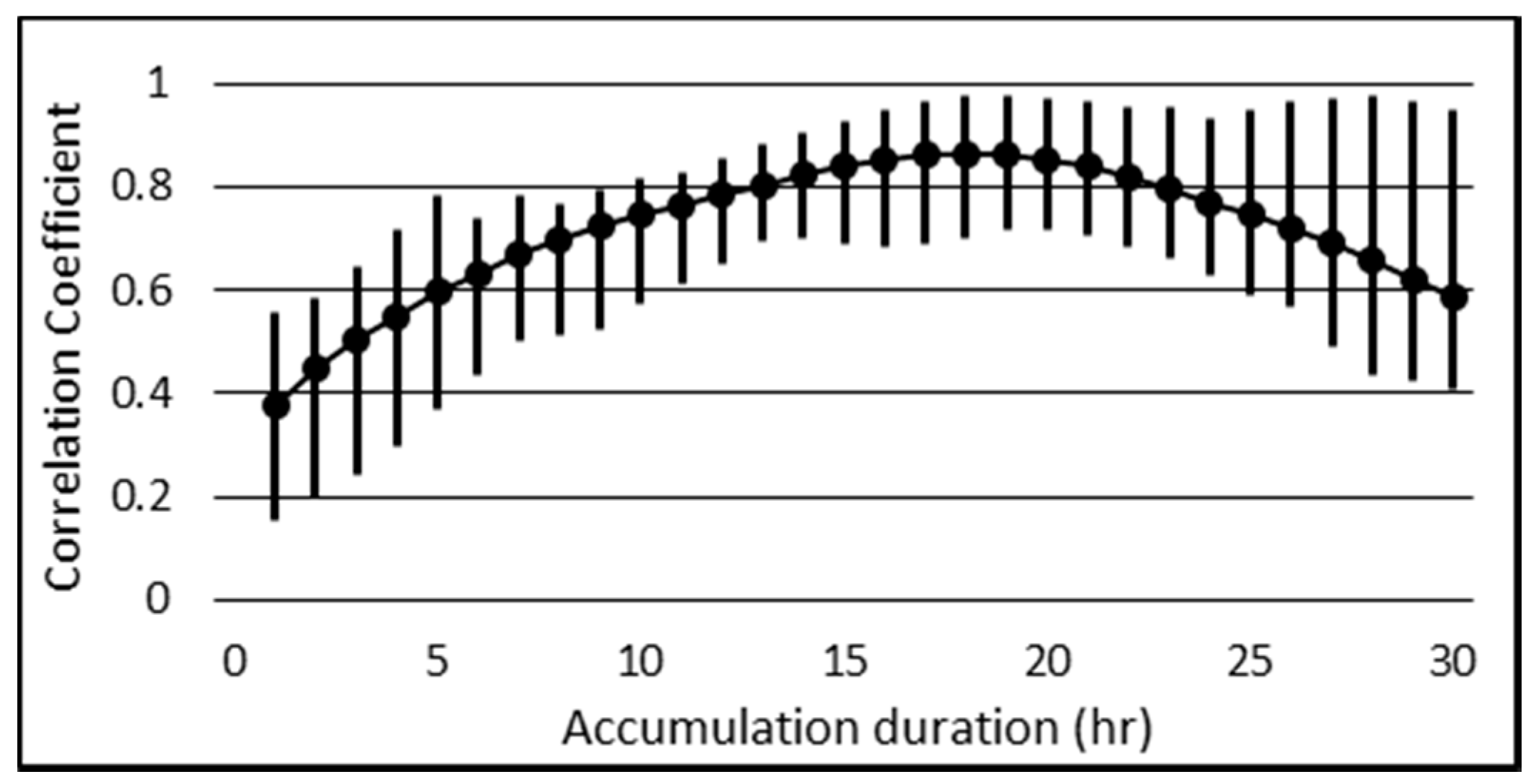
Figure 4.
Binary bit string codification of a combination of regressors.
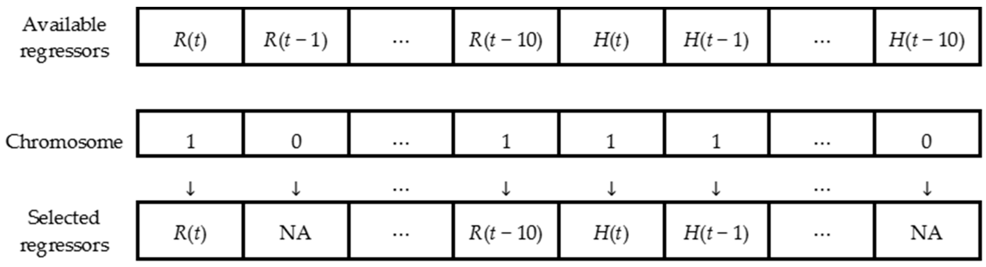
Figure 5.
Correlations between cumulative rainfall and water level with various time lags.

Figure 6.
Performance comparison of the optimal models (a) Coefficient of efficiency (CE), (b) Relative time shift error (RTS) and (c) Threshold statistic for a level of .
Figure 6.
Performance comparison of the optimal models (a) Coefficient of efficiency (CE), (b) Relative time shift error (RTS) and (c) Threshold statistic for a level of .
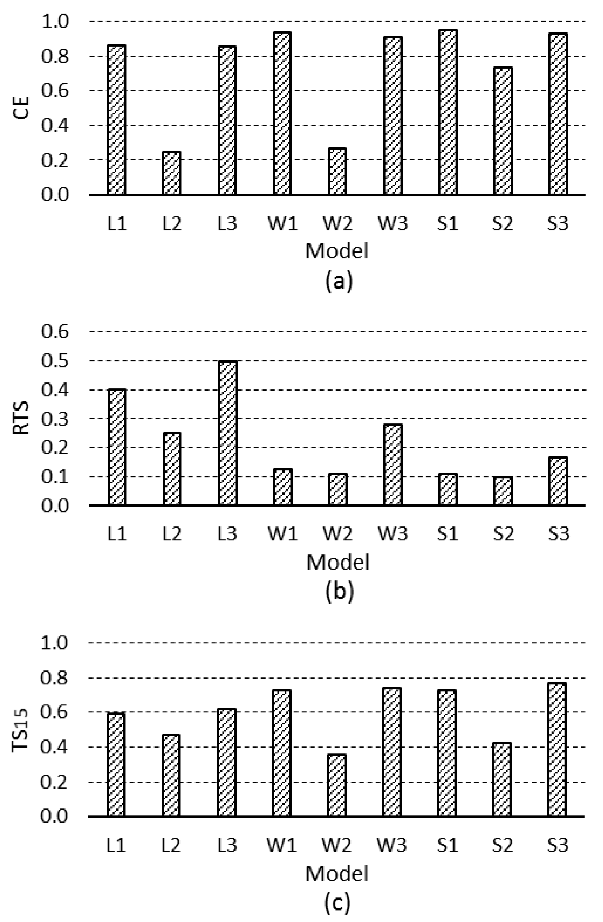
Figure 7.
Comparison of model validation and measured data for (a) Typhoon Saola, (b) Typhoon Matmo, (c) Typhoon Trami, and (d) Typhoon Usagi (3-h lead time).
Figure 7.
Comparison of model validation and measured data for (a) Typhoon Saola, (b) Typhoon Matmo, (c) Typhoon Trami, and (d) Typhoon Usagi (3-h lead time).

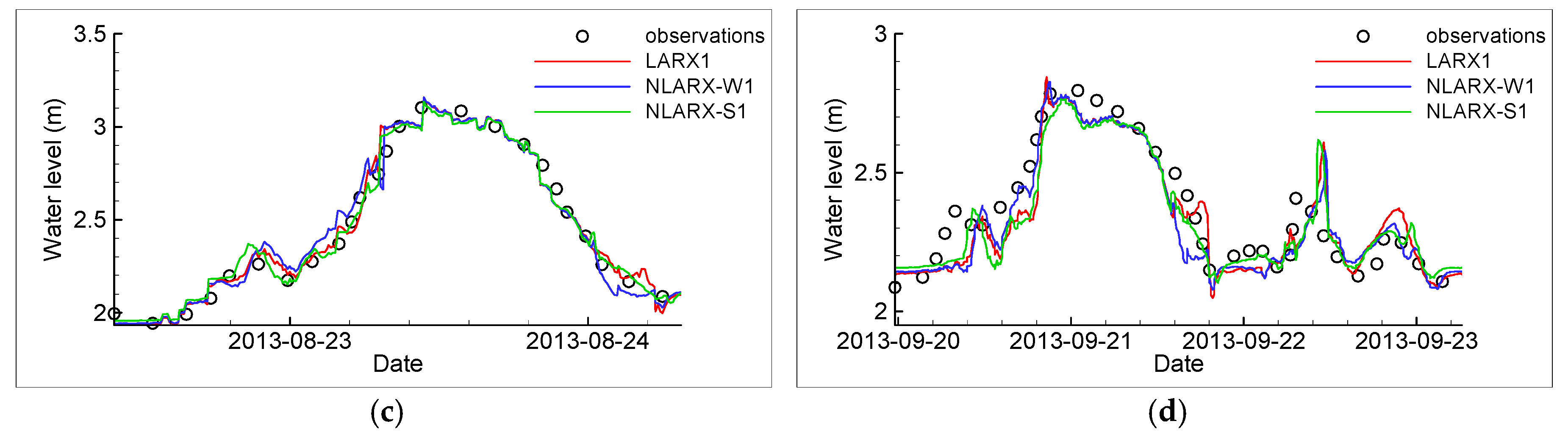
Figure 8.
Variation of assessing indexes of the optimal models with respect to different prediction lead times (a) CE, (b) RTS and (c) TS15.
Figure 8.
Variation of assessing indexes of the optimal models with respect to different prediction lead times (a) CE, (b) RTS and (c) TS15.


Table 1.
Historical typhoon records in Donsan area.
| Typhoon | Year | Time of Official Typhoon Sea Warning Issued h/Day/Month (UTC) | Affecting Period (h) | Maximum Rainfall Intensity (mm/h) | Cumulative Rainfall (mm) |
|---|---|---|---|---|---|
| Songda | 2011 | 0230/27/May | 36 | 28.5 | 213 |
| Nanmadol | 2011 | 0530/27/August | 99 | 26.5 | 172 |
| Saola | 2012 | 2030/30/July | 90 | 37.5 | 537 |
| Soulik | 2013 | 0830/11/July | 63 | 30.0 | 133 |
| Trami | 2013 | 1130/20/August | 45 | 22.0 | 461 |
| Usagi | 2013 | 2330/20/September | 93 | 23.0 | 165 |
| Matmo | 2014 | 1730/21/July | 54 | 35.5 | 98 |
| Fung-wong | 2014 | 0830/19/September | 72 | 41.0 | 72 |
| Soudelor | 2015 | 1130/6/August | 69 | 87.5 | 421 |
| Dujuan | 2015 | 0830/27/September | 57 | 42.0 | 218 |
Table 2.
Optimal models and the corresponding chromosomes (L1–L3: optimal Linear Auto-Regressive model with eXogenous inputs (LARX) models; W1–W3: optimal nonlinear ARX with Wavelet function (NLARX-W) models; S1–S3: optimal nonlinear ARX with Sigmoid function (NLARX-S) models; R(t − 1) through R(t − 10): antecedent cumulative rainfall data; H(t − 1) through H(t − 10): antecedent water level data).
| Index | Model | ||||||||
|---|---|---|---|---|---|---|---|---|---|
| L1 | L2 | L3 | W1 | W2 | W3 | S1 | S2 | S3 | |
| CE | 0.859 | 0.245 | 0.852 | 0.933 | 0.269 | 0.911 | 0.946 | 0.734 | 0.929 |
| RTS | 0.403 | 0.251 | 0.500 | 0.125 | 0.108 | 0.278 | 0.111 | 0.098 | 0.167 |
| TS15 | 0.590 | 0.472 | 0.618 | 0.728 | 0.356 | 0.743 | 0.725 | 0.426 | 0.768 |
| Available regressor | Chromosome (Selected regressor) | ||||||||
| R(t − 1) | 1 | 0 | 0 | 0 | 0 | 0 | 1 | 1 | 1 |
| R(t − 2) | 0 | 0 | 1 | 0 | 0 | 0 | 1 | 0 | 0 |
| R(t − 3) | 1 | 1 | 1 | 1 | 1 | 1 | 1 | 1 | 1 |
| R(t − 4) | 1 | 0 | 1 | 1 | 0 | 1 | 1 | 0 | 1 |
| R(t − 5) | 0 | 0 | 0 | 0 | 0 | 0 | 1 | 1 | 1 |
| R(t − 6) | 1 | 1 | 0 | 0 | 0 | 0 | 0 | 1 | 1 |
| R(t − 7) | 0 | 0 | 0 | 0 | 0 | 0 | 1 | 0 | 0 |
| R(t − 8) | 0 | 0 | 0 | 1 | 0 | 1 | 1 | 1 | 1 |
| R(t − 9) | 0 | 0 | 0 | 0 | 0 | 0 | 0 | 1 | 1 |
| R(t − 10) | 0 | 0 | 0 | 0 | 0 | 0 | 1 | 1 | 1 |
| H(t − 1) | 0 | 0 | 1 | 0 | 0 | 0 | 0 | 0 | 0 |
| H(t − 2) | 0 | 1 | 0 | 0 | 1 | 1 | 0 | 0 | 1 |
| H(t − 3) | 0 | 0 | 0 | 0 | 1 | 0 | 1 | 0 | 0 |
| H(t − 4) | 0 | 1 | 0 | 0 | 1 | 0 | 0 | 0 | 0 |
| H(t − 5) | 1 | 0 | 0 | 0 | 0 | 0 | 0 | 0 | 0 |
| H(t − 6) | 0 | 0 | 1 | 0 | 0 | 0 | 0 | 1 | 0 |
| H(t − 7) | 0 | 1 | 0 | 0 | 0 | 0 | 0 | 0 | 0 |
| H(t − 8) | 0 | 1 | 0 | 1 | 0 | 0 | 0 | 1 | 0 |
| H(t − 9) | 0 | 0 | 0 | 0 | 1 | 0 | 0 | 0 | 1 |
| H(t − 10) | 0 | 0 | 0 | 0 | 0 | 0 | 0 | 0 | 0 |
| Prediction lead: k = 18 (3 h) | |||||||||
© 2017 by the authors. Licensee MDPI, Basel, Switzerland. This article is an open access article distributed under the terms and conditions of the Creative Commons Attribution (CC BY) license (http://creativecommons.org/licenses/by/4.0/).
Share and Cite
MDPI and ACS Style
Ouyang, H.-T.; Shih, S.-S.; Wu, C.-S. Optimal Combinations of Non-Sequential Regressors for ARX-Based Typhoon Inundation Forecast Models Considering Multiple Objectives. Water 2017, 9, 519. https://doi.org/10.3390/w9070519
AMA Style
Ouyang H-T, Shih S-S, Wu C-S. Optimal Combinations of Non-Sequential Regressors for ARX-Based Typhoon Inundation Forecast Models Considering Multiple Objectives. Water. 2017; 9(7):519. https://doi.org/10.3390/w9070519
Chicago/Turabian StyleOuyang, Huei-Tau, Shang-Shu Shih, and Ching-Sen Wu. 2017. "Optimal Combinations of Non-Sequential Regressors for ARX-Based Typhoon Inundation Forecast Models Considering Multiple Objectives" Water 9, no. 7: 519. https://doi.org/10.3390/w9070519
Note that from the first issue of 2016, this journal uses article numbers instead of page numbers. See further details here.