Quantifying Spatial Changes in the Structure of Water Quality Constituents in a Large Prairie River within Two Frameworks of a Water Quality Model

Abstract

A global sensitivity analysis was carried out on a water quality model to quantify the spatial changes in parameter sensitivity of a model of a large prairie river, the South Saskatchewan River (SSR). The method is used to assess the relative impacts of major nutrient loading sources and a reservoir on the river’s water quality. The river completely freezes over during winter; hence, the sensitivity analysis was carried out seasonally, for winter and summer, to account for the influence of ice-covered conditions on nutrient transformations. Furthermore, the integrity of the river’s aquatic ecosystem was examined through the inter-relationship between variables and comparing hierarchy index values and water quality indices at four locations along the river. Sensitivities of model parameters varied slightly at different locations along the river, with the phytoplankton growth rate being the most influential parameter. Nitrogen and phosphorus transformation processes were more sensitive in winter, while chlorophyll-a and dissolved oxygen parameters showed higher sensitivity in summer. A more complicated correlation between variables was observed downstream of the junction of the Red Deer River. Our results reveal that the lower correlation between variables may suggest a more balanced and healthier system, although further analysis is needed to support this statement.

1. Introduction

Increased nutrient loads in rivers and reservoirs lead to eutrophication and, in turn, degrade the surface waters’ ecosystem health [1,2]. High nutrient enrichment can lead to major health issues in aquatic ecosystems, with the most common concern being excessive algal blooms [2]. Monitoring nutrients and quantifying water quality conditions of surface waters are both vital when attempting to manage eutrophication. Utilizing measured data alone is often not informative enough for making water management decisions, due to the resolution coarseness of spatial and temporal data [3]. Thus, water quality modeling and theoretical analysis are essential for water quality management [2,3]. A wide variety of surface water quality modeling studies have been undertaken to estimate nutrient concentrations in waterbodies. However, only a few modeling studies have been carried out on surface waters under ice conditions. Ice covers affect the hydrology and the biological and chemical conditions of rivers, particularly evident in changes in dissolved oxygen concentrations [4,5].

The water quality analysis was augmented with sensitivity and uncertainty analyses to evaluate the model’s behavior and identify dependencies within the model structure [6,7,8,9]. A variety of techniques exist for sensitivity analysis, including local sensitivity andglobal sensitivity [6,7,8,9,10]. Reusser and Zehe [11] proposed a temporal sensitivity analysis method to detect the periods of poor model performance and the dominant parameters. This temporal error analysis helped to better understand the model structure and its deficits [11,12,13]. Lindenschmidt & Chun [14] carried out a global sensitivity analysis (GSA) to assess the impact of fluvial geomorphology on river ice cover formation. They used GSA to highlight important processes, identify sensitive regions within the parameter space, and investigate the strength of the interactions between parameters and variables.

There are several water quality models to quantify the substance transformations in river and streams, such as QUAL2E [15], QUAL2K [16], WASP7 [17], CE-QUAL-RIV1 [18], and SWAT [19,20]. There are also several studies conducting sensitivity analysis with different water quality models to investigate the sensitivity of water quality variables to different parameters. Examples include the work of Drolc and Koncan [21], who studied parameter sensitivity to dissolved oxygen using the QUAL2E model and the work of Griensven et al. [22] that used SWAT to examine parameter sensitivity to water quality variables. In this study, we used WASP (Water Quality Analysis Simulation Program) [17], which has been widely used to assess the water quality of various waterbodies such as lakes, rivers, and estuaries (e.g., Franceschini & Tsai [23], Kaufman [24], Lindenschmidt [25]). The latest version, WASP7, accounts for ice-covered conditions and was selected for this study to predict algal-nutrient dynamics along the South Saskatchewan River (SSR), both in summer and under ice-covered conditions in winter.

The main objective of this paper is to determine the spatial changes of the sensitivity of different water quality variables to various parameters. The determination of such spatial changes is of significance to understand the impact of nutrient loading from tributaries and effluents from lagoons and wastewater treatment plants on different water quality variables along a river. It also helps to understand the impact of lakes and reservoirs on water quality along the river, as reportedly they increase retention of nutrients through increased deposition [26,27]. Therefore, GSA was used to examine the potential impact of nutrient loading point sources (the RDR and effluents from the Saskatoon wastewater treatment plant) and the retention capacity of Lake Diefenbaker. Seasonality of parameter sensitivity is also taken into account to examine the effect of ice-covered conditions. Furthermore, this study examines the correlation between parameters and state variables and their interactions with water quality at four water quality stations along the river.

2. Methods

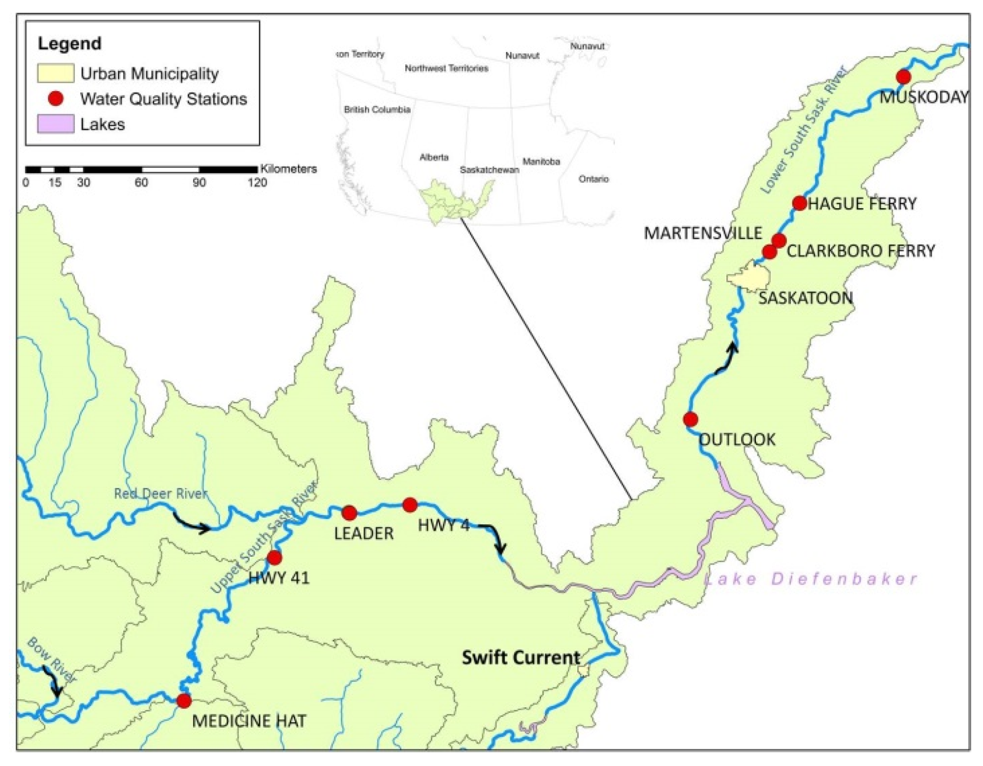
2.1. Site Description

The SSR originates at the confluence of the Bow and Oldman rivers in Alberta, Canada, flows into south-central Saskatchewan and joins with the North Saskatchewan River to flow onward as the Saskatchewan River. Lake Diefenbaker, a reservoir formed by the construction of the Gardiner and Qu’Appelle River dams, modulates the flow of the SSR to secure water for domestic, agricultural and municipal water supplies, provides flood protection and hydropower supply, and maintains aquatic and riparian ecosystems.

The SSR was divided into two major modeling domains:

• upper SSR (uSSR), originating at the confluence of Bow and Oldman rivers to the inlet of Lake Diefenbaker.
• lower SSR (lSSR), originating at the Gardiner Dam and extending to the confluence of the North and South Saskatchewan rivers at the Saskatchewan River Forks east of Prince Albert.

The RDR is a major tributary of the upper South Saskatchewan River and provides forty percent of the flow to the uSSR. The RDR is a nutrient-rich river, with a large amount of phosphorus originating from intensive agricultural activities [28] Rapid agricultural and population growth has elevated nutrient loading into the river, making monitoring and management of surface water quality more pertinent [28].

Lake Diefenbaker is the only reservoir along the SSR that receives a high amount of phosphorus from the uSSR inflow (3146 t TP/yr). The trophic level is classified as meso to eutrophic at the inlet [29,30]. Due to sediment deposition and phosphorus retention in the lake, the water quality improves downstream of the Gardiner and Qu’Appelle dam arms, where the water quality is classified as oligo to mesotrophic [30,31]. The SSR receives large lagoon effluents and treated effluent from the Saskatoon wastewater treatment plant.

To study the impact of Lake Diefenbaker and the nutrient loads from the RDR and Saskatoon wastewater treatment plant, four stations along the SSR were selected: Medicine Hat, Leader, Outlook, and Clarkboro Ferry. The locations of these sites are shown in Figure 1.

Figure 2 compares the measured concentrations of total nitrogen (TN), total phosphorus (TP), dissolved oxygen (DO), and chlorophyll-a (CHLA) at the selected stations along the SSR. Higher concentrations of TP, DO, and CHLA, but lower TN concentrations, were observed in the uSSR downstream of the RDR inlet. As reported earlier, Lake Diefenbaker is an efficient phosphorus trap and the measured concentrations show a reduction in the TP and CHLA concentrations between the inlet and outlet of the lake (difference between “b” and “c” in Figure 2). However, surprisingly, several algal bloom events were recorded in the Qu’Appelle Dam arm of Lake Diefenbaker [26] and at Outlook (difference between “c” and “d” in Figure 2). Lower CHLA and higher TN were observed in the lSSR after receiving effluents from Saskatoon.

A seasonal trend was observed for the water quality of the SSR. As Figure 2 shows, DO and nitrate (NO3) concentrations are higher in winter than in summer. CHLA and TP concentrations are typically higher in summer compared to winter.

The measured forcing data during the study period included daily flow, water temperature, and daily solar radiation and are presented as supplementary materials in Section A.

2.2. Model Description and Set-up

The eutrophication module in the Water Quality Analysis Simulation Program (WASP7) was used to model water quality of the SSR. WASP7 is an enhanced MS Windows version of the original program that was developed by the U.S. Environmental Protection Agency [17,32,33]. The model is continually extended and updated and has a user-friendly interface that allows ease of applicability and facilitates learning in an educational environment. Additionally, the model can be run in batch mode for sensitivity and uncertainty analysis within a Monte-Carlo framework. Therefore, for this study, the WASP model was selected in lieu of other compatible water quality models such as CE-QUAL-RIV1. The eutrophication module uses a series of mass balance equations to simulate the spatial and temporal transport and transformation of nutrients, phytoplankton, and dissolved oxygen in the aquatic environment. The variables studied in this paper are phytoplankton carbon represented by chlorophyll-a (CHLA), ammonium (NH4), nitrate (NO3), dissolved oxygen (DO), organic nitrogen (ON), organic phosphorus (OP) and orthophosphate (OPO4).

In this study, we used two WASP7-based water quality models already developed and calibrated by Akomeah et al. [34] and Hosseini et al. [35] for the upper and lower parts of the SSR, respectively. They calibrated these models using a trial-and-error approach to achieve an acceptable model performance with respect to measured values. They also validated their models with independent datasets (yielded r² values of 0.69 for the lSSR, and 0.68 and 0.94 for the uSSR at Leader and Medicine-Hat), demonstrating the predictability of the developed models to describe our river system. In the present study, we utilized these established water quality models to carry out a global sensitivity analysis to assess the strength of the interactions between water quality parameters and state variables. The sensitivity results were compared at four different locations to investigate the effect of the RDR, Lake Diefenbaker, and effluents of the Saskatoon wastewater treatment plant on the water quality of the river.

The setup for each model, for the uSSR and the lSSR, is briefly explained in this section, but more details of the model descriptions can be found in Akomeah [34] and Hosseini [35]. The river was discretized horizontally along the longitudinal profile of the river. The uSSR is about 476 km long and was discretized using 693 segments, each 700 m long. Similarly, the 330-km long lSSR was divided into 673 segments, each 500 m in length. Morphological characteristics of the segments were estimated based on surveyed cross-sectional profiles. The boundary conditions were estimated from the nearest water quality sampling stations and are provided in the supplementary materials, Section B. The initial concentration conditions in segments were calculated by averaging and interpolating water quality concentrations between two adjacent sampling stations.

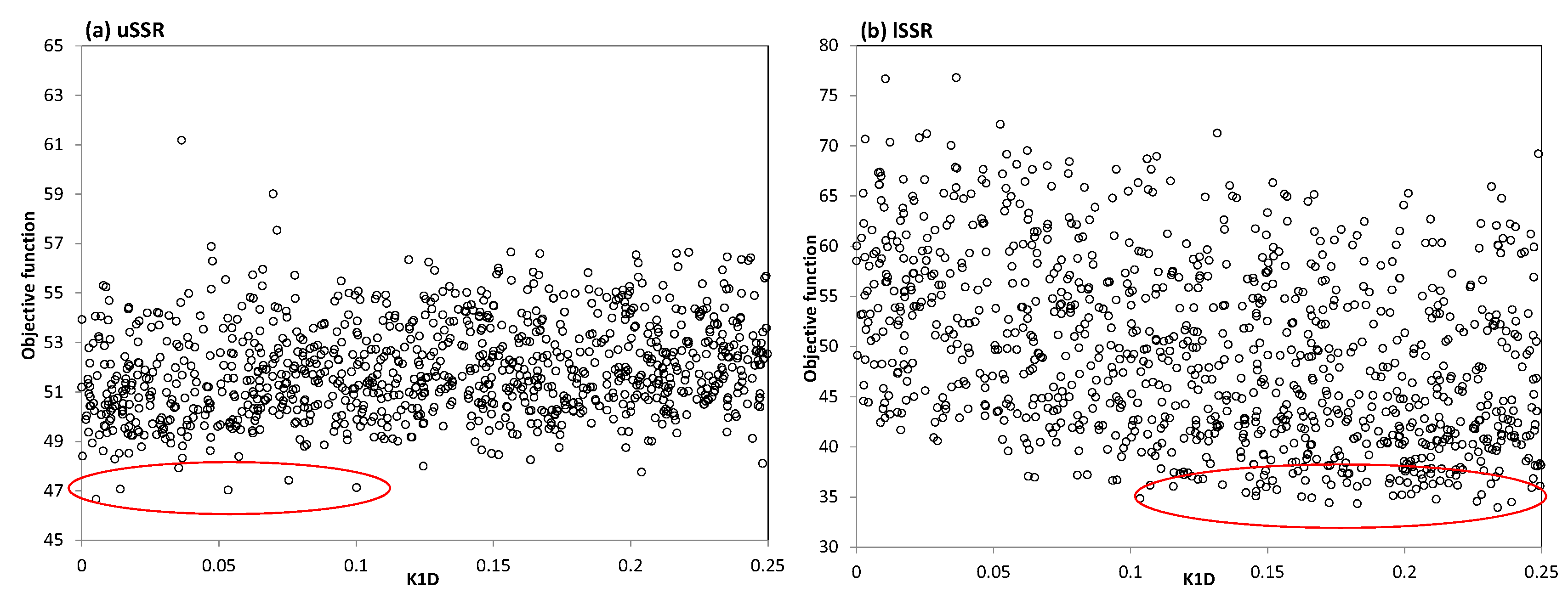
2.3. Parameter Sensitivity

A GSA was conducted to study the effect of parameters on model output within their entire parameter space and to identify the interactions between parameters. Various approaches to sensitivity analysis have been used in the literature, including simple one-factor-at-a-time strategies [36], Monte-Carlo filtering [37], variance-based approaches [38], and a variogram-based framework [39,40]. In this study, a Monte-Carlo Analysis (MOCA) framework was used with many model simulations, each using a different set of parameter values sampled randomly from a certain range of model parameters. For each simulation, the parameters were randomly generated from uniform distributions within the parameter ranges, which for the most part, were derived from the literature and the WASP7 model manual. The initial parameter settings are those calibrated from Akomeah [34] and Hosseini [35] and are listed in

Table 1. Selected parameters for sensitivity analysis.

Parameter Description	Parameter (Unit)	Ranges	Initial Values
			uSSR	lSSR
Nitrification rate	K12C (1/day)	0–3	0.1	2
Denitrification rate	K20C (1/day)	0–0.09	0.05	0.01
Phytoplankton growth	K1C (1/day)	0–3	0.6	0.5
Carbon to Chlorophyll-a ratio	CCHL (mgC/mgChla)	20–60	30	40
Phytoplankton death rate	K1D (1/day)	0–0.25	0	0.2
1/2 saturation for N-limitation	KMNG1 (mg N/L)	0–0.05	0.02	0.03
1/2 saturation for P-limitation	KMPG1 (mg P/L)	0–0.05	0	0.03
Nitrogen to Carbon ratio	NCRB (mg N/mg C)	0–0.43	0.15	0.1
Phosphorus to Carbon ratio	PCRB (mg P/mg C)	0–0.24	0	0.15
TON mineralization rate	K71C (1/day)	0–1.08	0.075	0.075
TOP mineralization rate	K83C (1/day)	0–0.22	0.02	0.22
Fraction of phyto. death recycled to ON	fON	0–1	0.5	0.8
Fraction of phyto. death recycled to OP	fOP	0–1	1	0.8
Sediment Oxygen Demand	SOD (g/m2/day)	0–0.5	0.5	0.5
Reaeration in winter	K2w (1/day)	0–0.5	1.4 *	0.1
Reaeration in summer	K2s (1/day)	1–3	1.4	1.5

* In Akomeah, et al., [34] the reaeration rate was defined as 1.4 (1/day) for the entire simulation period.

.

To run the model automatically, the WASP7 model was linked to OSTRICH (Optimization Software Tool for Research In Computational Heuristics), an open-source and model-independent code that can automate the processes of model calibration and evaluation [41].

In this study, we conducted two analyses to assess (1) the sensitivity of “individual” model variables to model parameters, and (2) the “overall” (collective) sensitivity of the model response (based on the entire model variables) to model parameters and their interactions. For the first analysis, the simulation performance for each variable was based on the sum of squared errors between simulated and observed values. To evaluate the sensitivity of overall model response to the parameters, the sum of normalized square errors (SNSE) was used, as shown in Equation (1):

$$\text{SNSE}={\displaystyle \sum }_{j=1}^n{\displaystyle \sum }_{i=1}^k{(\frac{C_{sim}(i,j)-C_{obs}(i,j)}{{\overline{C}}_{obs}(j)})}^2$$

(1)

where n is the number of variables and k is the number of observations considered for sensitivity analysis. C_sim(i.j), C_obs(i,j)_, and ${\overline{C}}_{obs}(j)$ are simulated, observed and mean observed values for each variable, respectively.

In both of the analyses described above, those parameter sets yielding good or poor performing simulation results were classified respectively as behavioral and non-behavioral [42]. The behavioral sets were deemed to be those simulations yielding the best 10% of the simulated output. The cumulative distributions of the behavioral parameters were compared to the cumulative distributions of the entire parameter sets (i.e., a priori parameter sets). The parameter with greater deviation between the two curves is deemed to have the greater (most sensitive) impact on the model output. The Kolmogorov–Smirnov test was used to quantify the distance between the cumulative distributions of the behavioral parameters of the a priori parameter sets. The parameter sensitivity was classified using the significance level (α) of differences between the behavioral and a priori distributions. The significance level is the level at which the null hypothesis, that the two distributions are the same, is accepted. The same top 10% of the parameter sets were used to examine the interactions between parameters and to generate correlation maps.

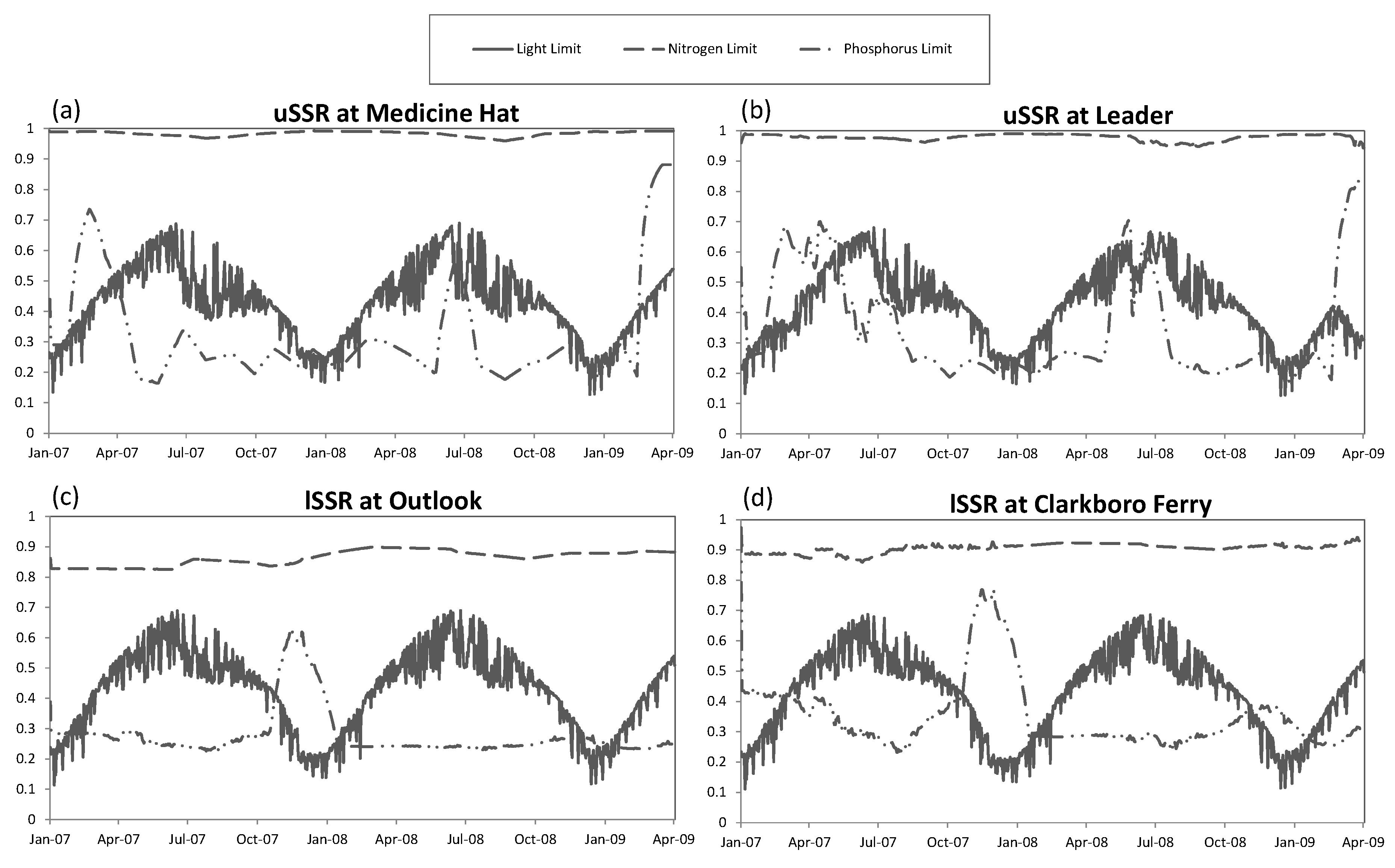
2.4. Nutrient and Light Limitations

Light and nutrients are the most important resources for phytoplankton growth. Phytoplankton growth will be limited under the conditions of light deficiency or inadequate amount of nutrients relative to each other. Determining the limiting factor is important for watershed management and eutrophication control approaches [3,43,44]. Light limitation is a function of solar radiation, fraction of daylight, depth of the water column, and total light extinction. In WASP7, the limitation factors are calculated using the following equations:

$${\varphi }_L=\frac{e}{K_{e}D}f\left[\exp \left\{-\frac{I_a}{I_s}\exp (-K_{e}D)\right\}-\exp \left(-\frac{I_a}{I_s}\right)\right]$$

(2)

• ɸ_L = light limitation factor
• $I_a$= the average incident light intensity during daylight hours below the surface, (ly/day)
• $I_s$= the saturating light intensity of phytoplankton, (ly/day)
• K_e = the light extinction coefficient, (m⁻¹)
• D = depth of the water column or model segment, (m)
• f = fraction day that is daylight, (unitless)

Nutrient limitation is a function of dissolved inorganic phosphorus or nitrogen and varies between 0 (complete limitation) and 1 (no limitation).

$${\varphi }_N=Min\left(\frac{DIN}{K_{mN}+DIN},\frac{DIP}{K_{mP}+DIP}\right)$$

(3)

• ɸ_N = nutrient limitation factor
• K_m = the Michaelis or half-saturation constant, (mg/L)
• DIN = dissolved inorganic nitrogen (ammonium plus nitrate), (mg/L)
• DIP = dissolved inorganic phosphorus (orthophosphate), (mg/L)

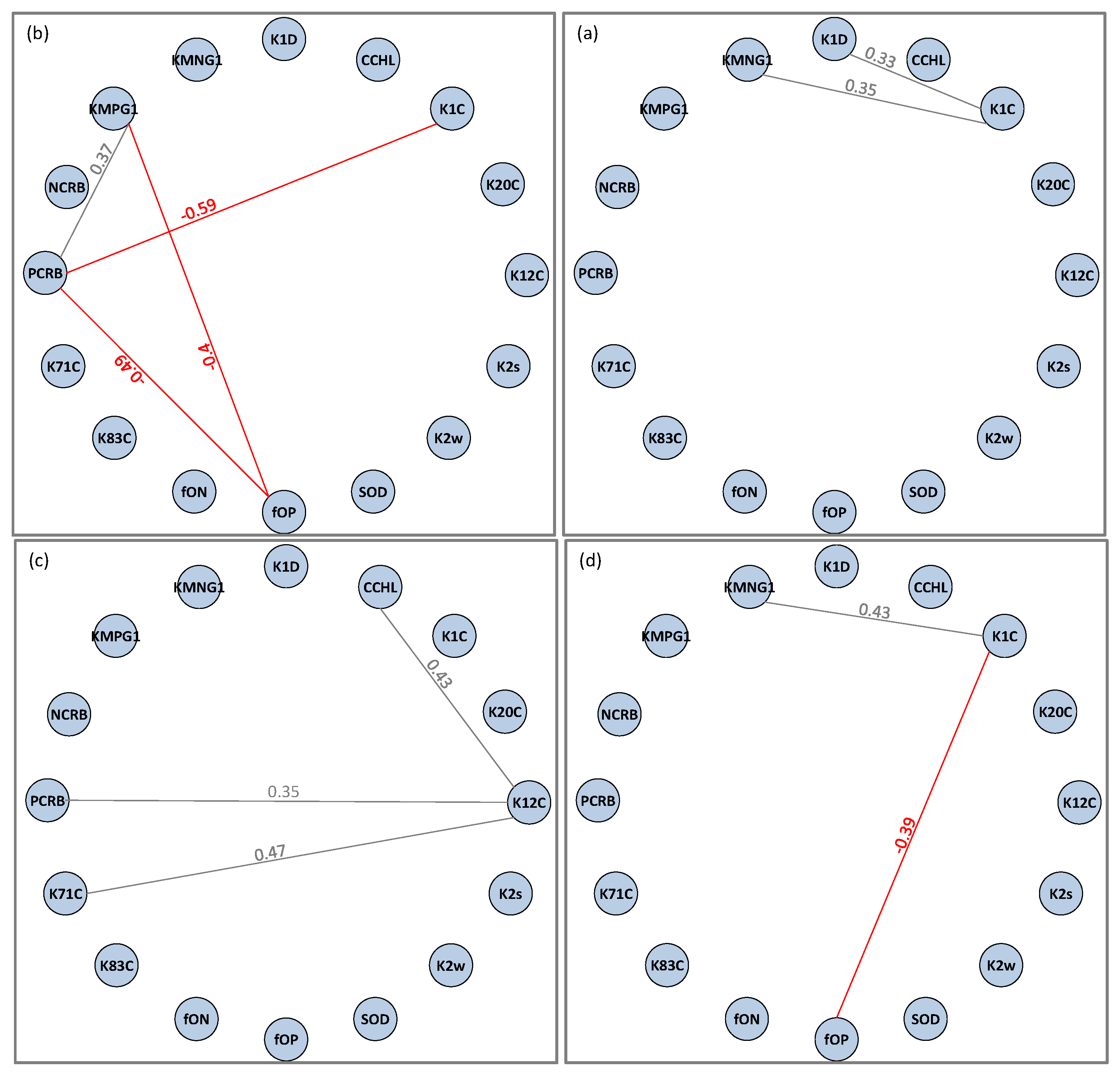
2.5. Variable Interactions

First, sensitive parameters and their ranges were identified based on the Monte Carlo simulations. To investigate the interactions between variables, Latin Hypercube sampling was used to create parameter sets, which could represent the parameter space in a small sample better than just a simple Monte Carlo [45].

In this study, we aimed to examine the potential relationship between state variable correlations and the integrity of an ecosystem. The method used in this study for measuring the structure of correlation maps was the hierarchy index (h) [46]:

$$h=\frac{12}{(N-1)(N(N+1)}{\displaystyle \sum }_i^{}{[\frac{od(v_i)-({{\displaystyle \sum }}^{\text{}}od(v_i))}{N}]}^2$$

(4)

$$od(v_i)={\displaystyle \sum }_{k=1}^N{\overline{a}}_{ki}$$

(5)

where N is the total number of variables and od_(vi) or outdegree is the sum of absolute values of correlations between a variable and the adjacent variables.

In order to test this hypothesis, we compared the hierarchy index and water quality index (WQI) values. The WQI values were calculated from measured data using CCME (Canadian Council of Ministers of the Environment) water quality index formulas.

3. Results and Discussion

3.1. Global Sensitivity Analysis (GSA)

The GSA results for stations along the SSR are presented in

Table 2. Sensitivity analysis in winter.

Winter	NH4				NO3				ON				OPO4				OP				CHLA				DO
Parameters/ Segments	a	b	c	d	a	b	c	d	a	b	c	D	a	b	c	d	a	b	c	d	a	b	c	d	a	b	c	d
K12C	●				●	●																			●
K20C
K1C	●	●	○	●			●	●	●	●			●	●	●	●					●	●		●	●
CCHL	○								●			●	●	○		○				●	○
K1D			●	○					○					●	●	●					●	●	●	●
KMNG1								●
KMPG1	●	●					●	○					●	●								●		○
NCRB	●	●	○				○	●
PCRB		●											●	●	●	●					○	●
K71C	●	●	●	●					●	●	●	●
K83C																●	●	●	●	●
fON		●	●	●
fOP														●	●	●
SOD																									●	●	●	●
K2w																○									●	○
K2s

●- very significant (α < 0.001); ○- medium significance (0.001 <α < 0.01); blank-low significance (α > 0.01); (a) uSSR at Medicine Hat; (b) uSSR at Leader; (c) lSSR at Outlook, and (d) lSSR at Clarkboro Ferry.

and

Table 3. Sensitivity analysis in summer.

Summer	NH4				NO3				ON				OPO4				OP				CHLA				DO
Parameters/ Segments	a	b	c	d	a	b	c	d	a	b	c	D	a	b	c	d	a	b	c	d	a	b	c	d	a	b	c	d
K12C	●	●	●	●	●	●	●	●																	●			●
K20C
K1C							●						●	●	●	●		●			●	●	●	●		●
CCHL				●														●						●
K1D							●			○				○	●	●		●			●	●	●	●
KMNG1
KMPG1														○	●	●						●	●
NCRB				○
PCRB		○											●		●	●		●			○	●				●
K71C	●		●	●	○				●	●	●	●
K83C																	●	●	●	●
fON							●
fOP				○										●	●	●					●
SOD		○																							●	●	●	●
K2w																												○
K2s																											●

●- very significant (α < 0.001); ○- medium significance (0.001<α < 0.01); blank-low significance (α > 0.01); (a) uSSR at Medicine Hat; (b) uSSR at Leader; (c) lSSR at Outlook, and (d) lSSR at Clarkboro Ferry

for winter and summer. The parameter sensitivity was classified using the significance level (α) of differences between the behavioral and a priori distributions. High significance was attributed to parameters with α < 0.001, medium significance was attributed to parameters with 0.001 < α < 0.01, and no significance was attributed to α > 0.01.

Although there were some differences in parametric sensitivities at different locations along the river, similar trends in the dominant controls were found at these locations. For example, phytoplankton growth (K1C) and death (K1D) rates, TON mineralization (K71C), and phosphorus-carbon (CCHL) ratio were found to be sensitive at all the locations. Denitrification rate (K20C), reaeration rate (K2), 1/2 saturation for N-limitation on phytoplankton uptake (KMNG1), and the fraction of phytoplankton death recycled to ON (fON) did not show a large impact on variables. A smaller number of parameters were sensitive to variables simulated at the Medicine Hat station (prior to the RDR confluence) in summer and at the Outlook station (downstream of Lake Diefenbaker) in winter.

NH4, ON, and OPO4 were more sensitive under ice-covered conditions than in open water. In contrast, CHLA and DO were more sensitive in summer. The transformation of ammonium to nitrate was pronounced in summer with nitrification rate (K12C) being the most influential parameter for the NH4 and NO3 variables. The temperature dependency of nitrification was consistent with the results of the study by Shammas [47]. NH4 and ON were sensitive to TON mineralization (K71C), both in summer and winter, which indicates that the bacterial decomposition of organic nitrogen to ammonium was not seasonally affected. Similarly, TOP mineralization rate (K83C) was the dominant control on OP in summer and winter. Other than phytoplankton related parameters, CHLA was found to be sensitive to the phosphorus-related parameters but not to the nitrogen-related parameters. CHLA and OPO4 showed sensitivities to various similar parameters, suggesting that a strong linage between these two variables may exist. For the DO variable, SOD shows a high sensitivity, suggesting a strong interaction between the water column and the sediments.

The results presented above were based on the Monte-Carlo analysis framework with 1000 model simulations. Additional simulations were not necessary since the model outcome was stabilized by this number of simulations runs. However, our preliminary analysis showed that 1000 simulations were sufficient to yield relatively robust results.

The uncertainty in water quality variable is described here using the coefficient of variation defined as the ratio of the standard deviation to the mean [48]. In Figure 3, a comparison is made between the water quality variables distributions at two locations (1) in uSSR at Leader and (2) lSSR at Clarkboro Ferry in winter and summer. The uncertainty in uSSR is larger than the uncertainty in lSSR. NH4 in summer and OPO4 and CHLA in both winter and summer have larger uncertainties compared to the other water quality variables.

We studied the nutrient and light limitation results to determine the degree of light or nutrient deficiency for phytoplankton growth. The results indicate that phosphorus was the limiting factor for phytoplankton growth, except in winter when light was most limiting (see Figure 4). There is no evidence of nitrogen deficiency, which is consistent with the findings of Donald, et al. [29], who showed that phytoplankton growth in Lake Diefenbaker is phosphorus limited, specifically when light was sufficient. As expected, Outlook was the most phosphorus limited site (80% of the time) due to the phosphorus retentive effect of Lake Diefenbaker. Clarkboro Ferry was the least phosphorus limited site (71% of the time).

The interactions between parameters were examined using correlation maps for the best performing parameter sets (top 10%) from the Monte Carlo parameters (as presented in Figure 5). There were relatively weak correlations between parameters at all locations along the river. Phytoplankton growth rate (K1C) was directly or indirectly related to phosphorus-related parameters (i.e., KMPG1, fOP, and PCRB) at three stations along the SSR, Medicine Hat, Leader, and Clarkboro Ferry, highlighting the sensitivity of phytoplankton to the carbon:phosphorus ratio. At Outlook, there were some interactions between nitrification (K12C) and phosphorus-carbon ratio (PCRB), TON mineralization rate (K71C), and carbon-chlorophyll ratio (CCHL), suggesting that nitrogen may be slightly more limiting at that site. The weak relationships between parameters may be a result of the large number of parameters used for our Monte-Carlo analysis (high degrees of freedom). Therefore, the parameter effects are easily compensated by other parameter settings leading to weaker interactions between parameters.

3.2. Interactions between State Variables

The most sensitive parameters were selected using the Kolmogorov–Smirnov test. The parameters were ranked in order of importance for each model (uSSR and lSSR models), as shown in

Table 4. Parameter ranking in order of significance and the optimal ranges.

Parameters	Rank		P-Values from KS Test		Optimal Range
	uSSR	lSSR	uSSR	lSSR	uSSR	lSSR
K12C	2	16	1.8×10–9	1	1–2	0–3
K20C	8	15	0.19	0.94
K1C	10	1	0.27	7.4 × 10–28	0.5–2.4	0–1.5
CCHL	6	9	0.05	0.58
K1D	4	3	2.4 × 10–6	1.4 × 10–10	0–0.12	0.1–0.25
KMNG1	15	11	0.95	0.61
KMPG1	7	5	0.13	2.7 × 10–4	0.005–0.018	0–0.05
NCRB	11	6	0.37	0.01
PCRB	5	4	4.0 × 10–4	5.0 × 10–6	0–0.08	0.125–0.24
K71C	3	8	1.6 × 10–6	0.33	0–0.18	0–1
K83C	12	13	0.57	0.71
fON	16	14	0.96	0.86
fOP	9	2	0.25	2.2 × 10–11	0.6	0–0.45
SOD	1	7	1.8 × 10–18	0.32	0–0.5	0–2.5
K2w	14	10	0.88	0.6
K2s	13	12	0.86	0.67

. Based on the results, the nitrification rate (K12C), phytoplankton growth rate (K1C), phytoplankton death rate (K1D), phosphorus-carbon ratio (PCRB), fraction of phytoplankton death recycled to OP (fOP), half-saturation for P-limitation on phytoplankton (KMPG1) and sediment oxygen demand (SOD) were the most sensitive parameters on the overall model output. The dot plots of the parameter values versus model performance (SNSE) were used to define the optimal parameter ranges. As an example, the red ovals in the dot plots for phytoplankton death rate (K1D) (as presented in Figure 6) point to the phytoplankton death rate (K1D) range with the lowest error between simulations and measured data.

The most sensitive parameters and their optimal ranges were used for Latin Hypercube sampling. To assess the potential interaction between the variables, 2187 (3^7, with 7 = number of parameters) parameter sets were selected. The simulation with the least sum of squared errors from the Monte Carlo simulations was used as the base simulation.

Figure 7 shows the correlation maps of water quality variables using a graph theory approach. Thicker lines between edges show stronger correlations between the variables. The gray and red lines are positive and negative correlations, respectively.

The correlation graphs at the lSSR at Outlook and Clarkboro Ferry illustrate two clusters; the first one includes DON, OP, OPO4, and CHLA, whereas the second includes inorganic nitrogen (NO3 and NH4). DO was weakly linked to inorganic nitrogen at Clarkboro Ferry. The results indicate that the biological production for lSSR was generally more phosphorus controlled, which is consistent with the limiting factor results in Figure 4.

At Medicine Hat, DON was disconnected from the other variables and two clusters (first cluster included OP, OPO4, CHLA and the second one included NO3+NH4) were both connected to DO. The relationships between variables were more complex at Leader. There were negative correlations between OPO4 and all other variables. The complexity of relationships may indicate the vulnerability of the uSSR water quality system downstream of the RDR inlet. A slight change in one of the water quality variables may affect all other variables.

The greater complexity in the correlation graph and poorer water quality (based on the observed data) at the Leader station motivated an examination of the relationship between the correlation between variables and water quality, by comparing the hierarchy index values (degree of connectivity) to the water quality indices at the four studied stations along the SSR. Figure 8 displays an inverse relationship between h values and WQIs.

The network representation of the correlation linkages between model state variable has been adapted and extended from ecological network theory, reviewed in Montoya et al. [49] and Inges et al. [50]. Those reviews highlight the description of network complexity in terms of the number of linkages between variables and the strength of those linkages. In our case, the magnitude of the correlations between the variable interactions in the model simulations represents the number and strength of these linkages. Montoya et al. [49] mention that more complexity may make a network more “fragile” in terms of resilience and persistence of ecosystem variables. This may be the case for the more complex network of the uSSR shown in Figure 8, which coincides with the more polluted state of the uSSR downstream of the Red Deer River confluence. Although there are more interactions (linkages) between the variables in the uSSR network compared to the lSSR network, the interactions are weaker (generally lower correlations) imposing less of a chance that the system exists at a stable equilibrium [49]. Moreover, weaker interactions tend to lead to more local equilibria that are less stable [50], which corroborates nicely with the greater equifinality of the model simulations.

4. Conclusions

This research studied parametric sensitivities to state variables of a water quality model for a large Prairie river, the SSR, in western Canada. A Monte-Carlo sensitivity analysis was carried out to study the global sensitivities of parameters on state variables at different locations along the SSR. The impact of nutrient loads from the RDR tributary had a great impact on the water quality of the SSR and a pronounced parametric sensitivity was observed downstream from this tributary inflow, compared to the other locations along the river.

We observed a seasonal trend in the sensitivity of parameters to the water quality variables. Chlorophyll-a and dissolved oxygen were more sensitive to parameters in summer than winter; however, unexpectedly, nitrogen and phosphorus showed higher sensitivities to a larger number of parameters in winter than in summer. This research highlights that phosphorus (mostly in summer) and light (mostly in winter) are the primary limiting factors for phytoplankton growth in the SSR.

This research is a novel study of the interactions among water quality parameters and variables as well as interactions between the state variables and ecosystem integrity. Phosphorus transforming processes have a strong correlation to chlorophyll-a, and inorganic nitrogen parameters are strongly correlated to each other. The correlation map is more complex for the Leader station, downstream of the RDR confluence, where significant interactions among all the variables were observed. Comparisons of hierarchy index values and water quality indices indicate that an increase in the degree of correlation among variables suggests a decline in the water quality of the system.

References

1. Hagy, J.D.; Boynton, W.R.; Keefe, C.W.; Wood, K.V. Chesapeake Bay, 1950–2001: Long-term change in relation to nutrient loading and river flow. Estuaries 2004, 27, 634–658. [Google Scholar] [CrossRef]
2. Smith, V.; Tilman, G.; Nekola, J. Eutrophication: impacts of excess nutrient inputs on freshwater, marine, and terrestrial ecosystems. Environ. Pollut. 1999, 100, 179–196. [Google Scholar] [CrossRef]
3. Ji, Z.-G. Hydrodynamics and Water Quality: Modeling Rivers, Lakes, and Estuaries; John Wiley & Sons: Hoboken, NJ, USA, 2008. [Google Scholar]
4. Prowse, T.D. River-ice ecology. I: Hydrologic, geomorphic, and water-quality aspects. J. Cold Region. Eng. 2001, 15, 1–16. [Google Scholar] [CrossRef]
5. Martin, N.; McEacherm, P.; Yu, T.; Zhu, D. Model development for prediction and mitigation of dissolved oxygen sags in the Athabasca River, Canada. Sci. Total Environ. 2012, 443, 403–412. [Google Scholar] [CrossRef] [PubMed]
6. Wagener, T.; Kollat, J. Numerical and visual evaluation of hydrological and environmental models using the Monte Carlo analysis toolbox. Environ Model. Softw. 2007, 22, 1021–1033. [Google Scholar] [CrossRef]
7. Razavi, S.; Gupta, H.V. What do we mean by sensitivity analysis? The need for comprehensive characterization of “Global” sensitivity in Earth and Environmental Systems Models. Water Resour. Res. 2015, 51, 3070–3092. [Google Scholar] [CrossRef]
8. Sun, X.Y.; Newham, L.; Croke, B.; Norton, J. Three complementary methods for sensitivity analysis of a water quality model. Environ Model. Softw. 2012, 37, 19–29. [Google Scholar] [CrossRef]
9. Nossent, J.; Elsen, P.; Bauwens, W. Sobol’sensitivity analysis of a complex environmental model. Environ. Model. Softw. 2011, 26, 1515–1525. [Google Scholar] [CrossRef]
10. Sudheer, K.P.; Lakshmi, G.; Chaubey, I. Application of a pseudo simulator to evaluate the sensitivity of parameters in complex watershed models. Environ Model. Softw. 2011, 26, 135–143. [Google Scholar] [CrossRef]
11. Reusser, D.E.; Zehe, E. Inferring model structural deficits by analyzing temporal dynamics of model performance and parameter sensitivity. Water Resour. Res. 2011, 47. [Google Scholar] [CrossRef]
12. Guse, B.; Reusser, D.E.; Fohrer, N. How to improve the representation of hydrological processes in SWAT for a lowland catchment—Temporal analysis of parameter sensitivity and model performance. Hydrol. Process 2014, 28, 2651–2670. [Google Scholar] [CrossRef]
13. Pfannerstill, M.; Guse, B.; Reusser, D.; Fohrer, N. Process verification of a hydrological model using a temporal parameter sensitivity analysis. Hydrol. Earth Syst. Sci. 2015, 19, 4365–4376. [Google Scholar] [CrossRef]
14. Lindenschmidt, K.-E.; Chun, K.P. Evaluating the impact of fluvial geomorphology on river ice cover formation based on a global sensitivity analysis of a river ice model. Can. J. Civil Eng. 2013, 40, 623–632. [Google Scholar] [CrossRef]
15. Brown, L.C.; Barnwell, T.O. The Enhanced Stream Water Quality Models QUAL2E and QUAL2E-UNCAS; Environmental protection Agency, Environmental Research Laboratory: Athens, GA, USA, 1987.
16. Chapra, S.C.; Pelletier, G.J. Qual2k: A Modeling Framework for Simulating River and Stream Water Quality: Documentation and Users Manual; Civil and Environmental Engineering Department, Tufts University: Medford, MA, USA, 2003. [Google Scholar]
17. Ambrose, R.; Wool, T.A.; Connolly, J.; Schanz, R.W. WASP4, A Hydrodynamic and Water-Quality Model-Model Theory, User’s Manual, and Programmer’s Guide; No. PB-88-185095/XAB; EPA-600/3-87/039; Environmental protection Agency, Environmental Research Laboratory: Athens, GA, USA, 1988.
18. Environmental Laboratory. CE-QUAL-RIV1: A Dynamic, One-Dimensional (Longitudinal) Water Quality Model for Streams: User’s Manual; Instruction Report EL-95-2; USACE Waterways Experiments Station: Vicksburg, MS, USA, 1995. [Google Scholar]
19. Francos, A.; Elorza, F.J.; Bouraoui, F.; Galbiati, L. Sensitivity analysis of distributed environmental simulation models: Understanding the model behaviour in hydrological studies at the catchment scale. Reliab. Eng. Syst. Saf. 2003, 79, 205–218. [Google Scholar] [CrossRef]
20. Van Griensven, A.; Francos, A.; Bauwens, W. Sensitivity analysis and auto-calibration of an integral dynamic model for river water quality. Water Sci. Technol. 2002, 45, 321–328. [Google Scholar]
21. Drolc, A.; Končan, J.Z. Water quality modelling of the river Sava, Slovenia. Water Res. 1996, 30, 2587–2592. [Google Scholar] [CrossRef]
22. Van Griensven, A.; Meixner, T.; Grunwald, S.; Bishop, T.; Diluio, M.; Srinivasan, R. A global sensitivity analysis tool for the parameters of multi-variable catchment models. J. Hydrol. 2006, 324, 10–23. [Google Scholar] [CrossRef]
23. Franceschini, S.; Tsai, C.W. Assessment of uncertainty sources in water quality modeling in the Niagara River. Adv. Water Resour. 2010, 33, 493–503. [Google Scholar] [CrossRef]
24. Kaufman, G.B. Application of the Water Quality Analysis Simulation Program (WASP) to Evaluate Dissolved Nitrogen Concentrations in the Altamaha River Estuary, Georgia. Master’s Thesis, University of Florida, Gainesville, FL, USA, 2003. [Google Scholar]
25. Lindenschmidt, K.-E. The effect of complexity on parameter sensitivity and model uncertainty in river water quality modelling. Ecol. Model. 2006, 190, 72–86. [Google Scholar] [CrossRef]
26. Abirhire, O.; North, R.L.; Hunter, K.; Vandergucht, D.M.; Sereda, J.; Hudson, J.J. Environmental factors influencing phytoplankton communities in Lake Diefenbaker, Saskatchewan, Canada. J. Gt. Lakes Res. 2015, 41, 118–128. [Google Scholar] [CrossRef]
27. North, R.L.; Johansson, J.; Vandergucht, D.M.; Doig, L.E.; Liber, K.; Lindenschmidt, K.-E.; Baulch, H.; Hudson, J.J. Evidence for internal phosphorus loading in a large prairie reservoir (Lake Diefenbaker, Saskatchewan). J. Gt. Lakes Res. 2015, 41, 91–99. [Google Scholar] [CrossRef]
28. Morales-Marín, L.; Wheater, H.; Lindenschmidt, K.-E. Assessing the transport of total phosphorus from a prairie river basin using SPARROW. Hydrol. Process. 2015, 29, 4144–4160. [Google Scholar] [CrossRef]
29. Donald, D.B.; Parker, B.R.; Davies, J.-M.; Leavitt, P.R. Nutrient sequestration in the Lake Winnipeg watershed. J. Gt. Lakes Res. 2015, 41, 630–642. [Google Scholar] [CrossRef]
30. Dubourg, P.; North, R.L.; Hunter, K.; Vandergucht, D.M.; Abirhire, O.; Silsbe, G.M.; Guildford, S.J.; Hudson, J.J. Light and nutrient co-limitation of phytoplankton communities in a large reservoir: Lake 1 Diefenbaker, Saskatchewan, Canada. J. Gt. Lakes Res. 2015, 41, 129–143. [Google Scholar] [CrossRef]
31. Hudson, J.; Vandergucht, D. Spatial and Temporal Patterns in Physical Properties and Dissolved Oxygen in Lake Diefenbaker, a Large Reservoir on the Canadian Prairies. J. Gt. Lakes Res. 2015, 41, 22–33. [Google Scholar] [CrossRef]
32. Di Toro, D.; Fitzpatrick, J.; Thomann, R. Water Quality Analysis Simulation Program (WASP) and Model Verification Program (MVP) Documentation; U.S. EPA-600/3-81-044; US Environmental Protection Agency (EPA): Duluth, MI, USA, 1983.
33. Connolly, J.P.; Winfield, R.P. A User’s Guide for WASTOX, A Framework for Modeling the Fate of Toxic Chemicals in Aquatic Environments. Part 1: Exposure Concentration; Environmental Research Laboratory, Office of Research and Development, US Environmental Protection Agency: Washington, DC, USA, 1984.
34. Akomeah, E.; Chun, K.P.; Lindenschmidt, K.-E. Dynamic water quality modelling and uncertainty analysis of phytoplankton and nutrient cycles for the upper South Saskatchewan River. Environ. Sci. Pollut. Res. 2015, 22, 18239–18251. [Google Scholar] [CrossRef] [PubMed]
35. Hosseini, C.W.L. Parameter sensitivity of a surface water quality model of the lower South Saskatchewan River—Comparison between ice-on and ice-off periods. ENMO 2016, submitted. [Google Scholar]
36. Saltelli, A.; Annoni, P. How to avoid a perfunctory sensitivity analysis. Environ. Model. Softw. 2010, 25, 1508–1517. [Google Scholar] [CrossRef]
37. Hornberger, G.M.; Spear, R.C. An approach to the preliminary analysis of environmental systems. J. Environ. Manag. 1981, 12, 7–18. [Google Scholar]
38. Sobol, I.M. Global sensitivity indices for nonlinear mathematical models and their Monte Carlo estimates. Math. Comput. Simul. 2001, 55, 271–280. [Google Scholar] [CrossRef]
39. Razavi, S.; Gupta, H.V. A new framework for comprehensive, robust, and efficient global sensitivity analysis: 1. Theory. Water Resour. Res. 2016, 52, 423–439. [Google Scholar] [CrossRef]
40. Razavi, S.; Gupta, H.V. A new framework for comprehensive, robust, and efficient global sensitivity analysis: 2. Application. Water Resour. Res. 2016, 52, 440–455. [Google Scholar] [CrossRef]
41. Matott, L.S. Ostrich: An Optimization Software Tool, Documentation and User’s Guide; Version 1.6; University at Buffalo, Department of Civil, Structural, and Environmental Engineering: Buffalo, NY, USA, 2005. [Google Scholar]
42. Wagener, T.; Wheater, H.S.; Gupta, H.V. Rainfall-Runoff Modelling in Gauged and Ungauged Catchments; Imperial College Press: London, UK, 2004. [Google Scholar]
43. Chapra, S.C. Surface Water Quality Modeling; McGraw-Hill Companies: New York, NY, USA, 1997. [Google Scholar]
44. Karrh, R. Nutrient Limitation. Available online: http://dnr.state.md.us/bay/monitoring/limit/index.html (accessed on 13 April 2016).
45. Saltelli, A.; Tarantola, S.; Campolongo, F.; Ratto, M. Sensitivity Analysis in Practice: A Guide to Assessing Scientific Models; John Wiley & Sons Inc.: Hoboken, NJ, USA, 2004. [Google Scholar]
46. MacDonald, N. Trees and Networks in Biological Models; John Wiley & Sons: New York, NY, USA, 1983. [Google Scholar]
47. Shammas, N.K. Interactions of Temperature, pH, and Biomass on the Nitrification Process. Water Pollut. Control Feder. 1986, 58, 52–59. [Google Scholar]
48. Lindenschmidt, K.-E.; Poser, K.; Rode, M. Impact of morphological parameters on water quality variables of a regulated lowland river. Water Sci.Technol. 2005, 52, 187–194. [Google Scholar] [PubMed]
49. Montoya, J.M.; Pimm, S.L.; Solé, R.V. Ecological networks and their fragility. Nature 2006, 442, 259–264. [Google Scholar] [CrossRef] [PubMed]
50. Ings, T.C.; Montoya, J.M.; Bascompte, J.; Blüthgen, N.; Brown, L.; Dormann, C.F.; Edwards, F.; Figueroa, D.; Jacob, U.; Jones, J.I.; et al. Review: Ecological networks—Beyond food webs. J. Anim.Ecol. 2009, 78, 253–269. [Google Scholar] [CrossRef] [PubMed]
Figure 1. Map of South Saskatchewan River Basin.
Water 08 00158 g001
Figure 2. Measured concentrations (A) dissolved oxygen; (B) total nitrogen; (C) chlorophyll-a, and (D) total phosphorus along the SSR, (a) uSSR at Medicine Hat; (b) uSSR at Leader; (c) lSSR at Outlook, and (d) lSSR at Clarkboro Ferry.
Water 08 00158 g002aWater 08 00158 g002b
Figure 3. Uncertainty in water quality variables. (a) winter; (b) summer.
Water 08 00158 g003
Figure 4. Nutrient and light limitations for the best performing simulation. (a) uSSR at Medicine Hat; (b) uSSR at Leader; (c) lSSR at Outlook, and (d) lSSR at Clarkboro Ferry.
Water 08 00158 g004
Figure 5. Parameter correlation: grey and red edges are positive and negative correlations, respectively. (a) uSSR at Medicine Hat, (b) uSSR at Leader, (c) lSSR at Outlook, and (d) lSSR at Clarkboro Ferry.
Water 08 00158 g005
Figure 6. Dot plots of parameter sets and objective functions for K1D. (a) uSSR; (b) lSSR.
Water 08 00158 g006
Figure 7. Correlation between variables. (a) uSSR at Medicine Hat; (b) uSSR at Leader; (c) lSSR at Outlook, and (d) lSSR at Clarkboro Ferry.
Water 08 00158 g007
Figure 8. Comparison of hierarchy indices and water quality indices.
Water 08 00158 g008