Article

Use of Bathymetric and LiDAR Data in Generating Digital Elevation Model over the Lower Athabasca River Watershed in Alberta, Canada

1
Department of Geomatics Engineering, Schulich School of Engineering, University of Calgary, 2500 University Drive NW, Calgary, AB T2N 1N4, Canada
2
Department of Civil Engineering, Schulich School of Engineering, University of Calgary, 2500 University Drive NW, Calgary, AB T2N 1N4, Canada
3
Alberta Environment and Parks, 2938 11 Street NE, Calgary, AB T2E 7L7, Canada
*
Author to whom correspondence should be addressed.
Water 2017, 9(1), 19; https://doi.org/10.3390/w9010019
Submission received: 9 November 2016 / Revised: 9 December 2016 / Accepted: 24 December 2016 / Published: 2 January 2017
(This article belongs to the Special Issue Geospatial Modeling of River Systems)

Abstract

:
The lower Athabasca River watershed is one of the most important regions for Alberta and elsewhere due to fact that it counts for the third largest oil reserve in the world. In order to support the oil and gas extraction, Athabasca River provides most of the required water supply. Thus, it is critical to understand the characteristics of the river and its watershed in order to develop sustainable water management strategies. Here, our main objective was to develop a digital elevation model (DEM) over the lower Athabasca River watershed including the main river channel of Athabasca River (i.e., approximately 128 km from Fort McMurray to Firebag River confluence). In this study, the primary data were obtained from the Alberta Environmental Monitoring, Evaluation and Reporting Agency. Those were: (i) Geoswath bathymetry at 5–10 m spatial resolution; (ii) point cloud LiDAR data; and (iii) river cross-section survey data. Here, we applied spatial interpolation methods like inverse distance weighting (IDW) and ordinary kriging (OK) to generate the bathymetric surface at 5 m × 5 m spatial resolution using the Geoswath bathymetry data points. We artificially created data gaps in 24 sections each in the range of 100 to 400 m along the river and further investigated the performance of the methods based on statistical analysis. We observed that the DEM generated using the both IDW and OK methods were quite similar, i.e., r2, relative error, and root mean square error were approximately 0.99, 0.002, and 0.104 m, respectively. We also evaluated the performance of both methods over individual sections of interest; and overall deviation was found to be within ±2.0 m while approximately 96.5% of the data fell within ±0.25 m. Finally, we combined the Geoswath-derived DEM and LiDAR-derived DEM in generating the final DEM over the lower Athabasca River watershed at 5 m × 5 m resolution.

1. Introduction

The lower Athabasca River watershed is one of the most important regions for Alberta and elsewhere due to fact that it counts for the third largest oil reserve in the world [1]. Thus, the region has been experiencing enormous expansion in extracting oil and gas since the 1960s. In fact, such activities require significant amount of water, where the Athabasca River is the most important source. Thus, it is critical to understand the characteristics of the river and its watershed in order to develop sustainable water utilization strategies, in particular to the face of climate change. In general, topography of a river bed (i.e., variation in the depths of a river commonly known as river bathymetry) is one of the major key components for the understanding of the characteristics of a river, and the topography of the surrounding flood-plains is another key component for the understanding of the entire watershed. Thus, we intend to develop a digital elevation model (DEM) for the entire lower Athabasca River watershed including the major river channel.
Traditionally, collecting river bathymetry data is a cumbersome process, which require data collection at several intervals along the river length. Typically, the river bathymetric information is comprised of sample data collected from a series of surveyed cross sections. In most cases, the sample data collection techniques were manual, time consuming, non-georeferenced, and locations of the cross-sections are based on the chainage (i.e., length of river sections from a reference known point) information of the river. Such techniques often lead to erroneous data, especially in the case of lateral movements of a river. Therefore, uncertainties were introduced during the generation of the bathymetric surfaces, while data interpolation techniques were applied over long distances in large rivers [2], e.g., the Athabasca River in Alberta. In the recent decades, modern surveying techniques have evolved to capture the fluvial geomorphologic characteristics to understand the river bathymetry and the flood plain topography [3,4,5]. Such development of geodetic survey techniques can provide further detail and higher spatial resolution bathymetry points (at centimeter level) in the form of point cloud data [6,7]. The data can be used to generate continuous topographical surfaces both for river (bathymetry surface) and flood-plains (topographical surface in the form of DEM).
Among the modern surveying techniques, photogrammetry, single and multi-beam sound navigation and ranging (SONAR), total station (TS), real time kinematic global positing system (RTK GPS), terrestrial laser scanning, airborne laser scanning, and remote-sensing based spectral signatures are intensively used in generating the topographic and bathymetric surfaces [8,9]. Most of these techniques are ground-based and airborne surveys. These techniques are capable of capturing precise elevations at sub-centimeter levels both in horizontal and vertical directions. These techniques generally captured the cross-section information in grid-based (i.e., X, Y, and Z) or topographically stratified datasets, which can be utilized in generating continuous surfaces by employing different interpolation techniques. Uncertainties of the interpolation techniques are subject to the quality of individual point observations, density of surveyed points, spatial resolution of the raster datasets, and strategy of survey (i.e., purpose, location, and timing [10]). Additionally, employing different interpolation techniques can produce different bathymetric or topographic surfaces even using the same input data [11]. These uncertainties are more prominent for dynamic rivers with steeper slopes and high topographic complexity, and most noticeable along the river banks, braided channels and islands [12]. In general, continuous surfaces of river bathymetry and flood plain topography are generated by employing several interpolation techniques based on survey data.
In recent times, the computational capabilities of river regime (i.e., geomorphological) have been augmented by using several modelling and interpolation methods. In the literature, we found various spatial interpolation techniques are available in generating the river bathymetric surfaces using numerous data sources, combined with the terrain dataset based on Light Detection and Ranging (LiDAR) and topographic surveys. These techniques can be classified into three categories, such as deterministic, geostatistical, and synergy between them to produce high resolution bathymetric surfaces and flood plain topography [13,14]. However, there is no consensus regarding the appropriate method that can be adopted for generating the best bathymetric and/or topographic surfaces. A few of the studies and methods used in generating the river bathymetric and flood-plain topographic surfaces are summarized below.
  • Schwendel et al. [8] investigated different interpolation methods for generating the digital elevation model (DEM) in four upland rivers in the Ruahine and Tararua Ranges over the southern part of New Zealand’s north island. The study used triangulation with linear interpolation, natural neighbours, point and universal kriging, multi-quadratic radial basis function, modified Shepard’s method, and inverse distance weighting (IDW) for four rivers reaches. The generated DEM using triangulation with linear interpolation ranked the best among all the methods used in the study (i.e., mean absolute error in the range of −0.01 to +0.003 m) while compared with the measured data.
  • The single-beam echo sounder and GPS-based river bathymetry data were used by Merwade [15] at six rivers reaches (i.e., Brazos, King Ranch, Rainwater, Sulphur located in Texas, and Kentucky and Ohio located in Kentucky) in the USA. Seven interpolation techniques were investigated (i.e., IDW, regularized spline, spline with tension, topo grid, natural neighbour, ordinary kriging (OK), and OK with anisotropy) using both with- and without-moving the trends. Four bathymetric surfaces were created using all seven methods (i.e., in total of 28 × 6 reaches). OK with anisotropy was found as the best, i.e., root mean square error (RMSE) values in the range of 0.2–1.0 m in all six reaches, compared with the validation datasets.
  • Kardos [16] used river cross sectional survey data (i.e., acoustic Doppler current profiler (ADCP)) to generate the bathymetric surfaces over the Paks-Mohács reach of Danube River in Hungary. The proposed method was comprised of the following steps: (a) cross-sectional data were orthogonally projected to a straight line keeping original z-value; (b) the straight line was divided into equal segments and z-value was computed using neighbourhood points; (c) an equidistance mesh was created between two cross-sections, and z-value was computed from surrounding four points; and (d) finally compared with the “topo to raster” and “natural neighbour” methods using full and partial datasets (i.e., considering every fifth cross-section data). The deviation between two surfaces (i.e., full and partial datasets) were found to be within ±1.0 m in case of low flow conditions, whereas it was found to have very limited usage in case of high-flow condition riverbeds.
  • Fonstad and Marcus [17] utilized local river gauge data (i.e., discharge), image brightness value (i.e., digital aerial photograph), and manning’s roughness to calculate the river bathymetric information (i.e., water depth) over the Brazos River, Texas and Lamar River, Wyoming. Two models were developed based on channel shape approximation and Beer-Lambert approximation. The average water depth was calculated as a function of discharge, river width, and slope values; and correlated with the image brightness [i.e., blue digital number (DN) values correlated well (r2 value of 0.76)]. The estimated water depth and measured depth were well correlated (i.e., r2 value 0.51 and 0.77, respectively, for the Brazos River; and r2 value 0.46 and 0.26, respectively, for the Lamar River).
  • The bathymetric information of Lake Vrana in Crotia was steered using an integrated measuring system, i.e., single beam SONAR data equipped with GPS, rover GPS, and dual frequency probe [18]. The coordinates and depth information were processed and further used to develop the continuous surfaces using 15 different interpolation methods (i.e., IDW, local polynomial, radial basis function, completely regularized spline, spline with tension, multi-quadric function, inverse multi-quadratic, OK, simple kriging, universal kriging, disjunctive kriging, ordinary cokriging, simple cokriging, universal cokriging, and disjunctive cokriging). Among them, the ordinary cokriging method was found as the best (i.e., standard deviation was less than 0.24 m).
  • Glenn et al. [19] investigated the effect of transect location, spacing, and interpolation methods in generating the river bathymetric surfaces in the Snake River and Bear Valley Creak in Idaho. High resolution aerial photographs and multi-beam SONAR survey data were used for the Snake River, and experimental advance airborne research LiDAR (EAARL) data were used for Bear Valley Creek. Four interpolation methods (i.e., Delaunay triangulation, simple linear and OK using curvilinear coordinates, and Delaunay triangulation and NN using Cartesian coordinates) were investigated using different sets of transect locations (i.e., morphologically and equally spaced). The authors found that the accuracy of the DEM was not a function of transect location or interpolation method, rather the coordinate system of the interpolation and spacing between transects.
  • Panhalkar and Jarag [20] used the surveyed cross-section data gathered by total station and differential GPS (DGPS) along a reach of 50 km over the Panchganga River in India. The IDW, Kriging and topo to raster methods were investigated to generate the river bathymetric surfaces. The authors observed that the IDW method performed better with a minimum standard RMS error of 0.776 m.
  • Conner and Tonina [21] investigated the effect of cross section-based interpolated bathymetry on 2D hydrodynamic-model results over the simple and complex reaches of the Snake River and the Hells Canyon in Idaho, USA. The authors used high resolution multi-beam SONAR data in conjunction with remotely sensed data. Several grid surfaces were generated based on complete data sets, and equally spaced cross-sections (i.e., 0.5, 1, 2, 3, 4 and 6 times of average channel width). The surfaces were generated using the IDW method in a curvilinear gridding system. They suggested that using cross section spacing in between 0.5 and 1.0 times of average width captured channel-geometry and other river flow properties are similar to complete bathymetry.
  • Hilldale and Raff [22] studied the river bathymetry in seven reaches of the Yakima and Naches Rivers (Yakima basin) in Washington, and one reach of the Trinity River in California, USA using airborne bathymetry LiDAR data. Universal kriging was used to generate the bathymetry surfaces and compared with the ground-based bathymetry data (i.e., collected using SONAR and bed elevations surveyed by wading). The authors used both point-based and grid-based comparison. The grid-based comparison showed a residual error (i.e., mean error) in the range of 0.15 to 0.29 m for the Yakima basin and 0.08 to 0.12 m for the Trinity River. The point-based comparison of the residuals also demonstrated similar results (i.e., 0.10 to 0.27 m and 0.12 to 0.18 m for the Yakima basin and Trinity River, respectively).
Thus, it is evident from the above review that various techniques have been used by researchers and practitioners for capturing bathymetric information, employing an interpolation algorithm, validating procedures, and utilizing them in river related research. It is recommended to use proper survey equipment for collecting bathymetry data depending on the characteristics of the river and the project. For large and complex rivers, elevation data should be collected in massive scale, e.g., point cloud data to generate grid. A complete grid of the river would provide the greatest level of detail and accuracy. It can be summarized that different interpolation techniques should be investigated, as generated surfaces from surveyed data may produce different map outputs using the same data.
In this study, we attempted to use available survey data from various sources, assess the quality of the source data, employ different interpolation techniques, and implement validation procedures in generating the continuous surface (i.e., DEM) of the river bathymetry of the lower Athabasca River watershed. The outcome of the DEM at 5 m × 5 m spatial resolution would help multiple levels in an organization’s hierarchy, such as planners, engineers, and decision makers in the delineation of catchment and sub-catchment boundaries, investigation of river morphology, calculation of environmental flow, analysis of hydrodynamic modelling, assessment of flood inundation and risk, allocation of surface water resources, etc. Thus, the overall objective of this research project is to develop a DEM for the selected reaches of the Athabasca River in the Province of Alberta. The specific objectives are to: (i) evaluate the quality of the available data; (ii) implement and evaluate the gap filling algorithms for both bathymetry and LiDAR data; and (iii) generate a DEM and its dynamics for the lower watershed area of the Athabasca River.

2. Materials

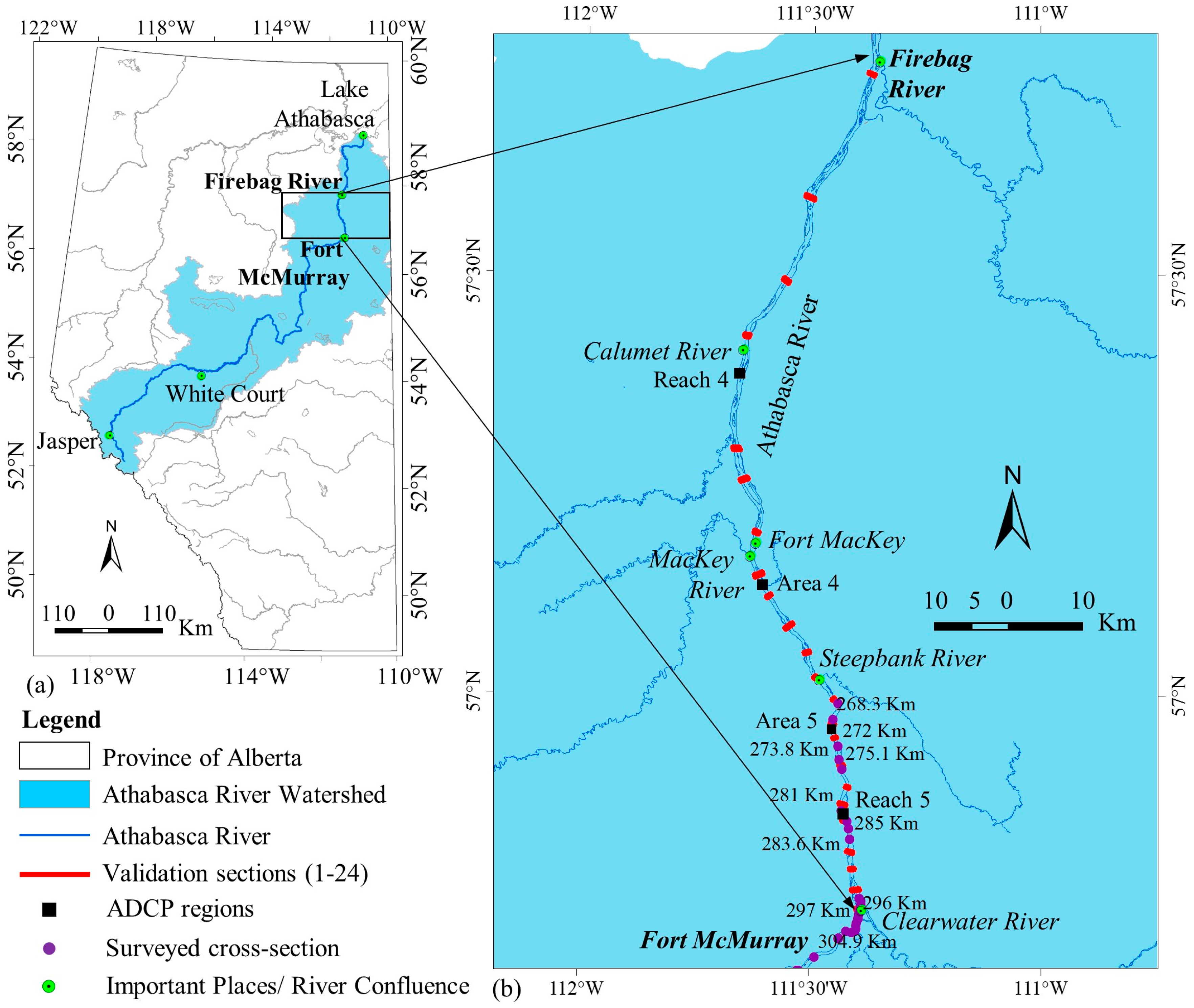
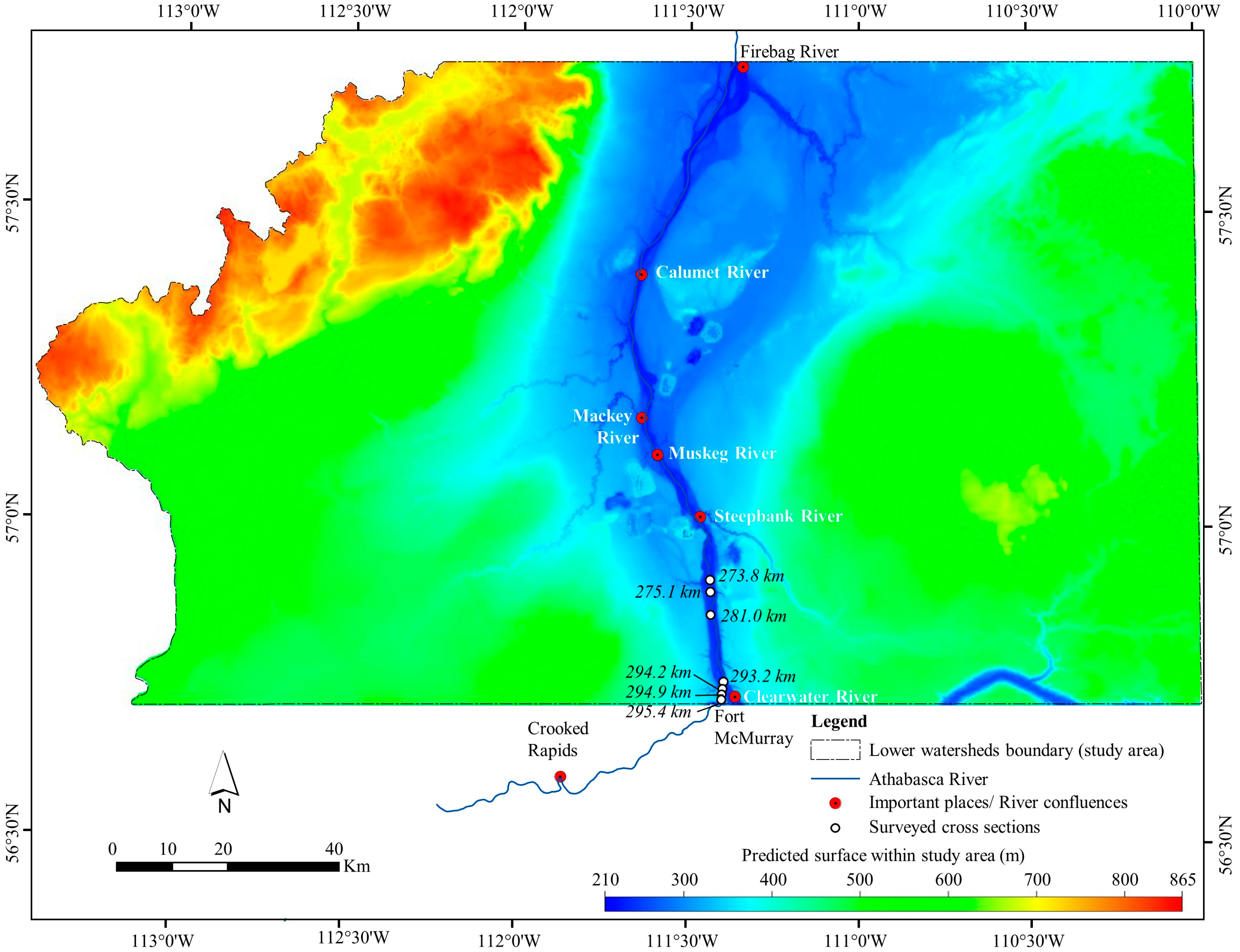
2.1. Description of the Study Area

The study area is located in the lower Athabasca River watershed, comprised of 128 km from Fort McMurray to the Firebag River confluence within the province of Alberta (Figure 1). The Athabasca River is approximately 1300 km in length, which is the second largest river in Alberta. The overall drainage area of the river is approximately 145,000 km2 before falling to the Lake Athabasca. The river consists of three reaches that are categorized as a function of topography and geological formation of the landscape [23]. Those are: (i) upper reach spans from the Columbia Ice Fields (the origin of the river) to the confluence of the McLeod River near the town of Whitecourt; (ii) middle reach stretches between the end of upper reach to the confluence of the Clearwater River near the city of Fort McMurray; and (iii) lower reach spans from the end of the middle reach to the Lake Athabasca. Note that several tributaries are contributing to the flows of the Athabasca River prior to concluding into the Lake Athabasca. The major tributaries include: (i) McLeod River, Prembina River, and Lesser Slave River in the middle reach; and (ii) Clearwater River, and Firebag River in the lower reach. The mean annual discharge varies along its extensive length and measured at different gauging stations within the above three reaches which are approximately 88.5, 430, and 660 m3/s, respectively [23].

2.2. Data Availability and Its Pre-Processing
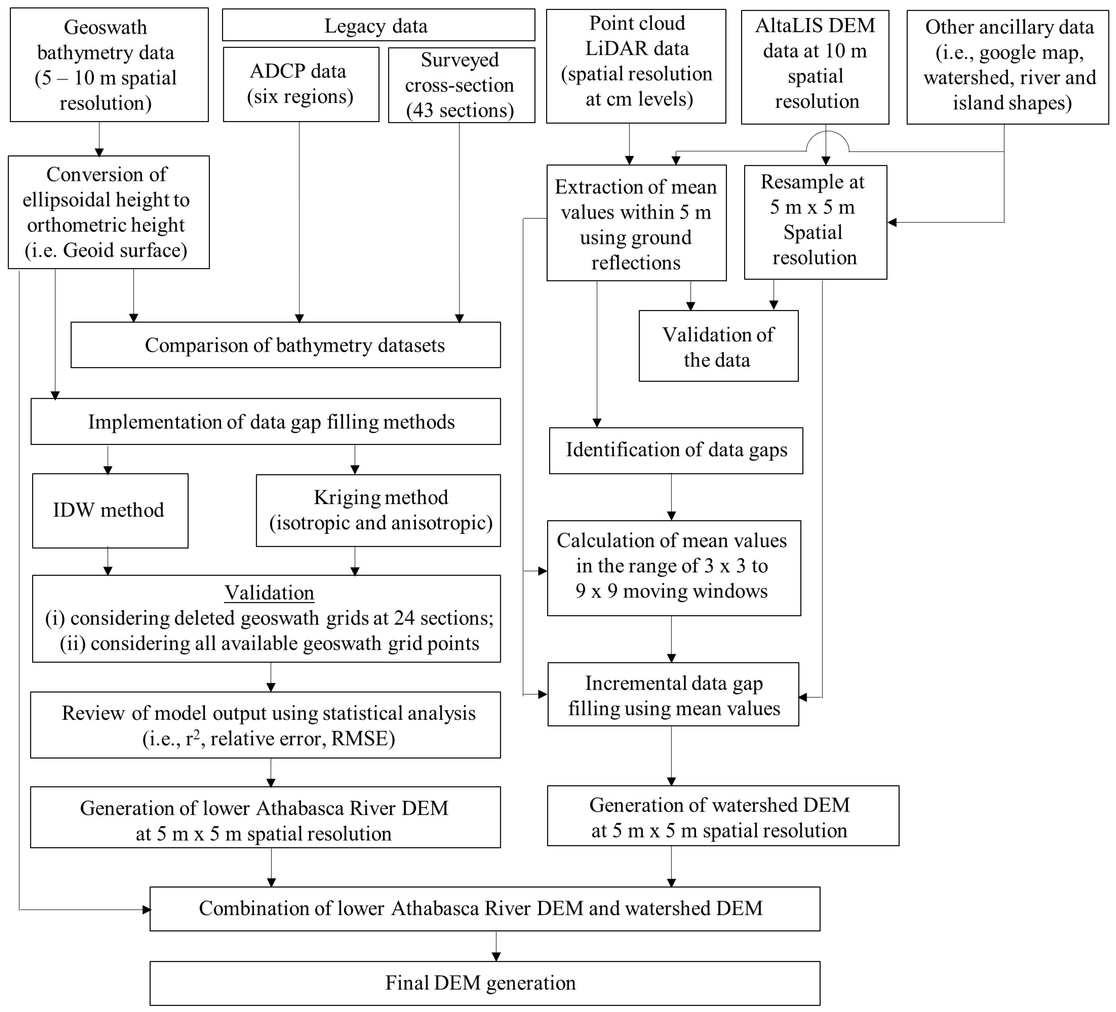
In our study, the primary data was obtained from the Alberta Environmental Monitoring, Evaluation and Reporting Agency (AEMERA). These included: (i) Geoswath bathymetry; (ii) point cloud LiDAR data; and (iii) legacy data (Table 1). In addition, we compiled other relevant ancillary data (i.e., administrative boundaries, major and minor rivers, the location of important places, watershed boundaries, and DEM at 10 m spatial resolution) available from the GIS data repository of University of Calgary and AltaLIS Ltd. (Digital Mapping of Alberta). The geographical features of the river and island were extracted at 1:20,000 scale under the Alberta Provincial Digital Mapping Program (accuracy within ±5 m). Most of these data were found in “geographical coordinate system” and subsequently converted into Universal Transverse Mercator (UTM, zone 12) projection system with North American Datum 83 (NAD83) version Canadian Spatial Reference System (CSRS). Furthermore, we extracted important locations and their identifiers from the Google map.
At first, the vertical measurements of Geoswath bathymetry data were converted from ellipsoidal height to orthometric height (i.e., Geoid surface). The height transformation desktop application package GPS.H 3.2.1 is a representation of Canadian Gravimetric Geoid Model 2013 and has been used in this study [25]. The point cloud LAS files were imported into ArcGIS environment to check the availability and extent of the dataset. Then, it was converted into multipoint data format in the ArcGIS environment considering the following conditions: (i) point spacing of the cloud data at 5 m; (ii) class code for the ground (i.e., 2); (iii) last return; (iv) intensity, return number, and number of return attributes; and (v) NAD83 (CSRS) UTM zone 12 projection system. Furthermore, multipoint LiDAR data were converted into a raster DEM at 5 m × 5 m spatial resolution. We observed that several areas were missing in the LiDAR data, which were subsequently filled using the other secondary data sources, such as 10 m DEM from AltaLIS (i.e., relative accuracy of ±5.0 m for X, Y, and Z). In addition, the delineation of the river cross-sections was done using the following steps: (i) information of the surveyed river cross-sections were converted into two separate datasets, i.e., cross-section location, and the bathymetric elevations; (ii) then, the cross-section location table was linked with the point shape file to extract the corresponding locations of the surveyed sections, and a point shape file was created for the 43 river cross-sections; and (iii) the generated cross-sectional data were linked with the attribute information of the cross-sections in ArcGIS. The ADCP data were checked for duplication and then converted to feature datasets in the geodatabase. Finally, all the available datasets were organized and integrated into a systematically designed geospatial database. Figure 2 shows the data processing procedures and methods employed during the study.

3. Methods

3.1. Data Quality

The river bathymetry dataset had issues like not covering the whole width of the river as well as gaps in the longitudinal direction (see Figure 3). Thus, we attempted to fill the data gaps by establishing a relationship between the Geoswath and ADCP regions, where the data points were common. We compiled all four ADCP regions, such as Reach 4 (Bitumount near Calumet River), Area 4 (Muskeg and the MacKey River), Area 5 (Steepbank River), and Reach 5 (Northlands). In this process, the Geoswath bathymetry raster data layer was superimposed with the ADCP data points and the corresponding elevation points were extracted. Then, we calculated r2 (coefficient of determination), slope, intercept, and RMSE values for the data quality assessment using the following equations. Furthermore, we extracted the Geoswath and ADCP bathymetry data corresponding to the generated cross-section locations and compared with respect to river widths and elevations. In addition, the data gaps in LiDAR were filled by implementing incremental gap filling algorithms in the range of 3 × 3, 5 × 5, 7 × 7, and 9 × 9, respectively. The additional gaps in the LiDAR data were subsequently filled from the AltaLIS digital elevation at 10 m spatial resolution (resampled at 5 m). We evaluated the extracted LiDAR data by comparing with the AltaLIS DEM and calculated the following statistical parameters (i.e., r2, slope, intercept, and RE values).
r 2 = [ i = 1 n ( O i O ¯ )   ( P i P ¯ ) i = 1 n ( O i O ¯ ) 2   i = 1 n ( P i P ¯ ) 2 ] 2
RMSE = 1 n i = 1 n ( O i P i ) 2

3.2. Gap Filling

In the literature, we observed that several spatial interpolation techniques were used to generate the bathymetry data based on survey samples depth, topographic data, and remote sensing based data, respectively [18,26,27,28,29]. Among those, sample depths collected at various reaches of the river have been widely used for river bathymetry generation and hydrodynamic studies [30,31]. Due to recent technological development, such methods of sample depth collection have the potential to capture more accurate river bathymetric information at higher resolution (i.e., approximately 1–5 m). We mentioned in earlier sections that the availability of the Geoswath bathymetry data in our study area were almost contiguous along the length of the Athabasca River from Firebag to Fort McMurray only within the water area. However, data gaps were visible in many places along the width of the river as shown in Figure 3. To fill the data gaps along the selected reaches of the Athabasca River, we used several interpolation techniques. The deterministic method, i.e., inverse distance weighting (IDW) and geostatistical method (i.e., ordinary kriging (OK) with both isotropy and anisotropy) were investigated to fill the data gaps within our area of interest. The ArcGIS Geostatistical Analyst tool has been used to implement such data gaps that were subsequently validated.
The IDW method describes the process of filling the missing data based on the philosophy on weighting among nearest neighbours (i.e., exact local interpolation technique) as represented by Watson and Philip [32], which estimates the values within the maximum and minimum of the sample-points. To calculate the value of an unknown point based on several known neighboured points can be described by the following equations:
P x = i = 1 n a i   P i
a i = ( 1 D i ) b i = 1 n ( 1 D i ) b   ,   i = 1 ,   2 ,   3     n
where j = 1 n a i = 1 , ai = weight factor for point location i, Px = value to be estimated at unknown point location, Pi = values at known point locations i, Di = distances from known points i to the point of estimation, b is the power to distance generally consider a value of 2, and n is the number of known point locations.
Kriging is a geostatistical method which has widely been used for spatial interpolation in generating river bathymetry [33]. This method assigns the weight (λ) based on surrounding known points by their distance, like IDW. In addition, it considers the spatial arrangement of the known points to estimate the value at unknown point location [34]. The spatial arrangement between the unknown and known points is based on the spatial autocorrelation and semivariogram (i.e., sill, range, lag and nugget values), which can be adjusted to model the spatial autocorrelation between the known points. The semivariogram and covariance functions may change both with distance and direction. Thus, in case of an anisometric model, both distance and direction variables are considered assuming that the sill may be reached earlier in other directions. However, in isometric model, it weights equally in all directions. Equation (5) shows the formula for interpolating the unknown point location based on known points.
P x = i = 1 n   λ i   P i   ,   i   =   1 ,   2 ,   3     n
where Px = value to be estimated at unknown point location, λi = unknown weight from known points i, Pi = values at known point locations i, and n is the number of known point locations.
In this study, we generated the bathymetric surface of the Athabasca River within the study area based on two conditions: (i) artificially deleting the Geoswath bathymetry data in 24 sections of the river in the range of 100 to 400 m in each section of interest; and (ii) considering all the available Geoswath bathymetry data. In both cases, we generated the predicted surface using IDW and Kriging methods. While performing the Kriging method, we changed the interpolation parameters interactively by altering the sill, range, lag and nugget values. The adjustment of the semivariogram was performed to model the autocorrelation of the existing Geoswath bathymetry data before performing the OK method (i.e., both isotropy and anisotropy cases). Then, we compared the generated surface with the existing Geoswath bathymetry data in the selected 24 sections. The validation was performed using a set of statistical measures, such as root mean squared error (RMSE) and coefficient of determination (r2) using the equations mentioned earlier in Section 3.1; and relative error (RE) and bias using the following mathematical expressions:
RE = ( O i P i ) 100 O i
Bias = 1 n   i = 1 n ( O i P i )
where n is the total number of observations, O i is the observed data, and P i is the predicted data.
The bathymetric surfaces generated by the interpolation methods were then investigated using the above statistical parameters, and the one with best performance was selected for the final DEM generation as discussed in the next sub-section.

3.3. DEM Generation

In generating the final DEM of the lower Athabasca River watershed, we combined the generated river DEM and other surveyed data as mentioned in earlier sections (e.g., LiDAR). Thus, the study reach of the Athabasca River DEM was comprised of three types of information, i.e., the river bathymetry, the island information within the river, and the floodplain. The main river bathymetry data were used from the generated surface (i.e., IDW), and subsequently replaced by the Geoswath data points where they were available. Thus, the bathymetry data over the area of interest were the combined effect of available Geoswath grid data points as well as data gaps filled from the generated predicted surface. The island elevations within the river were superimposed from the LiDAR data sets. In addition, floodplain data were also generated from the LiDAR data and finally combined with the Athabasca River DEM at 5 m × 5 m spatial resolution.

4. Results and Discussion

4.1. Data Quality

Table 2 shows the data quality assessment by means of r2, slope, intercept, RMSE, and RE values. The table shows that the relationship among the variables of interest (i.e., Geoswath and ADCP regions) were poor. The RMSE values were found in the range of 3.24, 1.69, 1.12 and 0.33 m for Area 4, Area 5, Reach 4, and Reach 5, respectively. However, other statistical parameters were poor for all four regions of interest. Thus, we might conclude from the analysis that the data gaps could not be filled from ADCP data set.
Furthermore, the Geoswath and ADCP data points were extracted corresponding to the surveyed cross sections measured from the left bank of the Athabasca River. We observed that a limited number of cross sections were matched with respect to the width and elevation. A wide range of values/differences were found in terms of both river widths and elevations for ADCP data compared with the surveyed cross section. This could be due to the difference in survey periods as those were conducted in different years, and the river-sections might be changed within this time frame. In case of ADCP data, most of the data extracted corresponding to the surveyed sections were found to be dubious. It was observed that the Geoswath data was relatively well represented in many sections with the surveyed cross section’s data except in a few cases. Thus, the Geoswath bathymetry data from Fort McMurray to the Firebag River confluence, approximately a length of 128 km (i.e., chainage from 294.58 km to 166.57 km) were used for generating the DEM. A total of 1,370,002 depth samples within the selected length were extracted from the Geoswath bathymetry data points. These bathymetry data included only the water area within the river during the survey periods, and many missing data points (i.e., small channels, dry river beds, islands, etc.) were visible along the river. It was evident that the bathymetric data within the area of interest observed an elevation range from 220 to 240 m with a mean value of 228 m and standard deviation of 4.85 m. Furthermore, we generated the slope of the lower Athabasca River by exploiting the bathymetry points at 500 m interval along the river center line. Figure 4 shows the longitudinal bed slope (i.e., average slope value of 0.000137) of the Athabasca River within the area of interest. Furthermore, we validated the LiDAR data with the AltaLIS DEM which revealed good results (i.e., r2, slope, intercept, and RE (%) values were 0.99, 1.00, −0.77, and 0.43, respectively).

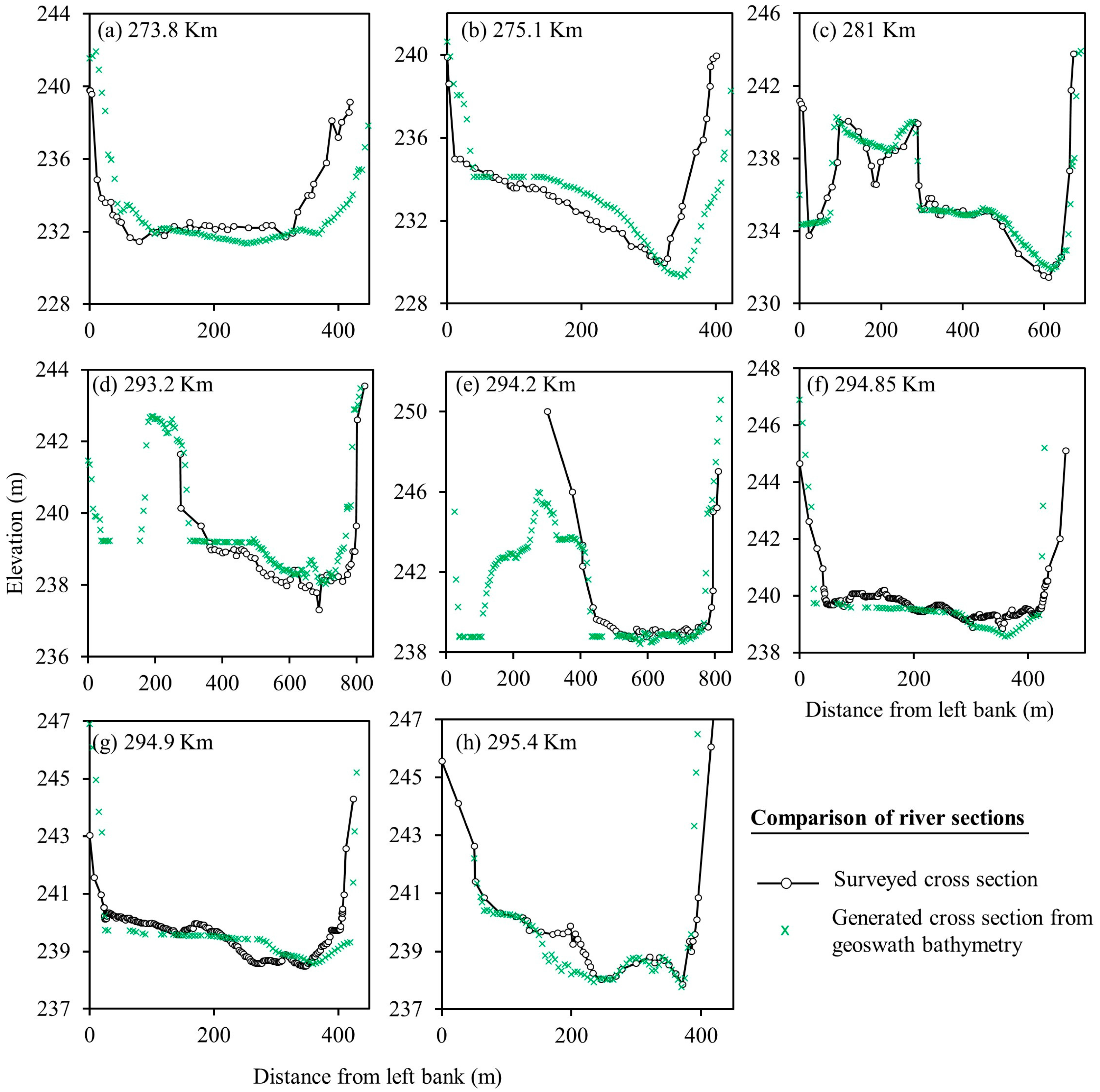
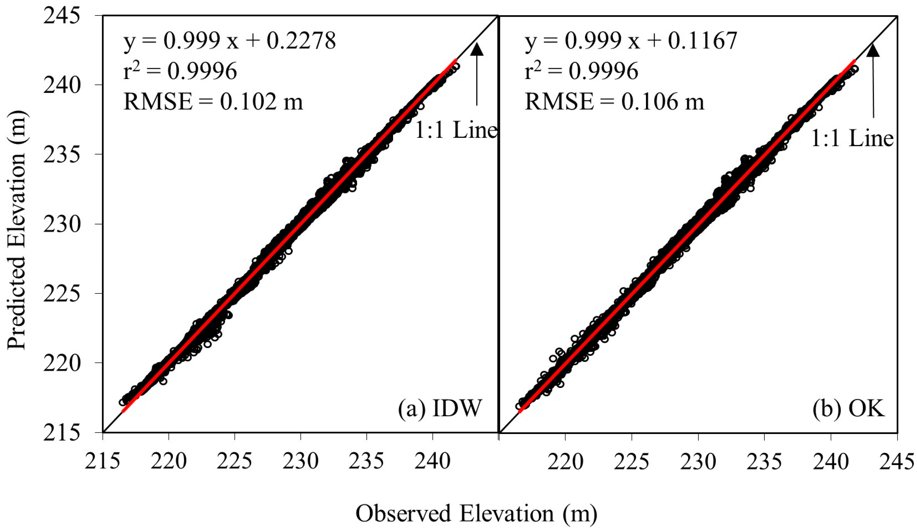
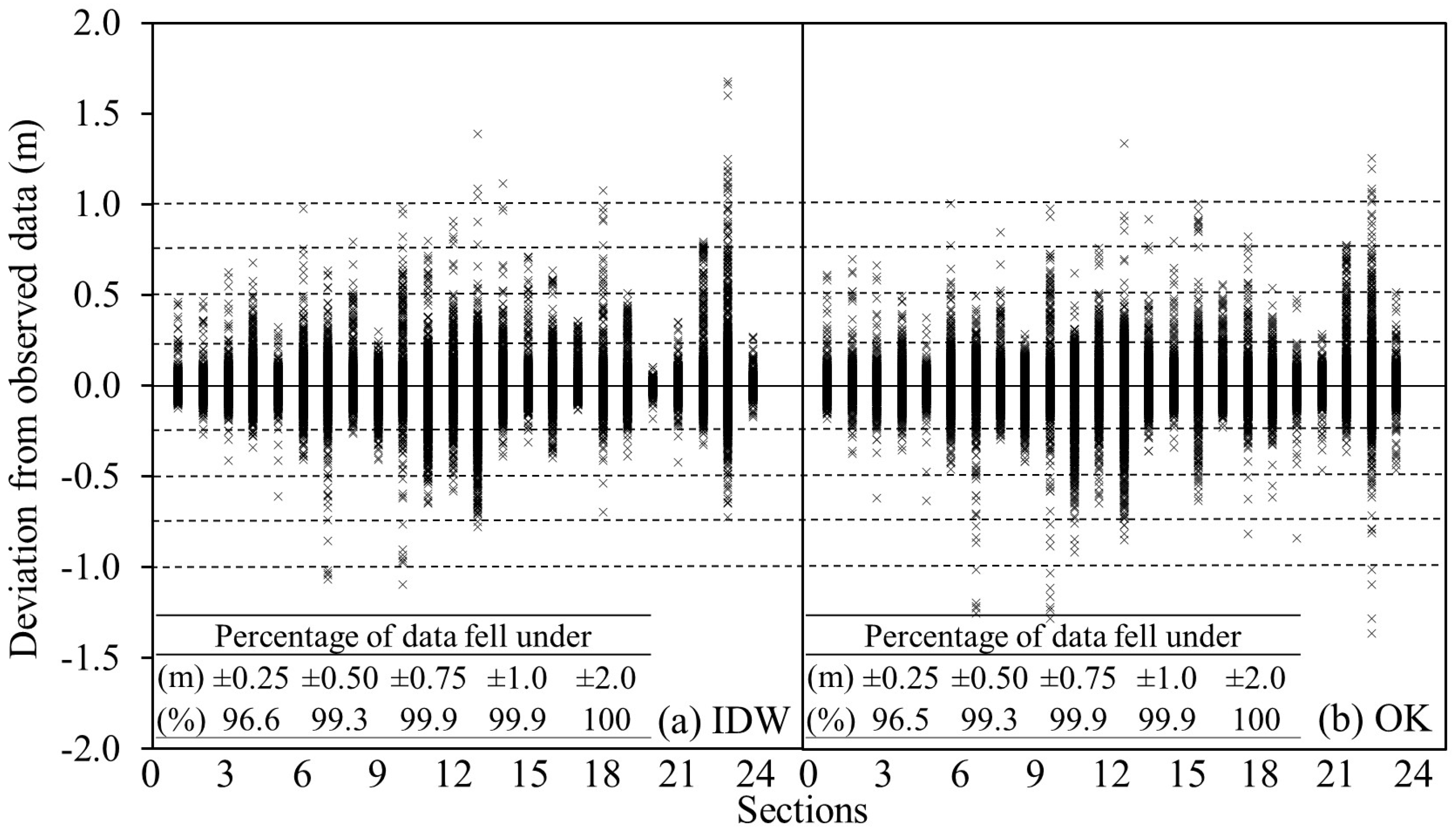
4.2. Comparison of Spatial Interpolation Methods

In this study, we attempted to investigate the performance of the different spatial interpolation methods for gap filling of the missing data and generated the DEM for the Athabasca River within the area of interest at 5 m × 5 m spatial resolution. In filling the data gaps, first we generated predicted surfaces using both IDW and OK (i.e., isotropic and anisotropic) methods after deleting grid points of 24 Geoswath sections (i.e., in the range of 100 m to 400 m for each section along the river length). The parameters of the IDW and OK methods were investigated to achieve the best results as shown in Table 3a. Then, we compared the predicted values of the 24 sections with the observed values, and calculated some statistical parameters as mentioned in earlier section. Table 4a shows the results of the methods which were investigated. We observed from Table 4a that the OK isotropic method performed better compared to the OK anisotropic method (i.e., RMSE value of 0.579 m in comparison to 0.668 m); and IDW method was found as the best (i.e., RMSE value of 0.478 m).
Finally, we generated surfaces using all the available Geoswath bathymetry data by employing the above methods (i.e., IDW and OK (isotropy)). The parameters of the spatial interpolation methods were shown in Table 3b. The relationship between the observed and predicted values is shown in Figure 5 upon exploiting grid points at 24 sections. We observed that the performances of the methods were similar in nature; however, the IDW method performed relatively better than the OK (isotropy) method as shown in Table 4b (i.e., Bias, r2, RMSE and RE (%) were found 0.003, 0.999, 0.102 and 0.001, respectively). It was observed that the methods applied to interpolate the depth samples yielded reliable results and might be helpful in river bathymetric related studies; such as in both 2-D and/or 3-D hydrodynamic modelling and research.
Furthermore, we calculated the deviation for each section of interest using both IDW and OK methods. Figure 6 shows the deviation of the predicted values at each individual point was in the range of ±2.0 m from the observed value. In addition, we grouped the above deviations into five elevation classes (i.e., 0.25, 0.50, 0.75, 1.00 and 2.00 m) considering all the 24 sections of interest (see Figure 6 for details). We found that about 96.5% of the grid data points fell within ±0.25 m. Only a nominal percentage of the grid data points (i.e., 0.05%) fell within ±1.0 m to ±2.0 m range. In fact, both the IDW and OK methods performed quite similarly, thus one of the methods could be adopted in this study. Our result was also similar in comparison to other studies found in the literature: (i) Curtarelli et al. [35] observed RMSE value of 0.92 m using OK (isotropy) geostatistical method to map the bathymetry of an Amazonian hydroelectric reservoir over Brazil; (ii) Panhalkar and Jarag [20] found the IDW method performed better (i.e., RMSE value of 7.63 m) in generating the bathymetry of Panchganga River over India; (iii) Merwade [15] observed that the OK anisotropic method achieved RMSE values in the range of 0.20 m to 0.80 m in six river reaches in the United States; and (iv) Moskalik et al. [36] investigated the bathymetry and geographical regionalization using OK method and found good relationship with the observed data (i.e., r2 value of 0.98) over Hornsund, Norway.

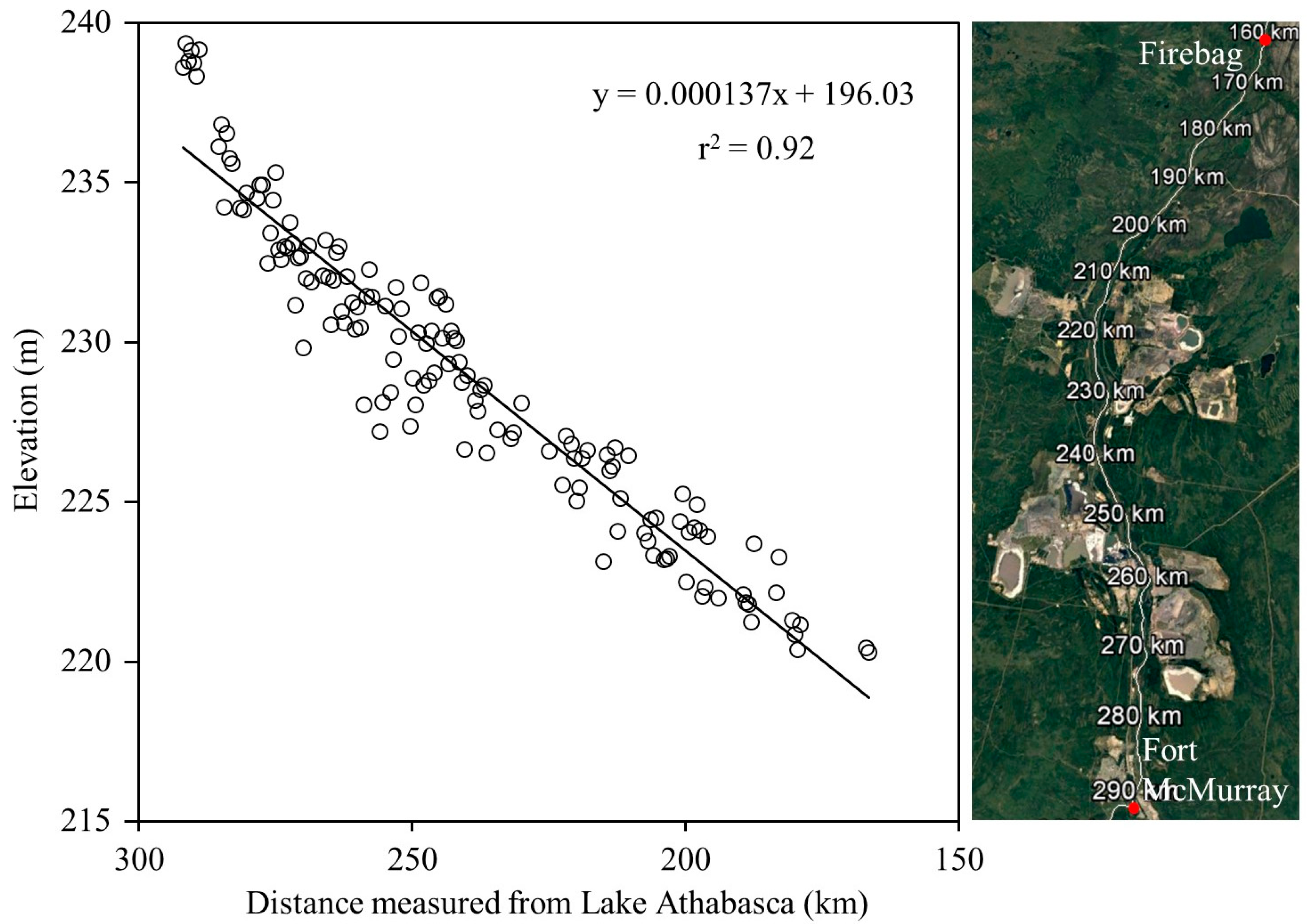
4.3. Final DEM Generation

Figure 7 shows the DEM of the lower Athabasca River watershed. Note that the water bodies within the flood plain (i.e., data processed from LiDAR) were not included in the final DEM, which was beyond the scope of the current study. After generating the final DEM, we extracted the cross-sectional information at several locations and compared those to the legacy river cross-section surveyed data. Figure 8 shows that the missing data across the river sections were filled, and matched with most of the surveyed sections.
However, some anomalies were observed with the surveyed cross sections that might be due to the following reasons: (i) time gaps of surveyed periods (i.e., comparison of the surveyed sections during 1977 to 2002 with Geoswath grid points during 2012 to 2014); (ii) river cross section surveyed data were available only for the main channels; (iii) planform changes or migration of the river laterally [37]; (iv) scouring and sedimentation along the river beds and islands are considered a dominant channel process [37,38]; (v) sediment regime was governed due to natural oil-sand deposits and releases of water, soil, and sediment from oil exploration in the study area [39,40]; and (vi) inaccuracies in the interpolated surface had influences from the neighbourhood grid data points [41], as different interpolation methods might produce different outputs using the same datasets [11].

5. Conclusions

In this article, we implemented simple protocols in generating DEM for the lower Athabasca River watershed at 5 m spatial resolution using Geoswath-derived bathymetric data for the major river channel (i.e., Athabasca River) and LiDAR-derived height data for the floodplain. Between the two spatial interpolation techniques of IDW and OK, we found that both produced similar results when compared against 24 selected sections (i.e., r2, RE and RMSE values were approximately 0.99, 0.002 and 0.104 m, respectively). Here, we studied only a part of the Athabasca River, i.e., approximately 128 km river reach. Thus, we strongly recommend production of the whole watershed DEM that will provide a platform for the planners and engineering practitioners for various river-based modelling exercises for better understanding and management of the hydro-morphological conditions. In addition, we would also like to note that the proposed framework should be thoroughly evaluated before implementing over other watersheds.

Acknowledgments

We would like to thank: (i) Alberta Environmental Monitoring, Evaluation and Reporting Agency (AEMERA) for providing a grant to Quazi K. Hassan and Gopal Achari; and (ii) National Sciences and Engineering Research Council of Canada for providing a Discovery Grant to Quazi K. Hassan. We appreciate all the data providing agencies, including: (i) Environment Canada; (ii) University of Alberta (Faye Hicks); (iii) Canadian Council of Ministers of the Environment; (iv) University of Calgary; and (v) AltaLIS Ltd. We also thankful to Natural Resource Canada for providing the height transformation desktop application package GPS.H 3.2.1. We also acknowledge the academic editor and anonymous reviewers for their valuable comments and suggestions in improving the overall quality of the manuscript.

Author Contributions

Conception and design: Ehsan H. Chowdhury, Quazi K. Hassan and Gopal Achari; data analysis, geodatabase preparation, and DEM generation: Ehsan H. Chowdhury; data provision: Anil Gupta; and manuscript preparation: Ehsan H. Chowdhury, Quazi K. Hassan, Gopal Achari and Anil Gupta.

Conflicts of Interest

The authors declare no conflict of interest.

References

  1. Natural Resources Canada (NRCAN). Oil Resources. Available online: http://www.nrcan.gc.ca/energy/oil-sands/18085 (accessed on 15 October 2016).
  2. Brasington, J.; Rumsby, B.; McVey, R. Monitoring and modelling morphological change in a braided gravel-bed river using high resolution GPS-based survey. Earth Surf. Proc. Landf. 2000, 25, 973–990. [Google Scholar] [CrossRef]
  3. Large, A.R.G.; Heritage, G.L. Laser scanning—Evolution of the discipline. In Laser Scanning for the Environmental Sciences; Heritage, G., Large, A.R.G., Eds.; Wiley Blackwell: West Sussex, UK, 2009; pp. 1–20. [Google Scholar]
  4. Milan, D.; Heritage, G.; Large, A.; Fuller, I. Filtering spatial error from DEMs: Implications for morphological change estimation. Geomorphology 2011, 125, 160–171. [Google Scholar] [CrossRef]
  5. Lyu, H.-M.; Wang, G.-F.; Shen, J.S.; Lu, L.-H.; Wang, G.-Q. Analysis and GIS mapping of flooding hazards on 10 May 2016, Guanzhou, China. Water 2016, 8, 447. [Google Scholar] [CrossRef]
  6. Rydlund, P.H., Jr.; Densmore, B.K. Methods of Practice and Guidelines for Using Survey-Grade Global Navigation Satellite Systems (GNSS) to Establish Vertical Datum in the United States Geological Survey; U.S. Geological Survey Techniques and Methods, Book 11, Chapter D1; U.S. Geological Survey: Reston, VA, USA, 2012; p. 102. Available online: http://pubs.usgs.gov/tm/11d1/ (accessed on 15 September 2016).
  7. Webster, T.; McGuigan, K.; Collins, K.; MacDonald, C. Integrated river and coastal hydrodynamic flood risk mapping of the LaHave River Estuary and town of Bridgewater, Nova Scotia, Canada. Water 2014, 6, 517–546. [Google Scholar] [CrossRef]
  8. Schwendel, A.C.; Fuller, I.C.; Death, R.G. Assessing DEM interpolation methods for effective representation of upland stream morphology for rapid appraisal of bed stability. River Res. Appl. 2012, 28, 567–584. [Google Scholar] [CrossRef]
  9. Allouis, T.; Bailly, J.; Pastol, Y.; Le Roux, C. Comparison of LiDAR waveform processing methods for very shallow water bathymetry using Raman, near-infrared and green signals. Earth Surf. Proc. Landf. 2010, 35, 640–650. [Google Scholar] [CrossRef]
  10. Heritage, G.L.; Milan, D.J.; Large, A.R.G.; Fuller, I.C. Influence of survey strategy and interpolation model on DEM quality. Geomorphology 2009, 112, 334–344. [Google Scholar] [CrossRef]
  11. Chilès, J.-P.; Delfiner, P. Geostatistics: Modeling Spatial Uncertainty, 2nd ed.; John Wiley & Sons Inc.: Hoboken, NJ, USA, 2012; p. 734. [Google Scholar]
  12. Charlton, M.E.; Large, A.R.G.; Fuller, I.C. Application of airborne LiDAR in river environments: The River Coquet, Northumberland, UK. Earth Surf. Proc. Landf. 2003, 28, 299–306. [Google Scholar] [CrossRef]
  13. Li, J.; Heap, A.D. Spatial interpolation methods applied in the environmental sciences: A review. Environ. Model. Softw. 2014, 53, 173–189. [Google Scholar] [CrossRef]
  14. Cho, H.; Hong, S.; Kim, S.; Park, H.; Park, I.; Sohn, H.-G. Application of a Terrestrial LIDAR System for Elevation Mapping in Terra Nova Bay, Antarctica. Sensors 2015, 15, 23514–23535. [Google Scholar] [CrossRef] [PubMed]
  15. Merwade, V. Effect of spatial trends on interpolation of river bathymetry. J. Hydrol. 2009, 371, 169–181. [Google Scholar] [CrossRef]
  16. Kardos, M. Interpolating river’s morphological model from cross sectional survey. In Second Conference of Junior Researchers in Civil Engineering; Budapest University of Technology and Economics (BME): Budapest, Hungary, 2013; pp. 243–248. Available online: https://www.me.bme.hu/doktisk/konf2013/papers/243-248.pdf (accessed on 15 February 2016).
  17. Fonstad, M.A.; Marcus, W.A. Remote sensing of stream depths with hydraulically assisted bathymetry (HAB) models. Geomorphology 2005, 72, 320–339. [Google Scholar] [CrossRef]
  18. Šiljeg, A.; Lozíc, S.; Šiljeg, S. A comparison of interpolation methods on the basis of data obtained from a bathymetric survey of Lake Vrana, Croatia. Hydrol. Earth Syst. Sci. 2015, 19, 3653–3666. [Google Scholar] [CrossRef]
  19. Glenn, J.; Tonina, D.; Morehead, M.D.; Fiedler, F.; Benjankar, R. Effect of transect location, transect spacing and interpolation methods on river bathymetry accuracy. Earth Surf. Proc. Landf. 2016, 41, 1185–1198. [Google Scholar] [CrossRef]
  20. Panhalkar, S.S.; Jarag, A.P. Assessment of spatial interpolation techniques for river bathymetry generation of Panchganga River basin using geoinformatic techniques. Asian J. Geoinform. 2015, 15, 9–15. [Google Scholar]
  21. Conner, J.T.; Tonina, D. Effect of cross-section interpolated bathymetry on 2D hydrodynamic model results in a large river. Earth Surf. Proc. Landf. 2013, 39, 463–475. [Google Scholar]
  22. Hilldale, R.C.; Raff, D. Assessing the ability of airborne LiDAR to map river bathymetry. Earth Surf. Proc. Landf. 2008, 33, 773–783. [Google Scholar] [CrossRef]
  23. Regional Aquatics Monitoring Program (RAMP). Athabasca River Basin. Available online: http://www.ramp-alberta.org/river.aspx (accessed on 20 November 2015).
  24. Canadian Council of Ministers of the Environment (CEMA). Lower Athabasca Data. Available online: http://ftp.cciw.ca/incoming/LowerAthabasca_data_March05.12/ (accessed on 5 December 2015).
  25. Natural Resources Canada (NRCAN). Height Reference System Modernization. Available online: http://www.nrcan.gc.ca/earth-sciences/geomatics/geodetic-reference-systems/9054 (accessed on 10 January 2016).
  26. El-Hattab, A.I. Single beam bathymetry data modelling techniques for accurate maintenance dredging. Egypt. J. Remote Sens. Space Sci. 2014, 17, 189–195. [Google Scholar]
  27. Hell, B.; Jakobsson, M. Gridding heterogeneous bathymetric data sets with stacked continuous curvature splines in tension. Mar. Geophys. Res. 2011, 32, 493–501. [Google Scholar] [CrossRef]
  28. Gao, J. Bathymetric mapping by means of remote sensing: Methods, accuracy and limitations. Prog. Phys. Geogr. 2009, 33, 103–116. [Google Scholar] [CrossRef]
  29. Jawak, S.D.; Vadlamani, S.S.; Luis, A.J. A synoptic review on deriving bathymetry information using remote sensing technologies: Models, Methods and Comparisons. Adv. Remote Sens. 2015, 4, 147–162. [Google Scholar] [CrossRef]
  30. Ler, L.G.; Holz, K.-P.; Choi, G.W.; Byeon, S.J. Tidal Data Generation for Sparse Data Regions in Han River Estuary Located in the Trans-Boundary of North and South Korea. Int. J. Control Autom. 2015, 8, 203–214. [Google Scholar] [CrossRef]
  31. Uddin, M.; Alam, J.B.; Khan, Z.H.; Hasan, G.M.J.; Rahman, T. Two dimensional hydrodynamic modelling of Northern Bay of Bengal coastal waters. Comput. Water Energy Environ. Eng. 2014, 3, 140–151. [Google Scholar] [CrossRef]
  32. Watson, D.F.; Philip, G.M. A refinement of inverse distance weighted interpolation. Geo-Processing 1985, 2, 315–327. [Google Scholar]
  33. Oliver, M.A.; Webster, R. Kriging: A method of interpolation for geographical information systems. Int. J. Geogr. Inf. Syst. 1990, 4, 313–332. [Google Scholar] [CrossRef]
  34. Longley, P.A.; Goodchild, M.F.; Maguire, D.J.; Rhind, D.W. Geographic Information Systems and Science, 3rd ed.; John Wiley & Sons, Ltd.: Hoboken, NJ, USA, 2010; p. 560. [Google Scholar]
  35. Curtarelli, M.; Leão, J.; Ogashawara, I.; Lorenzzetti, J.; Stech, J. Assessment of spatial interpolation methods to map the bathymetry of an Amazonian hydroelectric reservoir to aid in decision making for water management. ISPRS Int. J. Geo-Inf. 2015, 4, 220–235. [Google Scholar] [CrossRef]
  36. Moskalik, M.; Grabowiecki, P.; Tegowski, J.; Żulichowska, M. Bathymetry and geographical regionalization of Brepollen (Hornsund, Spitsbergen) based on bathymetric profiles interpolations. Pol. Polar Res. 2013, 34, 1–22. [Google Scholar] [CrossRef]
  37. Neill, C.R. Hydraulic and Morphologic Characteristics of Athabasca River near fort Assiniboine—The Anatomy of a Wandering Gravel River; Report REH/73/3; Alberta Cooperative Research Program, Highway and Engineering Division: Edmonton, AB, Canada, 1973; p. 23. [Google Scholar]
  38. Hooke, J.M. River channel adjustment to meander cutoffs on the River Bollin and River Dane, Northwest England. Geomorphology 1995, 14, 235–253. [Google Scholar] [CrossRef]
  39. Carson, M.A. Sediment Budget for the Athabasca River Basin, Alberta, between Fort McMurray and Embarras, 1876–1986; Report for the Inland Waters Directorate; Environment Canada: Calgary, AB, Canada, 1990; p. 42.
  40. Hebben, T. Analysis of Water Quality Conditions and Trends for the Long-Term River Network: Athabasca River, 1960–2007; Alberta Environment, Water Policy Branch, Environmental Assurance: Edmonton, AB, Canada, 2009; p. 341. Avaiable online: http://aep.alberta.ca/water/programs-and-services/surface-water-quality-program/documents/WaterQualityTrendsAthabascaRiver-Mar2009.pdf (accessed on 15 September 2016).
  41. Merwade, V.M.; Maidment, D.R.; Goff, J.A. Anisotropic considerations while interpolating river channel bathymetry. J. Hydrol. 2006, 331, 731–741. [Google Scholar] [CrossRef]
Figure 1. (a) Location of the Athabasca River watershed within the Province of Alberta; and (b) extent of the study area within the watershed.
Water 09 00019 g001
Figure 2. The conceptual diagram of gap filling methods and generation of lower Athabasca River watershed DEM.
Water 09 00019 g002
Figure 3. Geoswath bathymetry data gaps at selected locations.
Water 09 00019 g003
Figure 4. The longitudinal bed profile of the Athabasca River from Fort McMurray to the Firebag River confluence (elevation data were extracted along the center line of the river at 500 m interval).
Water 09 00019 g004
Figure 5. Comparison of the observed and predicted elevation values using both (a) IDW and (b) OK methods in selected 24 sections.
Water 09 00019 g005
Figure 6. Deviation of the predicted values from the observed data for both (a) IDW and (b) OK methods in selected 24 sections.
Water 09 00019 g006
Figure 7. The lower Athabasca River watershed DEM at 5 m × 5 m spatial resolution.
Water 09 00019 g007
Figure 8. Comparison of the predicted surface with surveyed cross sections.
Water 09 00019 g008
Table 1. Brief description of the primary data used in the current study.
Data TypeDescriptionSource
Geoswath bathymetryThis data has a horizontal spatial resolution of 5–10 m from Fort McMurray to Firebag river confluence (2012–2014).Environment Canada
Point cloud LiDAR dataThis data includes floodplain and island topography of Upper and Lower Athabasca River Watershed (2005–2012).Government of Alberta
Legacy dataSurveyed cross-section (1977–2002): 43 detailed survey cross-sections between Crooked Rapids and Steepbank River.University of Alberta (from Dr. Faye Hicks)
Acoustic Doppler Current Profiler (ADPC) regions (2001–2008): high resolution elevation data at six selected regions from Fort McMurray to Old Fort.Canadian Council of Ministers of the Environment, 2012 [24]
Table 2. Comparison of Geoswath bathymetry and ADCP data in the four selected regions.
RegionsNumber of Pointsr2SlopeInterceptRMSE (m)RE (%)
Area 432600.000−0.011231.0233.2430.789
Area 548480.1520.427130.8291.6851.685
Reach 441100.1380.294158.1621.1171.117
Reach 539630.1340.267171.0710.3320.332
Table 3. Parameters used in the spatial interpolation methods.
MethodsParameters
(a) Considering deleted Geoswath grid points in 24 sections:
IDWNeighbours = 25; length of semi-axis = 28,950; power = 2
OK (1)Neighbours = 25; length of semi-axis = 3450; lags = 12; lag size = 473; semivariogram = stable
OK (2)Neighbours = 25; major semi-axis =5672; minor semi-axis =1899; lags = 12; lag size = 473; semivariogram = stable
(b) Considering all available Geoswath grid points:
IDWNeighbours = 25; length of semi-axis = 28,950; power = 2
OK (1)Neighbours = 25; length of semi-axis = 3450; lags = 12; lag size = 452; semivariogram = stable
Notes: (1)—Isotropy; (2)—Anisotropy; IDW—Inverse Distance Weighting; OK—Ordinary Kriging.
Table 4. Summary of the statistical analysis for the spatial interpolation methods.
MethodsBias (m)r2RMSE (m)RE (%)
(a) Considering deleted Geoswath grid points in 24 sections:
IDW0.0240.9910.4780.010
OK (1)−0.0720.9870.579−0.032
OK (2)−0.0710.9830.668−0.032
(b) Considering all available Geoswath grid points:
IDW0.0030.9990.1020.001
OK (1)0.0060.9990.1060.003
Notes: (1)—Isotropy; (2)—Anisotropy; IDW—Inverse Distance Weighting; OK—Ordinary Kriging.

