2.1. Study Area
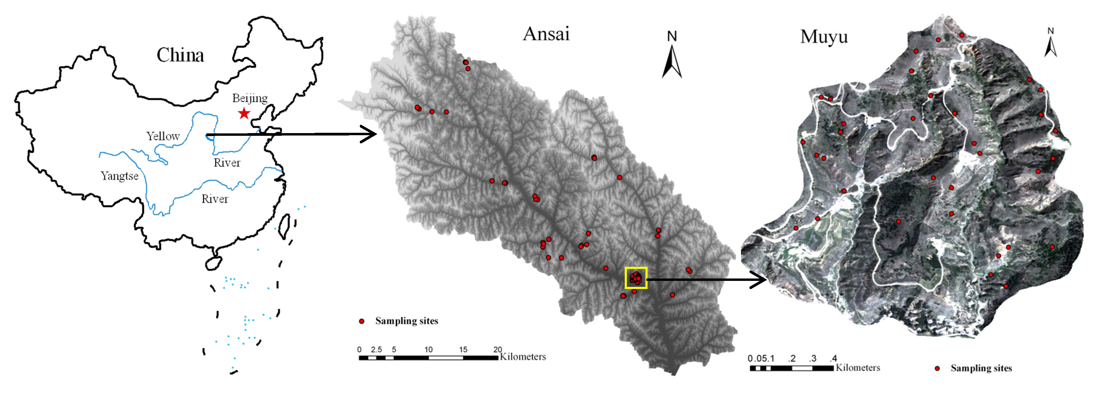
The Yanhe watershed lies in the middle of the Loess Plateau in the northern Shaanxi Province. The subwatershed in this study is located in the upstream section of the Yanhe and is controlled by a hydrometric station called “Ansai” (109°19′ E, 36°52′ N); as a matter of convenience, it is referred to as the Ansai watershed. The study area included the Ansai watershed (108°47′–109°25′ E, 36°52′–37°19′ N) and the Muyu small watershed (109°14.6′–109°15.5′ E, 36°58.9′–36°59.7′ N) (
Figure 1), which have an area of 1334 km
2 and 1.3 km
2, respectively. The study area has a very rugged topography, with an average slope of 23.9°: over 90% of the territory is composed of gullies and ridges, and the landform is a typical loess hilly-gullied landscape with elevations ranging from 1057 m to 1743 m above sea level, with an average of 1362 m. The area has a typical semiarid continental climate with an average temperature of 8.8 °C and an average annual precipitation of 505 mm. Rainfall shows high seasonal variability, with more than 60% of the annual precipitation occurring between July and September. The Ansai watershed is covered by a thick mantle of loess, an erosion-prone, fine silt soil. The percentage contents of different particle fractions are as follows: >0.25 mm (0.3%), 0.25–0.05 (18.7%), 0.05–0.01 (59%), 0.01–0.005 (6.2%), 0.005–0.001 (6.8%) and <0.001 (9%) [
25]. The Ansai watershed is located on a warm forest steppe, where natural forests have been destroyed. There were a large number of artificial plantings, predominantly
Robinia pseudoacacia and
Hippophae rhamnoides; the wild slope was covered with an herbaceous plant community that was composed mainly of
Artemisia gmelinii,
Artemisia giraldii,
Lespedeza davurica and
Stipa bungeana. There was garden plot planted mainly with apricot and pear trees. The cultivated crops were predominantly maize, millet and broom corn millet; these crops were in the booting stage, growing well at the date of sampling.
Figure 1.
Study area and location of the sampling points.
Figure 1.
Study area and location of the sampling points.
2.2. Experimental Design and Research Methods
In August 2012, we selected the Muyu small watershed as typical within the Ansai watershed by combining the current land use, water system, topographic and soil type maps in the study area used to survey the Ansai watershed. We took samples at 34 sites in the small watershed and at 76 sites for the watershed scale. The location of the study area and the distribution of sampling sites are indicated in
Figure 1. The number of sampling sites with respect to the land use type and location on the hill slope is shown in
Table 1.
The most important consideration for soil moisture research at the watershed scale is to determine how to lessen the effect of individual rainfall events on soil moisture content measurements. This will ensure that the data measured at different study sites are comparable. To further eliminate the influence of rainfall events on soil moisture content measurements, the soil moisture contents were measured 7 days after a rainfall event had occurred. We used a soil auger to drill to depths of 0–20 cm, 20–40 cm, 40–60 cm, 60–80 cm and 80–100 cm. We then measured the soil moisture using the oven-drying method. Three measurement points were collected for each sampling site. The distance between the 3 measurement points was more than 5 m, and the average soil moisture of the 3 points represented the soil moisture of the sampling site. We also used GPS (Trimble GeoExplorer 2008 Series GeoXH) to measure the latitude, longitude and elevation of the sampling sites. The difference between the elevation of the sampling sites and the watershed outlet was used to calculate the relative elevation. True north was 0 degrees, and aspect was the clockwise rotational angle and was measured using a compass. Slope was measured using a slope meter. Three people estimated the vegetation cover through observation according to the reference figure. The vegetation cover was calculated as the average of the 3 people’s visual measurements. The land use types and locations on the hill slope at the sampling sites were recorded.
Table 1.
Number of sampling sites with respect to land use type and location on the hill slope.
Table 1.
Number of sampling sites with respect to land use type and location on the hill slope.
| | | Small watershed scale | Watershed scale |
|---|
| Land use type | Shrubland | 4 | 10 |
| Woodland | 13 | 24 |
| Garden plot | 1 | 5 |
| Wild grassland | 13 | 22 |
| Cultivated land | 3 | 15 |
| Location on the hill slope | Slope top | 2 | 4 |
| Upper slope | 7 | 19 |
| Middle-upper slope | 8 | 11 |
| Middle slope | 7 | 14 |
| Middle-lower slope | 4 | 12 |
| Lower slope | 6 | 16 |
2.3. Data Analysis
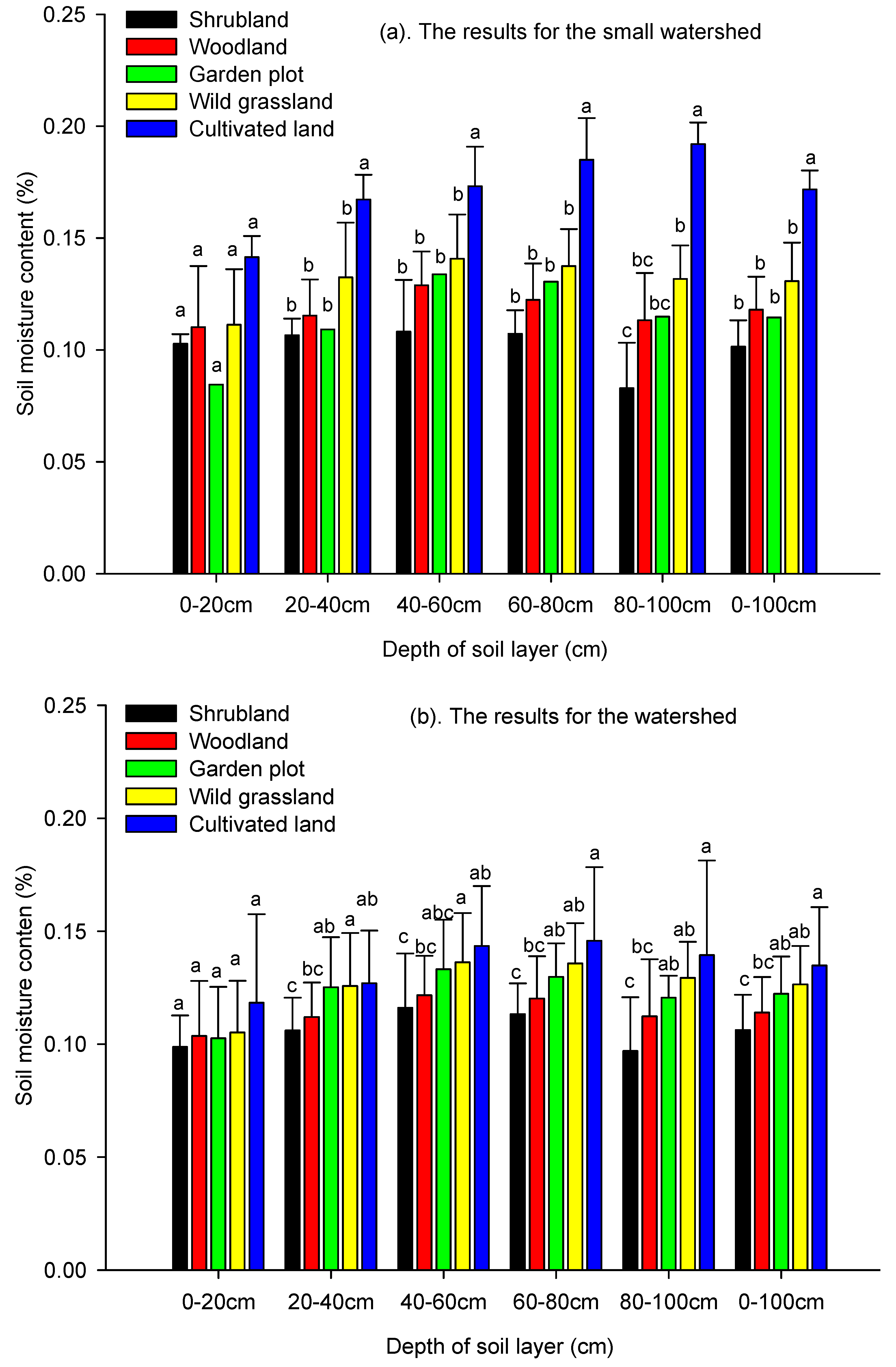
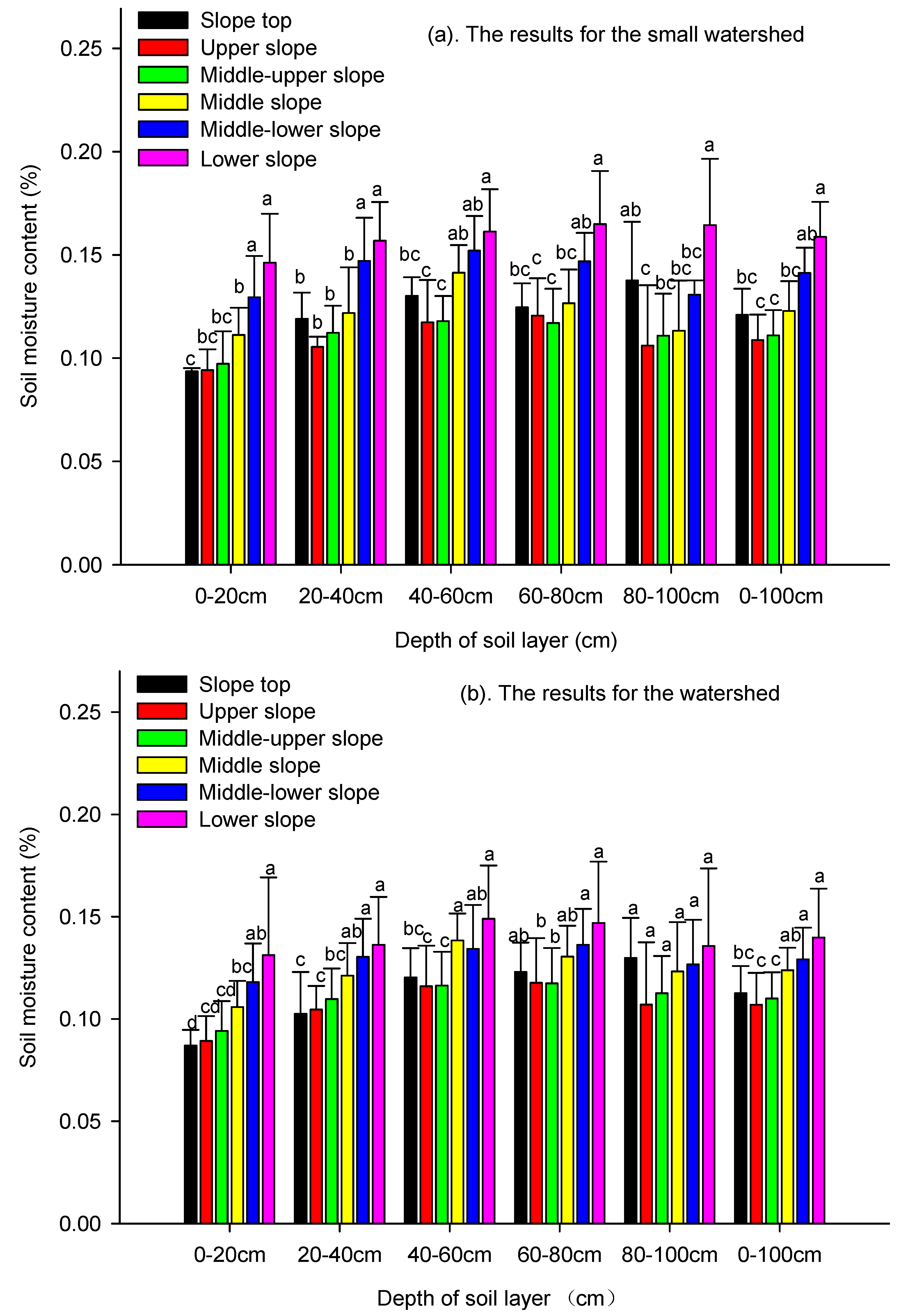
We completed a Pearson correlation analysis between soil moisture and aspect, relative elevation, slope and vegetation cover. We applied a general linear model (GLM) for a one-way analysis of variance (one-way ANOVA) and a Least-Significant Difference (LSD) method for multiple comparisons to analyze the influence of land use and location on the hill slope on soil moisture. We used the sampling sites as repetitions: the number of sampling sites was the number of repetitions, and thus, false repetition was avoided. All statistical analyses were based on the soil moisture date of the sampling sites, i.e., the average soil moisture of three measurement points at each sampling site.
The stepwise regression analysis selected variables that had a significant influence on the regression equations from among a large number of variables and eliminated the influence of possible multi-collinearity between factors in the interpretation of regression equations. The land use type and location on the hill slope were qualitative environmental factors that were converted into dummy variables for the general stepwise regression analysis. We used a 0–1 quantization process for the qualitative environmental factors. Shrubland was used as the reference category for land use type, so dummy variables were derived as follows: shrubland (A1 = 0, A2 = 0, A3 = 0, A4 = 0), garden plot (A1 = 1, A2 = 0, A3 = 0, A4 = 0), woodland (A1 = 0, A2 = 1, A3 = 0, A4 = 0), cultivated land (A1 = 0, A2 = 0, A3 = 1, A4 = 0), and wild grassland (A1 = 0, A2 = 0, A3 = 0, A4 = 1). The five land use types required four dummy variables, A1–A4, which represent “garden plot”, “woodland”, “cultivated land”, and “wild grassland”, respectively. The same approach was used for deriving the dummy variables of locations on the hill slope, where the middle-lower slope was used as the reference category.B1–B5 represent the “upper slope”, “lower slope”, “slope top”, “middle slope”, and “middle-upper slope”, respectively. With the other quantitative environmental variables, namely, the relative elevation, slope, sine of the aspect (indicating the east-west direction), cosine of the aspect (indicating the north-south direction) and vegetation cover, there were a total of 14 independent variables. We applied a stepwise regression analysis to determine the water moisture forecast model at different scales.


