Review

Quantifying the Relative Contributions of Forest Change and Climatic Variability to Hydrology in Large Watersheds: A Critical Review of Research Methods

1
Earth and Environmental Science Department, University of British Columbia (Okanagan), 3333 University Way, Kelowna BC V1V 1V7, Canada
2
College of Landscape and Art, Jiangxi Agricultural University, No.1101, Zhi Min Road, Nanchang 330045, China
3
Institute of Ecology and Environmental Science, Nanchang Institute of Technology, No. 289, Tianxiang Road, Nanchang 330099, China
*
Author to whom correspondence should be addressed.
Water 2013, 5(2), 728-746; https://doi.org/10.3390/w5020728
Submission received: 1 April 2013 / Revised: 20 May 2013 / Accepted: 21 May 2013 / Published: 13 June 2013
(This article belongs to the Special Issue Ecological Watershed Management)

Abstract

:
Forest change and climatic variability are two major drivers for influencing change in watershed hydrology in forest–dominated watersheds. Quantifying their relative contributions is important to fully understand their individual effects. This review paper summarizes the progress on quantifying the relative contributions of forest or land cover change and climatic variability to hydrology in large watersheds using available case studies. It compared pros and cons of various research methods, identified research challenges and proposed future research priorities. Our synthesis shows that the relative hydrological effects of forest changes and climatic variability are largely dependent on their own change magnitudes and watershed characteristics. In some severely disturbed watersheds, impacts of forest changes or land use changes can be as important as those from climatic variability. This paper provides a brief review on eight selected research methods for this type of research. Because each method or technique has its own strengths and weaknesses, combining two or more methods is a more robust approach than using any single method alone. Future research priorities include conducting more case studies, refining research methods, and considering mechanism-based research using landscape ecology and geochemistry approaches.

1. Introduction

Studies on the relationship between forests and water in forested watersheds have been conducted over the last century. Researchers have provided reviews at different times [1,2,3,4,5,6]. The general conclusions are that forest removal increases annual mean flow, peak flow and base flow when soils are not significantly disturbed. This relationship can be reversed if forest change is associated with soil compaction and decreased infiltration [7]. However, the majority of these conclusions is from the studies conducted in small watersheds, usually less than 100 km2, and cannot simply be extrapolated to large watersheds (more than 1000 km2). This suggests that more studies on the relationship between forest change and water in large watersheds must be conducted separately. In large watersheds, research targeting the relationship between forest changes and water is limited. There are many reasons contributing to fewer large watershed studies. The first and perhaps the most important reason is that paired watershed approach is not suitable for large watersheds because of the difficulty of locating reference watersheds with similar climate, vegetation and topography. The second reason is that large watersheds have different land uses and their complex interactions. Additionally, large watersheds very rarely coincide with the long-term records of hydrology, land use, and climate that exist for smaller research watersheds. However, with the expanding scope of land use planning and environmental protection, resource managers and planners require appropriate information at large watersheds or landscapes to support management decisions. Therefore, large watershed studies are urgently needed.
It has been widely accepted that climate variability and land cover or land use changes are two critical drivers for influencing watershed hydrological changes. Because of this, it is important to separate their relative contributions to hydrological change so that their individual effects can be quantified. In small watersheds, a paired watersheds approach is usually used to remove the effect of climate variability so that the effects of forest or land cover changes can be quantitatively assessed. However, this experimental paired watersheds approach is generally not feasible for large watersheds. Thus, alternative methods must be used for studying this subject in large watersheds. In the past 20–30 years, researchers have developed and applied diverse techniques for this research subject. These techniques can be broadly classified into statistical and modeling (process-based watershed modeling) categories. The objectives of this review are: (1) to describe various existing research methods and compare their pros and cons; (2) to briefly summarize the progress on quantifying the relative contributions of forest or land cover change and climatic variability to hydrology in large watersheds using available case studies; and (3) to identify research challenges and propose future research priorities.

2. Research Methods

2.1. Hydrological Modeling

Hydrological models are frequently used in the large watershed hydrological research. Hydrological models can be divided into lumped, semi-distributed and fully-distributed models. Lumped hydrological models study the watershed as a whole, and do not consider the detailed, spatial representations of watershed elements and processes. Unlike lumped or semi-distributed models, distributed models can well represent a watershed by assigning input data and physical characteristics to grids or elements. Physically based distributed models are able to provide distributed approximations or predictions of hydrological variables across watersheds, and thus have a better representation of reality. However, a fully-distributed model requires a large dataset with data on various processes, components and their interactions. For a large-scale watershed research, a semi-distributed model is commonly used because of a general absence of detailed data at large scales.
The one-factor-at-a-time approach (OFAT) commonly used in sensitivity analysis [8,9,10] is also used in association with hydrological models to distinguish the impact of climate factors and land cover change on watershed hydrology [11,12]. In a hypothetical example, the impacts of climatic variability and land use change on runoff are assessed with the available data in the period of 1960 to 2000. First, we keep the land cover in 1960 unchanged over the simulation period while climate change is allowed from 1960 to 2000. Then we simulate the runoff change (ΔQC), which can be treated as the impact of climatic variability on hydrology. Second, keep the climate of 1960 unchanged while land cover is changed, then calculate the runoff change (ΔQL) as the impact of land cover change. Finally, we assume the changes of both climate and land cover, then calculate the runoff change (ΔQL + C). In this way, the relative contributions of forest and land cover changes and climatic variability to hydrology can be computed.
Various distributed hydrological models have been successfully used to quantitatively study the effects of climate change and forest change/land cover change on hydrology, for examples, SWAT [13,14], DHSVM [15,16,17], MIKE-SHE [18], etc. In spite of increased applications, hydrological models are still based on our current theories that are deeply rooted in the physics of small-scale processes. This gives rise to difficulties in representing nonlinear hydrological processes and their interactions at all scales across heterogeneous landscapes. In addition, calibrating and testing a model may not always assure its validity, since there are some inherent drawbacks in the approaches of parameter calibration and validation. We often over-parameterize our models to meet high accuracy levels, ignoring the equifinality problem that different parameter sets for a model might yield the same result during calibration, but distinctly different predictions when conditions are altered [19,20].

2.2. Trend Analysis

Trend analysis is a commonly used method to qualitatively assess hydrologic responses [21,22,23,24]. The trend analysis uses historic data to fit a curve, which reflects a trend of the interested hydrological variable and can then be used to predict any future values if the trend is statistically significant.
Water 05 00728 i001
Water 05 00728 i002
Water 05 00728 i003
where the Equation (1) is used to calculate the slope of a time series data; the Equation (2) is used to estimate change percentages of the sample mean E(x); and the Equation (3) is for correlation coefficient at a significant level.
When the trend analysis is applied to detect the effects of forest change on hydrology, information on climate change and land use change is needed. If there is no a significant trend in climate variable (e.g., precipitation), the significant trend in hydrological variable is then judged to be caused by forest change or land cover change [24,25]. Clearly, this method is simple and qualitative, but may not be reliable, as the interactions between forest change and climatic variability are not considered. Wei and Zhang detected the offsetting effects of forest change and climatic variability on annual streamflow, which caused an insignificant trend on annual mean flow even though the forest effects on hydrology were statistically significant [26].

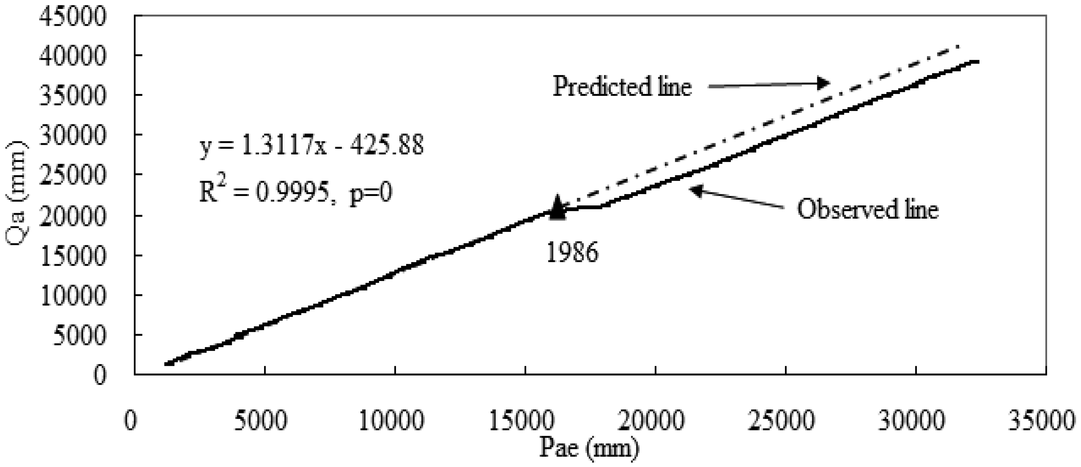
2.3. Double Mass Curves

Double Mass Curve (DMC) is a simple and intuitive method, widely used in long-term trend analysis of hydrometeorological elements. DMC draws a curve between two cumulative hydro-meteorological variables to test the consistency of two variables or analyze the trend change and its strength [27,28,29,30]. DMC method can be also used to separate the relative influences of forest change and climatic effects to hydrology [31]. For example, a modified DMC (MDMC) between cumulative annual streamflow and cumulative effective precipitation (the difference between total precipitation and evapotranspiration) is constructed for a large forested watershed (Figure 1). In this way, climatic effect on annual streamflow can be eliminated. In the period of no forest disturbance, the curve should produce a straight line, a baseline that describes the linear relation between annual streamflow and annual effective precipitation, and a break in this curve (e.g., year 1986 in Figure 2) would suggest the change of annual streamflow caused by forest disturbance. In other words, a step change or regime shift occurs in the slope of MDMC and the slope before the break is different from that afterwards. However, this visually detected breakpoint needs confirmation of its statistical significance by a non-parametric test or application of ARIMA model [32,33]. The difference between actual observations and the predict line after the change point can be calculated, and is regarded as the cumulative impact of forest changes.

2.4. Quasi-Paired Watershed Method

Paired watershed method compares two adjacent basins with similarity in size, morphology, geology, climate and vegetation including one as control and the other as treatment. The method is widely used in studying forest-water relationship in small (<100 km2) watersheds. For large watersheds, the concept of “quasi-paired watersheds” was proposed [34]. The quasi-paired watersheds method chooses two or more basin, with relative similarity in size, morphology, geology, climate and vegetation, but different forest disturbance levels. In this method, the watershed experienced the least forest disturbance is treated as “control”. Double mass curves of runoff coefficients (annual runoff/precipitation) obtained by plotting accumulated coefficients of the “treated” (Ct) against those of the “control” watershed (Cc), are used to detect the effect of forest disturbance on annual mean flow. If the “treated” watershed undergoes insignificant disturbance, a straight line would be expected. Otherwise, a break in the observed line indicates the emerging effect of forest disturbances on a hydrological variable (e.g., annual mean flow), and the difference between the expected and observed lines can be attributed to the difference in forest disturbances between “control” and “treated” watersheds. Statistical significance of the breakpoint found in the DMC slope can be tested using ARIMA intervention analysis [35,36].
Figure 1. A hypothetical example of application of the MDMC (modified double mass curve) between cumulative annual runoff (Qa) and cumulative annual effective precipitation (Pae) for assessing the effects of forest change on annual mean flow.
Water 05 00728 g001
Figure 2. Relationship between forest or land cover changes (LUCC) and their relative contributions to streamflow.
Water 05 00728 g002
The method is an alternative approach to the paired watersheds method where there are two similar watersheds with contrasted forest disturbance levels or land use changes. If long-term data are available, such a method can provide reliable results as what the paired experimental watersheds do. The challenge of this method is that it requires the “treated” watershed must have two significant long periods with and without severe forest disturbance. In addition, both watersheds should have relative similarity in climate, soil and vegetation. This could impose some difficulties in large watersheds where great spatial heterogeneities and complexities always exist.

2.5. Sensitivity-Based Approach

Sensitivity-based approach is similar to elasticity method [37], and is used to calculate the effect of climate variability on streamflow. Perturbations in both precipitation and PET can lead to changes of water balance. It can be assumed that a change in mean annual runoff can be determined using the following expression [31,38]:
ΔQclim = βΔP+γΔPET
where ΔQclim, ΔP, and ΔPET are changes in streamflow, precipitation, and potential evapotranspiration, respectively, and β and γ are the sensitivity coefficients of streamflow to precipitation and potential evapotranspiration, expressed as:
Water 05 00728 i004
Water 05 00728 i005
where x is the mean annual index of dryness (equal to PET/P); and the values of vegetation factor w for forest, grassland and shrub land are 2, 0.5 and 1, respectively [39].
This method is suitable for the analysis of a single basin, and for quantitative calculation of the impact of climate variables on runoff. Once the effects of climatic variability on flow are estimated, the effects of forest disturbance or land use changes can be deducted from total streamflow variations. The method has been successfully used for several case studies [37,38,39]. There may be two challenges in this method. First, it is not easy to determine w values for specific forest vegetation types. Where there are always different types of forests in a large watershed, how to select a specific w value remains challenging. Second, the effect of forest disturbance or land use changes on hydrology is indirectly estimated from total hydrological variations and the effects of climatic variability. Thus, its reliability is dependent on the accuracy of the other two terms.

2.6. Simple Water Balance

The water balance methods provide a framework to determine changes in the water balance components [40]. Simple water balance model can be used to determine the influence of climate and vegetation on streamflow at a watershed scale.
P = ET + Q + ΔS
where P is precipitation, ET is actual evapotranspiration, Q is streamflow and S is change in catchment water storage. When averaged over a long period, deep percolation (recharge) and change in soil moisture storage is often only 5% to 10% of the annual water balance, and therefore the change in catchment water storage (ΔS) can be neglected [41,42].
Precipitation and actual evapotranspiration constitute the most important variables to influence runoff change at the watershed scale. Precipitation, which varies both in temporal trend and spatial distribution, is regarded as independent of vegetation types [39], which mainly reflects changes of climate. However, actual evapotranspiration is a complex process. There are various ways to estimate watershed-scale evapotranspiration. For example, following the Budyko’s hypothesis, the simple two-parameter model for estimating the actual evapotranspiration was developed [43,44]. The model is consistent with the previous theoretical work and shows good agreement with more than 250 catchment-scale measurements from around the world [39,45,46].
Water 05 00728 i006
where ET is the actual evapotranspiration, ET0 is reference evapotranspiration as substitute of potential evapotranspiration calculated by the P-M method. The w is the plant-available water coefficient estimated in the same way as in the sensitivity-based approach [39].
The following steps were used to describe how a simple water balance method is implemented to estimate the effects of forest change on hydrology [40]. They are described as follows. First, according to Equation (8), calculate the actual evapotranspiration using the original data including precipitation, air temperature, relative humidity, wind speeds and sunshine hours after calculating ET0 by the P-M method. Second, estimate annual runoff using the Equation (10). In this step, the change of annual runoff is influenced by both climate variability and vegetation changes, and thus, the calculated annual runoff can be defined as Qv + C; Third, removing the decreasing or increasing trend of precipitation, air temperature, relative humidity, wind speeds and sunshine hours in data series to make them as stationary time series [47], recalculate the ET0 using the detrended climate variables and estimate annual runoff according to the Equations (10) and (11). In this step, the change of annual runoff mainly reflects the influences of vegetation changes, and thus, the recalculated annual runoff can be defined as Qv. Finally, calculate the difference between Qv + C and Qv so the change of annual runoff caused by the climate variability can then be estimated [40].
A simple water balance method provides a new way to distinguish the impact of climatic variables and vegetation factors on hydrological change. However, the choice of w values and the difficulty associated with removal of the decreasing or increasing trends in climate data may introduce some errors in this method.

2.7. Time Trend Method

In the time trend method, a relationship is established between discharge and climatic variables before the basin’s vegetation perturbation occurs and is then used to predict the discharge response of post-perturbation assuming undisturbed basin conditions. The typical time trend approach is to divide the whole study period into the calibration section and prediction section. The model accuracy depends on the length of the calibration or pre-perturbation periods [48].
During the calibration section:
Q1 = aP1 + b
During the forecast section:
Q2 = aP2 + b
Water 05 00728 i007
where P is precipitation, Q is runoff, Qʹ is the predicted streamflow for the treated catchment (from using Equation (9) developed during the calibration period), ΔQveg represents the change in mean annual streamflow because of vegetation change, subscripts 1 and 2 represent the calibration period and the prediction period, and b is the fitted regression coefficient.
This method uses a simple regression to express the relationship between precipitation and runoff both before and after forest cover changes. The method only requires data of precipitation, runoff and other meteorological variables, and the requirement on the detailed forest cover change can be ignored to some extent. The method may accept discontinuous data. Depending on different hydrometeorological characteristics in a study basin, time trend method performance at yearly hydrological variables is better than on the variables at monthly or daily intervals. Guardiola-Claramonte et al. proposed to consider the impact of temperature on the relationship between precipitation and runoff [49].

2.8. Tomer-Schilling Framework

Tomer and Schilling developed an elegant, coupled water–energy balance framework that requires long-term time series of precipitation (P), streamflow (Q), and PET to assess if unused available energy and water were related to climate and/or to land management in agricultural catchments [25,50]. The conceptual framework that qualitatively discriminates whether the dominant drivers of observed changes are related to land cover change and/or climate. The framework relating changes in land cover change and/or climate to the observed changes in the excess amounts of water (Pex) and excess amounts of energy (Eex) as fractions is illustrated in Peña-Arancibia et al. [25].
The Tomer–Schilling framework assumes that land cover change will affect ET but not P or PET, acknowledging that effects of land cover change on P and PET can be considered indirect at this scale and of second order when compared to changes in ET in the woodland environment. Thus, land cover change will cause ecohydrological shifts towards increased Pex and Eex, or towards decreased Pex and Eex. Changes in climate are required to cause increased Pex and decreased Eex, due to the temporal increase in the P/PET ratio and vice versa [25].
Water 05 00728 i008
Water 05 00728 i009
Tomer-Schilling framework is an effective and qualitative analysis tool of hydrological processes. The method can not only analyze long-term impacts of climate and forest cover on hydrology, but also explain the main factors of hydrological responses in different time periods. However, as all the qualitative methods, the impact of each variable of climate or vegetation cannot be quantitatively evaluated, and this brings difficulties to study the common law of hydrological responses under different topographies and different vegetation types.

3. Research Progress

Table 1 summarizes the progress on quantifying the relative contributions of climate variability and forest or land cover changes to hydrology in large watersheds. As shown in Table 1, more researchers have used statistical methods, while the others have applied the modeling approach. There are two reasons contributing to this difference. First, statistical methods normally analyze historic data for assessing the effects of forest change and climate variability, while models predict the possible effects of future scenarios on hydrology. With increasing availability of long-term data on hydrology, climate and land use change, it is not surprising that statistical methods gain more popularity due to their efficiency and provision of robust inferences. Hydrological models can be used to simulate the relative contributions of forest change and climate variability to hydrology, but they are limited due to the lack of various empirical relationships at large watersheds. Second, data on forest change or land over change are difficult to collect at large spatial scales across extended time periods. Without these data, models are difficult to calibrate. In comparison, some statistical methods such as trend analysis method, sensitivity-based approach and the elasticity method [51,52,53,54,55] can be used to quantify the effects of climatic variability first and then estimate the influence of forest or land cover change from the total variations. Those estimations can be done without long-term data on forest or land cover changes. However, in the watersheds where long-term and high quality data are not available for application of statistical approaches, models can be alternative approaches given that there are sufficient data for model calibration and validations.
Among the applied models (Table 1), SWAT, a semi-distributed model was widely used to evaluate the effects of climate and land use changes on streamflow [56,57]. It simulated streamflow responses to change in climate, land use, or both to distinguish the impact of climate variability from that of land use change on hydrology [35,58,59]. Other distributed hydrological models such as DTVGM model (Distributed Time-Variant Gain Model); VIC model (Variable Infiltration Capacity) and DHSVM model (Hydrology-Soil-Vegetation Model) were also applied to this research topic (Table 1). For example, lumped hydrological model (CHARM) and distributed model (TOP MODEL) were used to simulate the effect of climate variability and land cover change on hydrology in the upper reaches of the Yangtze River [58]. Three applied models show similar results, suggesting that their simulations were reliable.
There is a clear tendency that a combined approach of two or more complementary techniques (particularly the combination of statistical and modeling methods) is superior to application of a single technique alone. For example, both climate elasticity and hydrological modeling methods were applied to distinguish the effects of climate variability and human activities in Baiyangdian Basin [52]. Using the climate elasticity method, the results indicated that climate variations accounted for 40% of decrease in streamflow, while human activities accounted for 60%. Using the hydrological modeling method, the results showed that climate variations accounted for 38% of decrease in streamflow, while human activities accounted for 62%. Because two independent methods achieved relatively consistent results, the result was believed more reliable.
The general perception is that climate is dominant in influencing streamflow change [26,60,61]. However, Table 1 shows that the relative hydrological effects of climate variability and forest change or land use change are largely dependent on their own change magnitudes and watershed characteristics. In some severely disturbed watersheds, impacts of forest change or land cover change are as important as those from climate change. For example, large-scale land use changes and practices were found to be the most important factor responsible for the streamflow change in the northwest China’s Loess Plateau (Table 1) [21,40]. Based on comparable studies listed in the Table 1, we detected that a significant linear relationship between forest or land cover changes and their contributions to streamflow changes (Figure 2). This significant linear relationship clearly demonstrated that the more severe change of forest or land cover, the greater in their relative contributions to hydrological changes. Another example showed that the forest disturbance (25%–30%) accounted for 45% of decrease in streamflow and is similar to that from climate change (55%) in Willow watershed located in the central interior of British Columbia, Canada [26].
Table 1. Summary of the studies on relative contributions of forest or land cover changes and climate variability to hydrology.
MethodWatershed (km2)Forest change or land use change (%) at a watershed Relative contribution (%)References
Climate variabilityForest change/land use change
Hydrological ModelingThe source regions of Yellow River (1.22 × 10⁵ km2)0.13%~34.03% area change in woodland and shrub/grassland65%–95%6%–16%[56]
Heihe River watershed (1506 km2)4.5% of the catchment area was changed mainly from shrubland and sparse95.8%9.6%[57]
Suomo Watershed (2536 km2)Forest area decreased by 17%, open woodland increased by 8%, grassland area increased by 10%60%–80%20%[62]
Hydrological ModelingThe upper Yangtze River watershed (13,721~1,005,501 km2)Human activities55%–73.3%28.5%–46.7%[63]
Chaobai River watershed (57,001 km2)Human activities34%64%[64]
Araguaia River watershed, Brazil (385,000 km2)55% Deforestation33%67%[65]
Trend AnalysisShiyang river watershed (389~1614 km2)Area change in Forest, crop and grassland64.5%–87.9%12.1%–35.5%[66]
Hun–Tai River watershed (1112~11,203 km2)Human activities43%57%[67]
Pyrenees Watershed, Spain (3.25 × 10⁴ km2)The increase of agricultural land70%30%[68]
Wuding River watershed (30,261 km2)43% (The soil conservation measures)13%87%[45]
Qingshui River watershed (436 km2)Cropland decreased by 72.1%, woodland increased by 963.60% and residential area increased by 576.07%46.79%53.21%[69]
Taoer River watershed (41,600 km2)Paddy field increased by 2%, upland increased by 15.10%, forest decreased by 10.60%45%55%[61]
ColumbiaRiver watershed, Canada (385,000 km2)Human activities48%–55%45%–52%[70]
Double Mass CurvesThe Willow River watershed, Canada (2,860 km2)19.7% Deforestation55%45%[26]
The Upper Zagunao River watershed (2528km2)15.5% Deforestation42.5%57.5%[71]
Quasi-paired Watershed MethodYulin, 8.28 km2 Xinlin, 28 km2Forest cover increased from 20% to 80%/8.61%[30]
Sensitivity-Based ApproachUpper catchment of the Yellow River Watershed (222,551 km2)Human activities50%40%[55]
Baiyangdian Lake (3,465 km2)Construction of water conservation facilities38%–40%60%–62%[52]
The headwaters of the Yellow River Watershed (1.32 × 10⁵ km2)Water and soil conservation engineering30%70%[72]
Sensitivity-Based ApproachThe Loess Plateau (1,279–9,289 km2)Water and soil conservation engineering21%–57%43%–79%[21]
Crawford River watershed, Darlot Creek watershed, Tinana Creek watershed (698–1,174 km2)Afforestation 13.4%–23.5%21%–49%61%–64%[73]
Simple Water BalanceYiluo River watershed (1.89 × 10⁵ km2)Water and soil conservation engineering21.75%78.26%[40]
Time Trend MethodSeven paired catchments from Australia, New Zealand, and South Africa (0.18–3.44 km2)Clearing vegetation 32%–100% Afforestation 67%–83% Forest conversion 100%10%–72%28%–98%[55]
The upper reach of the Weihe River (1.35 × 10⁵ km2)Human activities40%60%[64]
Plata watershed, Paragury(3.2 × 10⁴ km2)Forest land converted to cropland41%–53%51%–59%[74]
Tomer-Schilling FrameworkFour candidate Midwest watershedsChanges in agricultural land coverIncrease/decreased Pex and EexIncreased Pex and decreased Eex[50]

4. Future Research Challenges and Research Priorities

As mentioned previously, all methods summarized in this paper can be classified into two categories: statistics and simulation. The statistical methods normally provide robust inference about the relationship between hydrological responses and forest change or land cover changes. However, those methods treat a study basin as a black box, and rarely involve the mechanisms or processes. On the other hand, the simulation methods, especially fully-distributed models consider the hydrological processes and their interactions, but due to the lack of data and various empirical relationships in large watersheds, the model calibration and validation are often time consuming and inaccurate. Therefore, it is logical to believe that the combination of statistical methods and modeling can complement their strengths and overcome their shortcomings, and thus could be an improved research strategy.
Forest disturbance and climate change are considered to be the two main drivers interactively affecting the hydrological changes in large watersheds (Figure 3). Climate change can affect hydrology directly due to its influence on precipitation and temperature. Climate change can also affect hydrology in an indirect way. For example, more forest fires and pests can be induced by drought, and these forest disturbances in turn affect the hydrological processes. In an opposite way, vegetation can change evapotranspiration and thus streamflow. They can also affect hydrology indirectly. For example, vegetation types and distributions may affect the characteristics of air humidity, temperature, precipitation, and consequently hydrological cycle. As far as we know, the literature is extremely limited on that topic, with some pioneering examples exploring the interactions among forest change, climate and hydrological responses [75,76].
In addition, current studies mainly focused on the changes in annual runoff, with less emphasis on peak and low flows. Assessing the relative contributions of forest or land cover changes and climatic variability to the change in peak and low flows is likely more challenging and may require separate methods such as geochemistry and landscape ecology in large watersheds. The isotope method in geochemistry could help analyze the sources (surface water, groundwater, glacier melt water, etc.) and flow pathways in the watersheds, while landscape ecology or geoscience allows us to examine the role of watershed configuration and topographic characteristics in the effects of the forest or land cover changes on hydrology [7,51,77,78,79,80,81]. However, such research is needed to support resource management decisions for protection of watershed functions and public safety in large watersheds or regions.
Figure 3. A conceptual framework showing interactions among climate change, forest change and hydrological responses.
Water 05 00728 g003
Here, we propose the following future research priorities in this subject. First, more case studies are needed. Assessing the relative contributions of forest or land cover changes and climatic variability to hydrology is rather limited in large watersheds. Zhang and Wei compared two adjacent large watersheds located in the interior of British Columbia, and found the contrasted conclusions under the similar forest disturbance levels [35]. They further concluded that the effects of forest change on hydrology in large watersheds are likely watershed specific. This clearly demonstrates that more case studies are needed before generally conclusions can be derived. Second, a research priority should be given on improvement of research methods. Although quite a few research methods are currently available for studying the impacts of forest change and climate change on hydrology, there is no a commonly-accepted method. The lack of commonly-accepted methods may limit our ability to compare the results of different studies. Third, in large watershed studies, analytical results are largely based on data quality and spatial coverage. Large spatial variations in precipitation, temperature, solar radiation, humidity, wind speed, surface albedo, canopy characteristics, etc. in these large watersheds constraint our ability to derive robust conclusions. Future studies should be designed to specifically address uncertainties. Finally, more research should be on mechanisms and processes. It is difficult to study the mechanisms and processes in large watersheds, mainly due to lack of the suitable methodology and data for assessing the complicated interactions and cumulative behaviors across various spatial scales. However, such research is critical for explaining and verifying the findings obtained through statistical and modeling approaches.

Acknowledgments

This work was financially supported by the National Science Foundation of China (No. 31170665) and theYoung Scientific Funding of Nanchang Institute of Technology (2012KJ004).

Conflicts of Interest

The author declares no conflict of interest.

References

  1. Andreassian, V. Waters and forests: From historical controversy to scientific debate. J. Hydrol. 2004, 291, 1–27. [Google Scholar] [CrossRef]
  2. Bosch, J.M.; Hewlett, J.L. A review of catchment experiments to determine the effects of vegetation changes on water yield and evapotranspiration. J. Hydrol. 1982, 55, 3–23. [Google Scholar] [CrossRef]
  3. Hibbert, A.R. Forest Treatment Effects on Water Yield. In Proceedings of International Symposium on Forest Hydrology, Fort Collins, CO, USA, 6–8 September 1967; Sopper, W.E., Lull, H.W., Eds.; p. 813.
  4. Jackson, R.B.; Jobbágy, E.G.; Avissar, R.; Roy, S.B.; Barrett, D.J.; Cook, C.W.; Farley, K.A.; le Maitre, D.C.; McCarl, B.A.; Murray, B.C. Trading water for carbon with biological carbon sequestration. Science 2005, 310, 944–1947. [Google Scholar]
  5. MacDonald, L.H.; Stednick, J.D. Forests and Water: A State-of-the-Art Review for Colorado; CWRRI Completion Report No. 196; Colorado Water Resources Research Institute, Colorado State University: Fort Collins, CO, USA, 2003. [Google Scholar]
  6. Price, K. Effects of watershed topography, soils, land use, and climate on baseflow hydrology in humid regions: A review. Progr. Phys. Geogr. 2011, 35, 465–492. [Google Scholar] [CrossRef]
  7. Price, K.; Jackson, C.R.; Parker, A.J.; Reitan, T.; Dowd, J.; Cyterski, M. Effects of watershed land use and geomorphology on stream low flows during severe drought conditions in the southern Blue Ridge Mountains, Georgia and North Carolina, USA. Water Resour. Res. 2011, 47, W02516. [Google Scholar]
  8. Gao, X.; Sorooshian, S.; Gupta, H.V. Sensitivity analysis of the biosphere-atmosphere transfer scheme. J. Geophys. Res. 1996, 101, 7279–7289. [Google Scholar] [CrossRef]
  9. Pitman, A.J. Assessing the sensitivity of a land-surface scheme to the parameter values using a single column method. J. Clim. 1994, 7, 1856–1869. [Google Scholar] [CrossRef]
  10. Wilson, M.F.; Henderson-Sellers, A.; Dickinson, R.E.; Kennedy, P.J. Sensitivity of the Biosphere-Atmosphere Transfere Scheme (BATS) to the inclusion of variable soil characteristics. J. Appl. Meteorol. Climatol. 1987, 26, 341–362. [Google Scholar] [CrossRef]
  11. Wilson, M.F.; Henderson-Sellers, A.; Dickinson, R.E.; Kennedy, P.J. Investigation of the sensitivity of the land-surface parameterization of the NCAR Community Climate Model in regions of tundra vegetation. Climatology 1987, 7, 319–343. [Google Scholar] [CrossRef]
  12. Karvonen, T.; Koivusalo, H.; Jauhiainen, M.; Palko, J.; Weppling, K. A hydrological model for predicting runoff from different land use areas. J. Hydrol. 1999, 217, 253–256. [Google Scholar] [CrossRef]
  13. Zhang, A.J.; Zhang, C.; Fu, G.B.; Wang, B.D.; Bao, Z.X.; Zheng, H.X. Assessments of impacts of climate change and human activities on runoff with swat for the Huifa River Basin, northeast China. Water Resour Manage 2012, 26, 2199–2217. [Google Scholar] [CrossRef]
  14. Chen, J.F.; Li, X.B.; Zhang, M. Simulating the impacts of climate variation and land-cover changes on basin hydrology: A case study of the Suomo Basin. Sci. China Ser. D 2005, 48, 1501–1509. [Google Scholar] [CrossRef]
  15. Cuo, L.; Giambelluca, T.W.; Ziegler, A.D. Lumped parameter sensitivity analysis of a distributed hydrological model within tropical and temperate catchments. Hydrol. Process. 2011, 25, 2405–2421. [Google Scholar] [CrossRef]
  16. Sun, W.Y.; Bosilovich, M.G. Planetary boundary layer and surface layer sensitivity to land surface parameters. Boundary Lay. Meteorol. 1996, 77, 353–378. [Google Scholar] [CrossRef]
  17. Stonesifer, C.S. Modeling the cumulative effects of forest fire on watershed hydrology: A post-fire application of the Distributed Hydrology-Soil-Vegetation Model (DHSVM). J. Hydrol. 2007, 10, 282–290. [Google Scholar]
  18. Christiaens, K.; Feyen, J. Analysis of uncertainties associated with different methods to determine soil hydraulic properties and their propagation in the distributed hydrological MIKE SHE model. J. Hydrol. 2001, 246, 63–81. [Google Scholar] [CrossRef]
  19. Beven, K. The future of distributed models: Model calibration and uncertainty prediction. Hydrol. Process. 1992, 6, 279–298. [Google Scholar] [CrossRef]
  20. Kirchner, J.W. Getting the right answers for the right reasons: Linking measurements, analyses, and models to advance the science of hydrology. Water Resour. Res. 2006, 42, W03S04. [Google Scholar] [CrossRef]
  21. Zhang, X.P.; Zhang, L.; Zhao, J. Responses of stream flow to changes in climate and land use/cover in the Loess Plateau, China. Water Resour. Res. 2008, 44, W00A07. [Google Scholar]
  22. Sheng, Y.; Michio, H. Statistical interpretation of the impact of forest growth on stream flow of the Sameura Basin, Japan. Environ. Monit. Assess. 2005, 104, 369–384. [Google Scholar] [CrossRef]
  23. Wilcox, B.P.; Huang, Y. Woody plant encroachment paradox: Rivers rebound as degraded grasslands convert to woodlands. Geophys. Res. Lett. 2010, 37, L07402. [Google Scholar]
  24. Zhou, G.Y.; Wei, X.H.; Luo, Y.; Zhang, M.F.; Li, Y.; Qiao, Y.; Liu, H.; Wang, C. Forest recovery and river discharge at the regional scale of Guangdong Province, China. Water Resour. Res. 2010, 46, W09503. [Google Scholar]
  25. Peña-Arancibia, J.L.; van Dijk, A.I.J.M.; Guerschman, J.P.; Mulligan, M.; Bruijnzeel, L.A.; McVicar, T.R. Detecting changes in stream flow after partial woodland clearing in two large catchments in the seasonal tropics. J. Hydrol. 2012, 416–417, 60–71. [Google Scholar]
  26. Wei, X.H.; Zhang, M.F. Quantifying stream flow change caused by forest disturbance at a large spatial scale: A single watershed study. Water Resour. Res. 2010, 46, W12525. [Google Scholar]
  27. Buttle, J.M.; Metcalfe, R.A. Boreal forest disturbance and stream flow response, northeastern Ontario. Can. J. Fish. Aquat. Sci. 2000, 57, 5–18. [Google Scholar] [CrossRef]
  28. Siriwardena, L.; Finlayson, B.L.; McMahon, T.A. The impact of land use change on catchment hydrology in large catchments: The Comet River, Central Queensland, Australia. J. Hydrol. 2006, 326, 199–214. [Google Scholar] [CrossRef]
  29. Wigbout, M. Limitations in the use of double mass curves. J. Hydrol. 1973, 12, 132–138. [Google Scholar]
  30. Yao, Y.F.; Cai, T.J.; Wei, X.H.; Zhang, M.F.; Ju, C.Y. Effect of forest recovery on summer streamflow in small forested watersheds, Northeastern China. Hydrol. Process. 2011, 26, 1208–1214. [Google Scholar]
  31. Koster, R.D.; Suarez, M.J. A simple framework for examining the interannual variability of land surface moisture fluxes. J. Clim. 1999, 12, 1911–1917. [Google Scholar] [CrossRef]
  32. Box, G.; Cox, D. An analysis of transformations, J.R. Stat. Soc. B 1964, 26, 211–252. [Google Scholar]
  33. Box, G.; Pierce, D. Distribution of residual autocorrelations in autoregressive integrated moving average time series models. J. Am. Stat. Assoc. 1970, 65, 1509–1526. [Google Scholar] [CrossRef]
  34. Buttle, J.M. Identifying Hydrological Responses to Basin Restoration: An Example from Southern Ontario. In Watershed Restoration Management: Physical, Chemical, and Biological Considerations; McDonnell, J.J., Stribling, J.B., Neville, L.R., Leopold, D.J., Eds.; American Water Resources Association: Herndon, VA, USA, 1996; pp. 5–13. [Google Scholar]
  35. Zhang, M.F.; Wei, X.H. The effects of forest disturbance on hydrology in two contrasted watersheds. Hydrol. Processes. 2013. submitted for publication. [Google Scholar]
  36. Zhang, M.F.; Wei, X. Alteration of flow regimes caused by large-scale forest disturbance: A case study from a large watershed in the interior of British Columbia, Canada. Ecohydrology 2013, in press. [Google Scholar]
  37. Dooge, J.C.I.; Bruen, M.; Parmentier, B. A simple model for estimating the sensitivity of runoff to long–term changes in precipitation without a change in vegetation. Adv. Water Resour. 1999, 23, 153–163. [Google Scholar]
  38. Jones, R.N.; Chiew, F.H.S.; Boughton, W.C.; Zang, L. Estimating the sensitivity of mean annual runoff to climate change using selected hydrological models. Adv. Water Resour. 2006, 29, 1419–1429. [Google Scholar] [CrossRef]
  39. Zhang, L.; Dawes, W.R.; Walker, G.R. The response of mean annual evapotranspiration to vegetation changes at catchment scale. Water Resour. Res. 2001, 37, 701–708. [Google Scholar] [CrossRef]
  40. Liu, Q.; Yang, Z.F.; Cui, B.S.; Sun, T. Temporal trends of hydro-climatic variables and runoff response to climatic variability and vegetation changes in the Yiluo River Basin, China. Hydrol. Process. 2009, 23, 3030–3039. [Google Scholar] [CrossRef]
  41. Zhang, L.; Dawes, W.R.; Walker, G.R. Predicting the Effect of Vegetation Changes on Catchment Average Water Balance; Technical Report 99/12; Cooperative Research Centre for Catchment Hydrology. CSIRO Land and Water: Clayton South, Australia, 1999. [Google Scholar]
  42. Ponce, V.M.; Shetty, A.V. A conceptual-model of catchment water-balance: 1. Formulation and calibration. J. Hydrol. 1995, 173, 27–40. [Google Scholar] [CrossRef]
  43. Budyko, M.I. The Heat Balance of the Earth’s Surface; U.S. Department of Commerce: Dordrecht, The Netherland, 1958; p. 259. [Google Scholar]
  44. Budyko, M.I. Climate and Life; Academic Press: San Diego, CA, USA, 1974; p. 508. [Google Scholar]
  45. Li, L.J.; Zhang, L.; Wang, H.; Wang, J.; Yang, J.W.; Jiang, D.J.; Li, J.Y.; Qin, D.Y. Assessing the impact of climate variability and human activities on streamflow from the Wuding River Basin in China. Hydrol. Proces. 2007, 21, 3485–3491. [Google Scholar] [CrossRef]
  46. Zhang, L.; Hickel, K.; Dawes, W.R.; Chiew, F.H.S.; Western, A.W.; Briggs, P.R. A rational function approach for estimating mean annual evapotranspiration. Water Resour. Res. 2004, 40, W02502. [Google Scholar]
  47. Xu, C.Y.; Gong, L.B.; Jiang, T.; Chen, D.L.; Singh, V.P. Analysis of spatial distribution and temporal trend of reference evapotranspiration and pan evaporation in Changjiang (Yangtze River) catchment. J. Hydrol. 2006, 327, 81–93. [Google Scholar] [CrossRef]
  48. Zhao, F.F.; Zhang, L.; Xu, Z.X.; Scott, D.F. Evaluation of methods for estimating the effects of vegetation change and climate variability on streamflow. Water Resour. Res. 2010, 46, W03505. [Google Scholar]
  49. Guardiola-Claramonte, M.; Troch, P.A.; Breshears, D.D.; Huxman, T.E.; Switanek, M.B.; Durcik, M.; Cobb, N.S. Decreased streamflow in semi-arid basins following drought-induced tree die-off: A counter-intuitive and indirect climate impact on hydrology. J. Hydrol. 2011, 406, 225–233. [Google Scholar] [CrossRef]
  50. Tomer, M.D.; Schilling, K.E. A simple approach to distinguish land-use and climate-change effects on watershed hydrology. J. Hydrol. 2009, 376, 24–33. [Google Scholar] [CrossRef]
  51. Tootle, G.A.; Singh, A.K.; Piechota, T.C.; Farnham, I. Long lead-time forecasting of US streamflow using partial least squares regression. J. Hydrol. Eng. 2007, 12, 442–451. [Google Scholar] [CrossRef]
  52. Hu, S.S.; Zheng, H.X.; Liu, C.M.; Yu, J.J.; Wang, Z.G. Assessing the impacts of climate variability and human activities on streamflow in the water source area of Baiyangdian Lake. Acta Geograph. Sinica 2012, 67, 62–70. [Google Scholar]
  53. Zhang, L.; Zhao, F.F.; Chen, Y.; Dixon, R.N.M. Estimating effects of plantation expansion and climate variability on streamflow for catchments in Australia. Water Resour. Res. 2011, 47, W12539. [Google Scholar]
  54. Zhang, S.R.; Lu, X.X. Hydrological responses to precipitation variation and diverse human activities in a mountainous tributary of the lower Xijiang, China. Catena 2009, 77, 130–142. [Google Scholar]
  55. Zhao, F.F.; Xu, Z.X.; Zhang, L.; Zuo, D.P. Streamflow response to climate variability and human activities in the upper catchment of the Yellow River Basin. Sci. China Ser. E 2009, 52, 1–8. [Google Scholar]
  56. Chen, L.Q.; Liu, C.M. Influence of climate and land-cover change on runoff of the source regions of Yellow River. China Environ. Sci. 2007, 27, 559–565. [Google Scholar]
  57. Li, Z.; Liu, W.Z.; Zhang, X.C.; Zheng, F.L. Impacts of landuse change and climate variability on hydrology in an agriculture catchment on the Loess Plateau of China. J. Hydrol. 2009, 377, 35–42. [Google Scholar] [CrossRef]
  58. Guo, H.; Hu, Q.; Jiang, T. Annual and seasonal streamflow responses to climate and land-cover changes in the Poyang Lake Basin, China. J. Hydrol. 2008, 355, 106–122. [Google Scholar] [CrossRef]
  59. Hao, X.M.; Chen, Y.N.; Xu, C.C.; Li, W.H. Impacts of climate change and human activities on the surfaces runoff in the Tarim River Basin over the last fifty years. Water Resour. Manag. 2008, 22, 1159–1171. [Google Scholar] [CrossRef]
  60. Chen, J.F.; Li, X.B.; Zhang, M. Impacts of climate variability and land cover change on hydrology using model simulation in Suomuo Basin. Sci. China Ser. D 2004, 34, 668–674. [Google Scholar]
  61. Li, L.J.; Li, B.; Liang, L.Q.; Li, J.Y.; Liu, Y.M. Effect of climate change and land use on stream flow in the upper and middle reaches of the Taoer River, northeastern China. For. Stud. China 2010, 12, 107–115. [Google Scholar]
  62. Montenegro, S.; Ragab, R. Impact of possible climate and land use changes in the semi arid regions: A case study from North Eastern Brazil. J. Hydrol. 2012, 434–435, 55–68. [Google Scholar] [CrossRef]
  63. Xia, J.; Wang, M.L. Runoff changes and distributed hydrologic simulation in the upper reaches of Yangtze River. Resour. Sci. 2008, 30, 962–967. [Google Scholar]
  64. Wang, G.S.; Xia, J.; Wan, D.H.; Ye, A.Z. A Distributed monthly water balance model for identifying hydrological response to climate changes and human activities. J. Nat. Resour. 2006, 21, 86–91. [Google Scholar]
  65. Coe, M.; Latrubesse, E.; Ferreira, M.; Amsler, M. The effects of deforestation and climate variability on the streamflow of the Araguaia River, Brazil. Biogeochemistry 2011, 105, 119–131. [Google Scholar] [CrossRef]
  66. Ma, Z.M.; Kang, S.Z.; Zhang, L.; Tong, L. Analysis of impacts of climate variability and human activity on stream flow for a river basin in arid region of northwest China. J. Hydrol. 2008, 352, 239–249. [Google Scholar] [CrossRef]
  67. Zhang, Y.F.; Guan, D.X.; Jin, C.J.; Wang, A.Z.; Wu, J.B.; Yuan, F.H. Analysis of impacts of climate variability and human activity on streamflow for a river basin in northeast China. J. Hydrol. 2011, 410, 239–247. [Google Scholar] [CrossRef]
  68. Beguería, S.; López-Moreno, J.I.; Lorente, A.; Seeger, M.; García-Ruiz, J.M. Assessing the effect of climate oscillations and land-use changes on streamflow in the central Spanish Pyrenees. Ambio 2003, 32, 283–286. [Google Scholar]
  69. Tang, L.X.; Zhang, Z.Q.; Wang, X.J.; Wang, S.P.; Zha, T.G. Streamflow response to climate and landuse changes in Qingshui River watershed in the loess hilly-gully region of Western Shanxi Province, China. Chin. J. Plant Ecol. 2010, 34, 800–810. [Google Scholar]
  70. Naik, P.K.; Jay, D.A. Human and climate impacts on Columbia River hydrology and salmonids. River Res. Appl. 2011, 27, 1270–1276. [Google Scholar] [CrossRef]
  71. Zhang, M.F.; Wei, X.H.; Sun, P.S.; Liu, S.R. The effect of forest harvesting and climatic variability on runoff in a large watershed: The case study in the Upper Minjiang River of Yangtze River Basin. J. Hydrol. 2012, 464–465, 1–11. [Google Scholar] [CrossRef]
  72. Zheng, H.X.; Zhang, L.; Zhu, C.; Liu, C.M.; Sato, Y.; Fukushima, Y. Responses of streamflow to climate and land surface change in the headwaters of the Yellow River Basin. Water Resour. Res. 2009, 45, W00A19. [Google Scholar] [CrossRef]
  73. Li, H.Y.; Zhang, Y.Q.; Vaze, J.; Wang, B.D. Separating effects of vegetation change and climate variability using hydrological modelling and sensitivity-based approaches. J. Hydrol. 2012, 420–421, 403–418. [Google Scholar]
  74. Doylea, M.E.; Vicente, B.R. Attribution of the river flow growth in the Plata Basin. Int. J. Climatol. 2011, 31, 2234–2248. [Google Scholar] [CrossRef]
  75. Tague, C.; Grant, G.E.; Farrell, M.; Choate, J.; Jefferson, A. Deep groundwater mediates streamflow response to climate warming in the Oregon Cascades. Clim. Change 2008, 86, 189–210. [Google Scholar] [CrossRef]
  76. Van Wateren-de Hoog, B. A regional model to assess the hydrological sensitivity of medium size catchments to climate variability. Hydrol. Process. 1998, 12, 43–56. [Google Scholar] [CrossRef]
  77. Vivoni, E.R.; Entekhabi, D.; Bras, R.L.; Ivanov, V.Y. Controls on runoff generation and scale-dependence in a distributed hydrologic model. Hydrol. Earth Syst. Sci. 2007, 11, 1683–1701. [Google Scholar] [CrossRef]
  78. Tetzlaff, D.; Soulsby, C.; Waldron, S.; Malcolm, I.A.; Bacon, P.J.; Dunn, S.M. Conceptualization of runoff processes using a geographical information system and tracers in a nested mesoscale catchment. Hydrol. Process. 2007, 21, 1289–1307. [Google Scholar] [CrossRef]
  79. Christophersen, N.; Neal, C.; Hooper, R.P.; Vogt, R.D.; Andersen, S. Modeling streamwater chemistry as a mixture of soilwater end-members—A step towards 2nd-generation acidification models. J. Hydrol. 1990, 116, 307–320. [Google Scholar] [CrossRef]
  80. McGuire, K.J.; McDonnell, J.J. A review and evaluation of catchment transit time modeling. J. Hydrol. 2006, 330, 543–563. [Google Scholar] [CrossRef]
  81. Soulsby, C.; Tetzlaff, D.; Hrachowitz, M. Tracers and transit times: Windows for viewing catchment scale storage? Hydrol. Process. 2009, 23, 3503–3507. [Google Scholar] [CrossRef]

