Article

Factors Affecting Phosphorous in Groundwater in an Alluvial Valley Aquifer: Implications for Best Management Practices

1
Stockholm Environment Institute, US Center, 400 F Street, Davis, CA 95616, USA
2
Department of Biological Systems Engineering, Virginia Polytechnic Institute and State University, 33446 Research Drive, Painter, VA 23420, USA
3
Department of Biological and Environmental Engineering, Cornell University, 206 Riley-Robb Hall Ithaca, NY 14853, USA
4
Department of Land, Air and Water Resources, University of California at Davis, One Shields Avenue, Davis, CA 95616, USA
*
Author to whom correspondence should be addressed.
Water 2013, 5(2), 540-559; https://doi.org/10.3390/w5020540
Submission received: 19 February 2013 / Revised: 10 April 2013 / Accepted: 11 April 2013 / Published: 2 May 2013
(This article belongs to the Special Issue Ecological Watershed Management)

Abstract

:
Many streams in the US are impaired because of high Soluble Reactive Phosphorous (SRP) contributions from agriculture. However, the drivers of ecological processes that lead to SRP loss in baseflow from groundwater are not sufficiently understood to design effective Best Management Practices (BMPs). In this paper, we examine how soil temperature and water table depth influence the SRP concentrations in groundwater for a dairy farm in a valley bottom in the Catskills (NY, USA). Measured SRP concentrations in groundwater and baseflow were greater during the fall, when soil temperatures are warmer, than during winter and spring. The observed concentrations were within the bounds predicted by groundwater temperatures using the Arrhenius equation, except during fall, when concentrations rose above these predictions. These elevated concentrations were likely caused by mineralization and consequent accumulation of phosphorous (P) in summer. In addition, SRP concentrations were greater in near-stream areas, where water tables where higher. In short, SRP concentrations are dependent on temperature, demonstrating the importance of understanding the underlying mechanism of ecological processes. In addition, results suggest BMPs that apply manure on land having a deep groundwater, instead of on land with a shallow water table will lower overall SRP contributions.

1. Introduction

Many streams in the US are impaired due to elevated phosphorus (P) concentrations [1,2,3] that enter the stream via overland flow, subsurface flow and via point sources [4,5,6,7,8]. Agriculture is one of the main contributors and accounts for approximately half of the total P discharged into U.S. streams annually [9]. Especially in dairy-based agricultural systems, P is often applied to soils in excess of crop needs and therefore accumulates to problematic levels, whereby additional P cannot be effectively retained and becomes available for leaching with the soil solution [10]. To protect New York City’s water supply, located in the Catskill Mountains of New York State, the New York State Department of Environmental Conservation (NYSDEC) requires that reservoir P levels not exceed 20 μg L−1 [11]. As a result, Best Management Practices (BMPs) have been installed in order to control surface derived nutrient losses to water bodies (e.g., exclusionary fencing and cattle crossing [12], drainage ditch short circuiting [13], vegetative filter strips, [14,15] and other BMPs’ types [16,17,18,19,20,21]. Although recent research has shown that groundwater discharge can play a significant role in the loading of dissolved nutrients to surface water [22,23,24], limited research in the Catskill Mountains and elsewhere has been conducted on controlling Soluble Reactive Phosphate (SRP, or orthophosphate <45 µm) contributions from baseflow and groundwater [3,25,26,27].
Phosphorus concentration in baseflow and groundwater depends, among others things, on the water table depth with generally greater concentration occurring for shallow water tables than for deeper water tables, as noted by Obour et al. [28] and Martin et al. [29] in Florida, where the high concentrations resulted from the organic rich layers at the shallow depths. Scott et al. [30] found similar relationship between P concentrations and water table depth in the Catskills. In addition, SRP concentrations in streams may vary significantly with the time of year [31,32]. In the northeast US, concentrations are elevated during late summer and fall when temperatures are also elevated, and concentrations are low in late winter and early spring with low temperatures [33]. Temperature is the ecological driver and affects the anoxic conditions and rate constants of many chemical and microbiological reactions controlling the release of P to groundwater [34,35,36]. The Arrhenius equation has been used for simulating the temperature effects of the biotic and abiotic processes that describe the P loss [37,38,39,40,41,42,43].
In this paper we are interested in determining to what extent temperature (a driver of ecological processes) and groundwater table depth (resulting from landscape processes) affect SRP concentration in groundwater and in stream baseflow with the ultimate goal of finding ways to reduce contributions of P to baseflow by the use of specialized best management practices. To do this we will analyze a set of groundwater SRP data collected on a farm located on alluvial soils of the Catskill Mountains of Upstate New York.

2. Materials and Methods
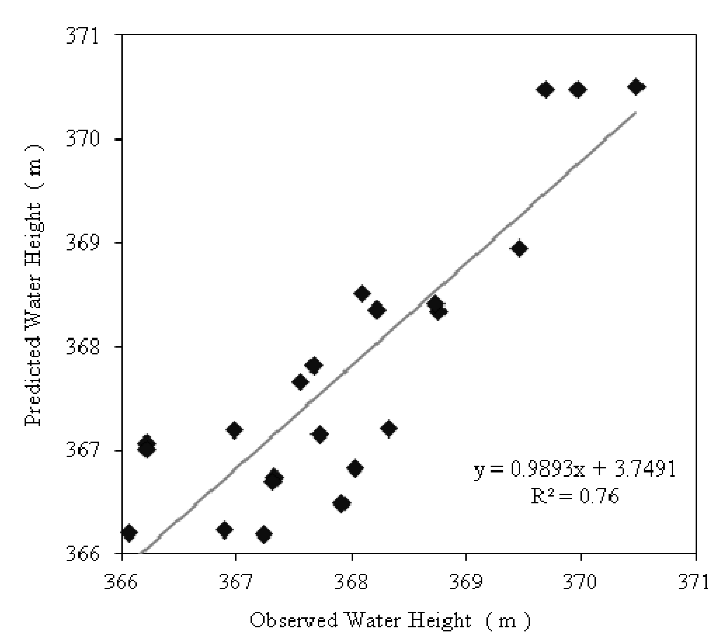
2.1. Study Site

The study was conducted from June 2004 through April 2006 on an alluvial valley plain in the Catskill Mountains of New York State (Figure 1). The 19 ha study site is located on a dairy farm in a valley bottom along a tributary of the West Branch of the Delaware River in the Cannonsville Reservoir watershed (1165 km2) that supplies drinking water to New York City [44]. It has a physiography characterized by narrow valleys with steep walls and flat valley bottoms. The depth to the groundwater table in the study site varies between zero and 1.0 m for much of the year. In the southern area of the study site, regional groundwater flow intersects the surface and forms saturated areas during October to May when precipitation exceeds evapotranspiration. A small creek originates from springs on the surrounding hills and drains into the main stream flowing from north-to-south (labeled as Creek B in Figure 1). Creek B is solely fed by baseflow from groundwater and was used for stream sampling.
Figure 1. Location of the study area within the Catskills mountains, and the location of the piezometers.
Water 05 00540 g001
Soils are classified in the Barbour-Trestle complex (coarse-loamy-skeletal over sandy or sandy-skeletal mixed, active, mesic Fluventic Dystrudepts). The principal water-bearing material is Pleistocene sand and gravel [45]. Overland flow is typically absent because of the high infiltration rates of these alluvial soils. Depth to the bedrock is approximately 18 m based on a measurement taken from a nearby well located 1 km to the north [44]. The climate of the study site is humid continental with an average temperature of 8 °C. The average annual precipitation is 112 cm year−1 [46] one-third of which falls as snow. The growing season is from May to September. The nearest weather station is located in Walton, 9 km to the southeast of the field site.
The monitoring site is located on a farm that encompasses 19 ha of valley bottom land parallel to the stream and 119 ha of uphill lands (not shown in Figure 1) dominated by deciduous forest. Of the 19 ha of valley bottom land, 10 ha is managed as corn and 9 ha as pasture. In June 2005 the land use changed in the southern area of the farm on approximately 4 ha, from pasture to corn land for the remainder of the study. Rotation follows a three year cycle of Alfalfa and corn. The farm has 60 adult dairy and beef cows and 36 heifers producing 833 Mg (ton) of manure annually. The farm does not have any manure storage so the manure is generally handled and applied daily as a solid and milkhouse wastewater is sometimes added to it for its disposal. In the winter about eighty percent of the manure is spread on the valley bottom lands (average rate of 35 Mg ha−1). During the growing season the herd primarily grazes in the pastures and manure is randomly deposited, and any remaining manure from the barn and milkhouse wastewater is spread less frequently as needed. The farm has participated in whole farm planning since September 1995 as part of the Watershed Agricultural Program established by the New York City Department of Environmental Protection (NYCDEP), the New York State Department of Environmental Conservation (NYSDEC), the Watershed Agricultural Council (WAC), and the Environmental Protection Agency (EPA).
Soil samples taken in the field around the farm in 2004 showed that total P concentrations were above the levels that indicate of high P accumulation in the soil [12].

2.2. Groundwater Sampling

To measure water table heights and facilitate groundwater sampling, 22 subsurface PVC piezometers were installed at depths ranging from 0.3 to 1.5 m in the southern field of the study site (Figure 1) [44]. The piezometers were 3.5 cm in diameter; with a screened length of 0–0.3 m from the bottom and wrapped with geosynthetic filter cloth. Piezometers were closed at the bottom and were installed by auguring a hole with a diameter slightly larger than the piezometer. The piezometers were then sealed with bentonite to exclude overland flow from entering the piezometer. A total of 542 groundwater samples were drawn from the piezometers from July 2004 to April 2006. Capacitance probes (TruTrack Inc, Christchurch, New Zealand) were installed adjacent to the piezometers to measure the groundwater table height on 1 h intervals at 1 mm resolution.

2.3. Stream Sampling

A total of 146 stream water samples were taken at four locations (B1, B2, B3, and B4) along the course of Creek B. B1 was the spring of the creek and sampling points B2, B3, and B4 were located 65, 130, and 200 m downstream, respectively. Sampling site B4 was located directly upstream from the confluence with the main stream. More information about stream water quality data and analysis are given in [12]. Piezometers and Creek B were sampled on the same day at 15-day-intervals. Sampling dates were grouped by season for data analysis.

2.4. Water Chemistry Analysis

Groundwater and stream flow samples were collected at least bimonthly from June 2004 through April 2006. At each sampling time, 100 mL samples were collected using a peristaltic pump rinsed with distilled water before each use. Piezometer purging was done prior to sample collection. The pump’s output tube was kept in the sampling bottle for the entire pumping duration to allow the groundwater to be well mixed, and to minimize water contact with ambient air during pumping. Water samples were collected with no headspace and stored in coolers for transport to the laboratory. Water samples were filtered through 0.45 μm membrane filters using a vacuum pump filtering system, and the filtered samples were analyzed for SRP within 24 h of sampling, or were stored at 4 °C until analysis. The samples were analyzed using the OI Analytical FlowSystem 3000 Automated Ascorbic Acid Method for SRP with a detection limit of 0.001 mg L−1 [Method 4500-P G (Ortho-P) and Method4500-Ph (Total P)] [47].

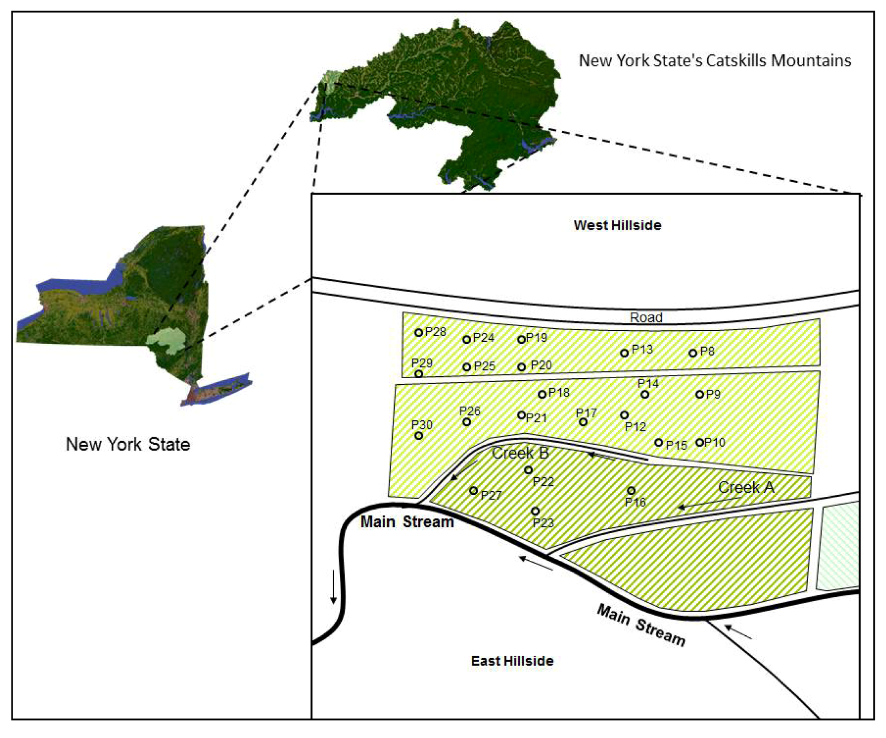
2.5. Modeling of Ground Water Flow and Streamlines

The groundwater table heights were measured at 22 locations paired with the sampling piezometers (Figure 1), and the capacitance probe elevations were referenced to a common elevation with a laser survey. The groundwater flow direction was determined based on the measured water table heights using Visual MODFLOW. Both streamlines and groundwater flow were determined for average steady state flow conditions over almost two years from 6 June 2004 to 30 April 2006 based on observed groundwater table heights.
The boundary conditions for the MODFLOW model consisted of a constant head boundary at the northern edge obtained from the capacitance probes installed adjacent to piezometers P8, P9, and P10 (Figure 1). The capacitance probes measured vertical variations in the water table height intercepting the groundwater flux coming from upstream areas. For the southern edge a constant head boundary was defined at the surface water level elevation of the main stream (Figure 1). The stream course and the shallow bedrock layer along the western hillside were used to define the eastern and western edge boundaries, respectively, as no-flow boundaries. Depth to bedrock was assumed to be 18 m for the valley bottom between both the eastern and western hillslopes based on the nearby well borehole and landscape observations. The model was calibrated by varying the saturated hydraulic conductivity and the constant head boundaries to obtain the best fit to the observed water table heights averaged over the 672 days period.

2.6. Spatial Analysis of Ground Water SRP

To obtain a spatial pattern of groundwater SRP, the log transformed average measured groundwater SRP concentrations in spring, summer, fall, and winter were evaluated were interpolated with ordinary kriging using the Geostatistical Analyst extension in ArcMap 9.2 [48]. Cross-validation was used to evaluate spatial modeling errors [48]. The prediction errors that were measured during the cross-validation include: mean, root-mean-square (RMS), average standard, mean standardized, and RMS standardized.

2.7. Predicting Temperature Effect on SRP Concentrations

The temperature effects on SRP concentrations were simulated similar to Hively et al. [49] using an Arrhenius type of equation [38,41,43]:
Water 05 00540 i001
where Cw is the SRP export coefficient (mg L−1), corresponding to the average predicted SRP concentration in baseflow, T is the temperature of the soil where the baseflow is originating from (°C), Tref is the reference temperature (°C) at which the reference concentration, Cref, was estimated (mg L−1) as the value that best fit the model, and X the factor change (range 1 to 5) for a 10 °C change in temperature (see also Table 3). Hively et al. [49] obtained a good fit for observed and predicted SRP values in the Catskill’s using X = 2.5.
The soil temperature (T) in Equation (1) at a depth z (m) was calculated assuming that the annual surface temperature varies as a sine wave [50,51]:
Water 05 00540 i002
where Water 05 00540 i003 
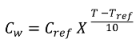
is the damping depth (m) described by Dt, the soil’s thermal diffusivity (m2 d−1) and ω = 2π/365 the radial frequency (d−1), Ta the annual average air temperature (°C), A0 is annual amplitude of the air temperature (°C), and t0 a lag time so that when t0 days have passed (starting at t = 0) the air temperature is equal to the average air temperature, i.e., T(t0, 0) = Ta.

3. Results and Discussion

3.1. Precipitation

The partial years sampled during this study had approximately normal precipitation levels [12]. The average precipitation during the growing season (May to September) and the non-growing season were 596 mm and 661 mm, respectively [46]. A considerable difference was observed between the 2004 and 2005 growing seasons, where 829 mm of precipitation was measured in 2004 but only 311 mm during the 2005 growing season. The two non-growing seasons (October to April of 2004–2005 and of 2005–2006, respectively) had precipitation slightly above average, 722 and 751 mm, respectively. Temperature was normal all years, with the strongest deviation in average temperature being in 2005, which was 1 degree above average.

3.2. Groundwater Flow and Streamlines

Water table height across the study area increased and decreased at approximately the same rate during the study period (with the exception of a few piezometers close to the stream and at the southern area). At these locations, the groundwater table reached the surface during large storms. Thus, since the groundwater gradients changed minimally during the course of the year, we used a steady state MODFLOW model to determine groundwater flow. The hydraulic conductivity was used as calibration parameter for obtaining a good fit. The fit using a saturated conductivity of 10 m day−1 between the calibrated state and observed average water table height was satisfactory with an R2 = 0.76 (p-value <0.001) (Figure 2). Overall, the groundwater table surface followed the ground surface elevation with horizontal hydraulic gradients of approximately 0.01.
Figure 2. Comparison of observed water heights measured using piezometers versus predicted water heights modeled using MODFLOW.
Water 05 00540 g002
The calibrated equipotential lines for the groundwater and the streamlines for the 22 piezometers are shown in Figure 3. The streamline for P21 had the shortest travel distance (30 m) before reaching Creek B, and P8 had the longest travel distance (420 m) to the main stream water course (Figure 3). Streamlines indicated that only nine of the 22 piezometers influenced Creek B (P10, P12, P15, P17, P18, P21, P22, P27, and P30 in Figure 3) under average state groundwater flow. Although there were some piezometers (e.g., P14 and P26 in Figure 3) located at a relatively short perpendicular distance from Creek B, streamlines of these piezometers indicated that they did not influence Creek B.
The groundwater flow’s average linear velocity was estimated using Darcy’s Law. Taking the calibrated saturated hydraulic conductivity, Ks, of 10 m day−1 used by the groundwater flow model, an average hydraulic gradient, dh/dl, of 0.01, and an estimated porosity of 0.4; a calculated groundwater flow velocity was approximately 0.25 m day−1, or 90 m year−1. Hence, the estimated groundwater travel time from P21, which had the shortest travel distance (30 m) to Creek B, is in the order of 100 days and the most distant point is (420 m) is five years.
Figure 3. Map of groundwater table based on equipotential lines for the average state groundwater flow conditions over a period of 672 days showing the streamlines output for the 22 piezometers. The shadow area is a polygon mask applied to the 380 m by 500 m grid design and it is delineated by the corresponding eastern and western edge boundaries, a straight line in the northern edge, and an open ditch on the southern edge joining the main stream water course.
Water 05 00540 g003

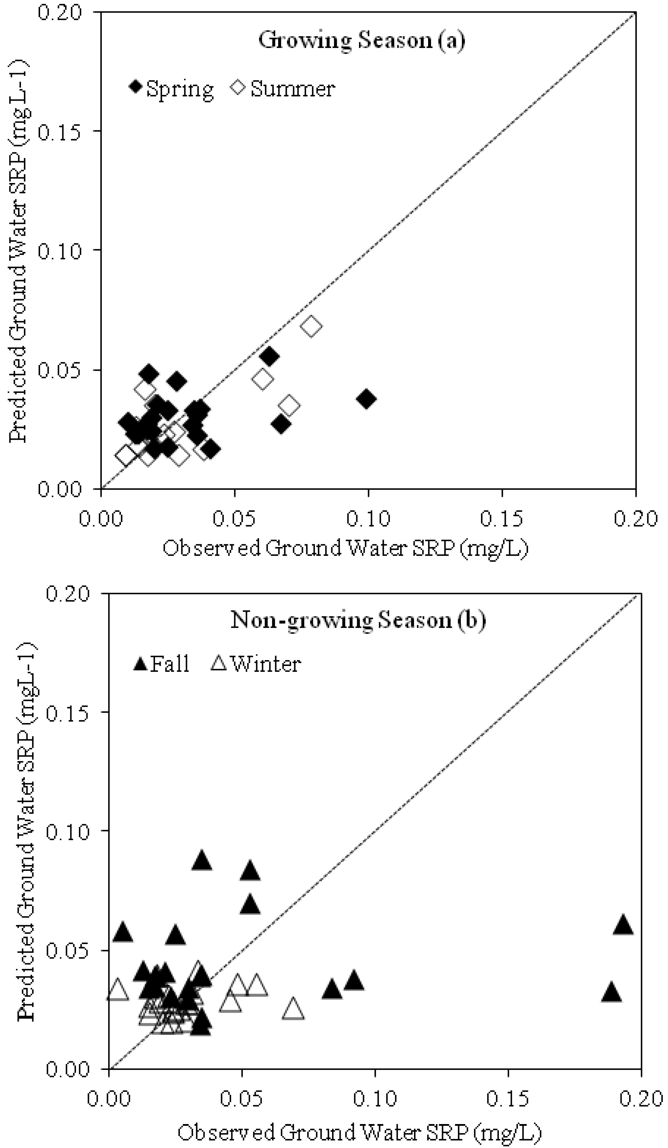
3.3. Groundwater and Stream Flow SRP Concentrations

Overall groundwater and baseflow concentrations were similar and around 0.035 mg L−1 with concentration greatest during the fall and lowest during spring (Table 1). Minimum concentrations observed in baseflow during summer and spring, were around 0.01 mg L−1 and less than 0.005 mg L−1 during fall and winter (Table 1). During high flow events maximum concentrations were significantly greater in the baseflow of Creek B and the groundwater because the groundwater came close to the ground surface where P concentrations were greater [44]. In these cases surface water table intersected with the ground likely contributing to the elevated concentrations in Creek B. Groundwater SRP concentrations are similar to those reported by Young and Briggs [52] for agricultural fields and riparian areas in central New York State.
Table 1. Descriptive statistics of SRP values for all piezometers placed in the study area (including those that were not used for this paper), and those feeding Creek B, and Creek B stream flow. All SRP data in mg L−1.
SeasonSites (n)Samples (n)Minimum SRPMaximum SRPMean SRPMedian SRPS.E. of MeanSkewness
All Piezometers Placed in the Study Area
Spring221480.0100.0990.0320.0250.0051.93
Summer16880.0090.0820.0290.0190.0051.43
Fall221760.0050.1930.0480.0320.0112.25
Winter221300.0030.0690.0280.0240.0031.23
Piezometers Feeding Creek B
Spring9590.0140.0750.0280.0190.0092.56
Summer7380.0140.0820.0340.0200.0111.11
Fall9720.0050.1860.0510.0350.0192.15
Winter9550.0030.0620.0260.0220.0061.75
Creek B Stream Flow
Spring4310.0080.1750.0240.0140.0054.52
Summer4420.0060.2390.0350.0280.0064.73
Fall4470.0020.3970.0460.0150.0112.97
Winter4260.0020.1610.0440.0270.0091.47

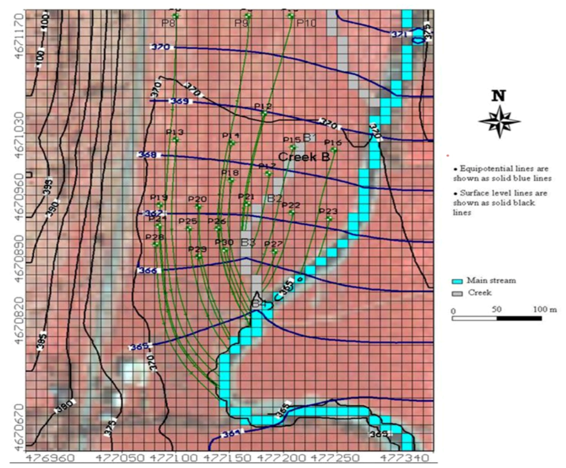
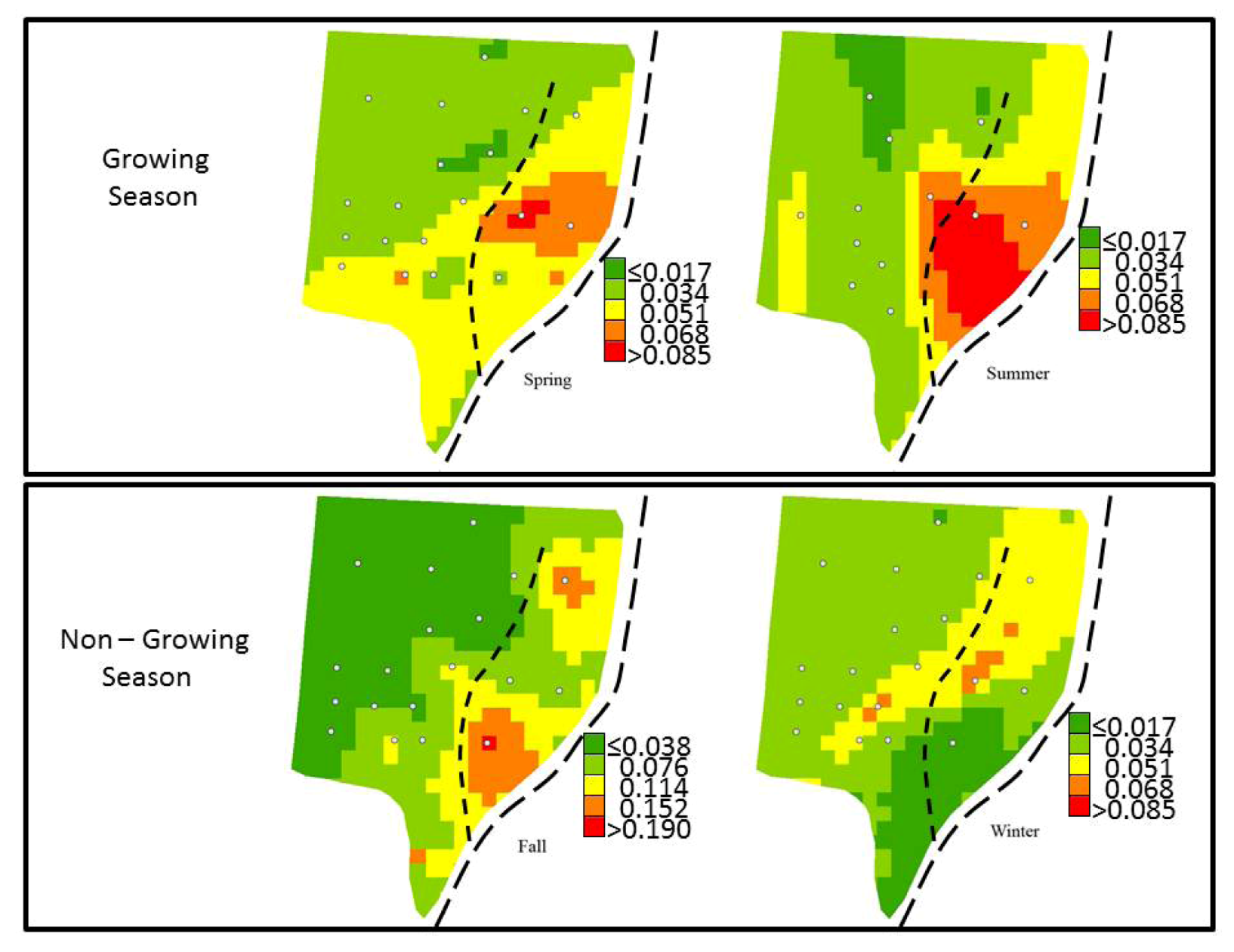
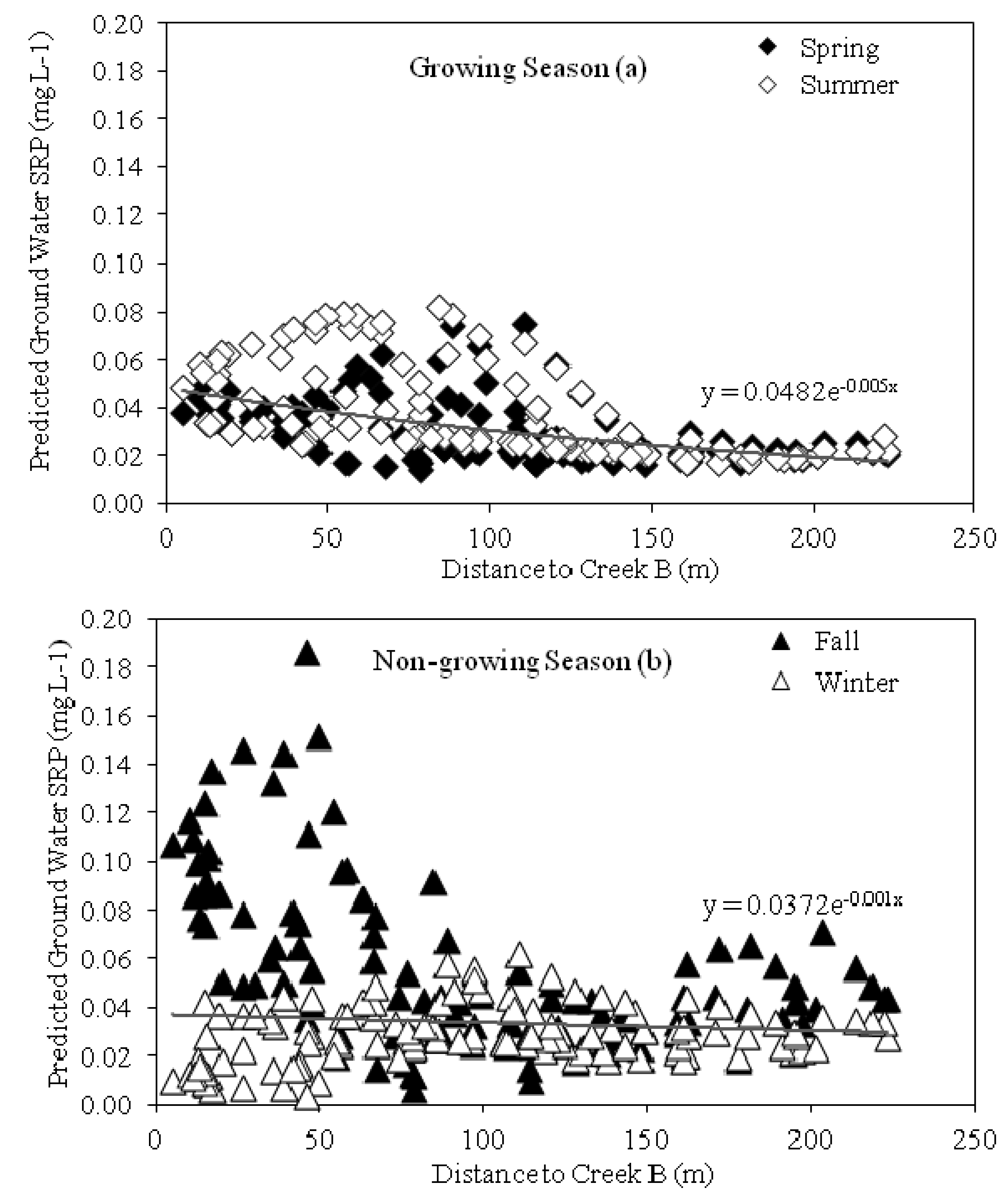
3.4. Spatial Variability of Groundwater SRP

Two seasonal maps describing the growing season (spring, summer), and two maps describing the non-growing season (fall, winter) were created with kriging using log-transformed groundwater SRP data. The estimated seasonal groundwater SRP concentration maps at 10-m resolution are shown in Figure 4. Distinct spatial patterns emerge where the greatest estimated concentrations were identified during the non-growing season of fall in the area near Creek B and the confluence with the main stream water course. Concentrations ranged from 0.007 mg L−1 in the north- and southeastern area, up to 0.19 mg L−1 in some localized areas between Creek B and the main stream water course (Figure 4). This spatial distribution indicates that the area susceptible to greater groundwater SRP concentrations is located in the downstream area of Creek B between the creek itself and the main stream water course.
The estimated groundwater SRP concentrations in Figure 4 based on a kriging interpolation of the observed data groundwater are deemed to be acceptable. The cross-validation results for this analysis are summarized in Table 2 whereby the mean predicted SRP errors are close to zero and the RMS standardized errors are near unity, with the results relatively similar across all four seasons.
More observations would have generated more robust estimations as indicated by the mean standardized errors being slightly larger than mean errors. Nevertheless, the scatter plot of observed versus the predicted SRP values shown in Figure 5 are clustered around the 1:1 line, although there are some outliers particularly for the fall season. Regression slopes for the spring, summer, fall, and winter, were 0.71, 0.80, 0.46, and 0.83 respectively, indicating some under prediction. This is likely due to the kriging method that uses average data based on distances to known concentrations, and can therefore not predict the outliers (high concentrations due to preferential flow).
Figure 4. Estimated groundwater Soluble Reactive Phosphorous (SRP) concentration maps for the spring, summer, fall and winter. Spring, summer and winter maps have the same concentration scale for predicted values (mg L−1), while the fall map does not. White dots represent the piezometers locations at the field site, the short dashed line represents Creek B, and the longer dashed line is the main stream course.
Water 05 00540 g004
Table 2. Mean predicted SRP concentrations and error values by season for the groundwater maps in Figure 3.
SeasonMean Predicted SRPRoot-Mean-Square ErrorAverage Standard ErrorMean Standardized ErrorRoot-Mean-Square Standardized Error
Spring−0.001580.019700.02171−0.115700.9522
Summer−0.001030.014510.02051−0.127300.7551
Fall−0.003970.051560.06982−0.132100.8944
Winter0.000720.014730.02335−0.040360.7134
Figure 5. Observed versus predicted groundwater SRP (mg L−1) for the growing (a); and non-growing seasons (b). During the fall and spring seasons, several data points were observed away from the 1:1 line, indicating an under-prediction of SRP concentrations.
Water 05 00540 g005

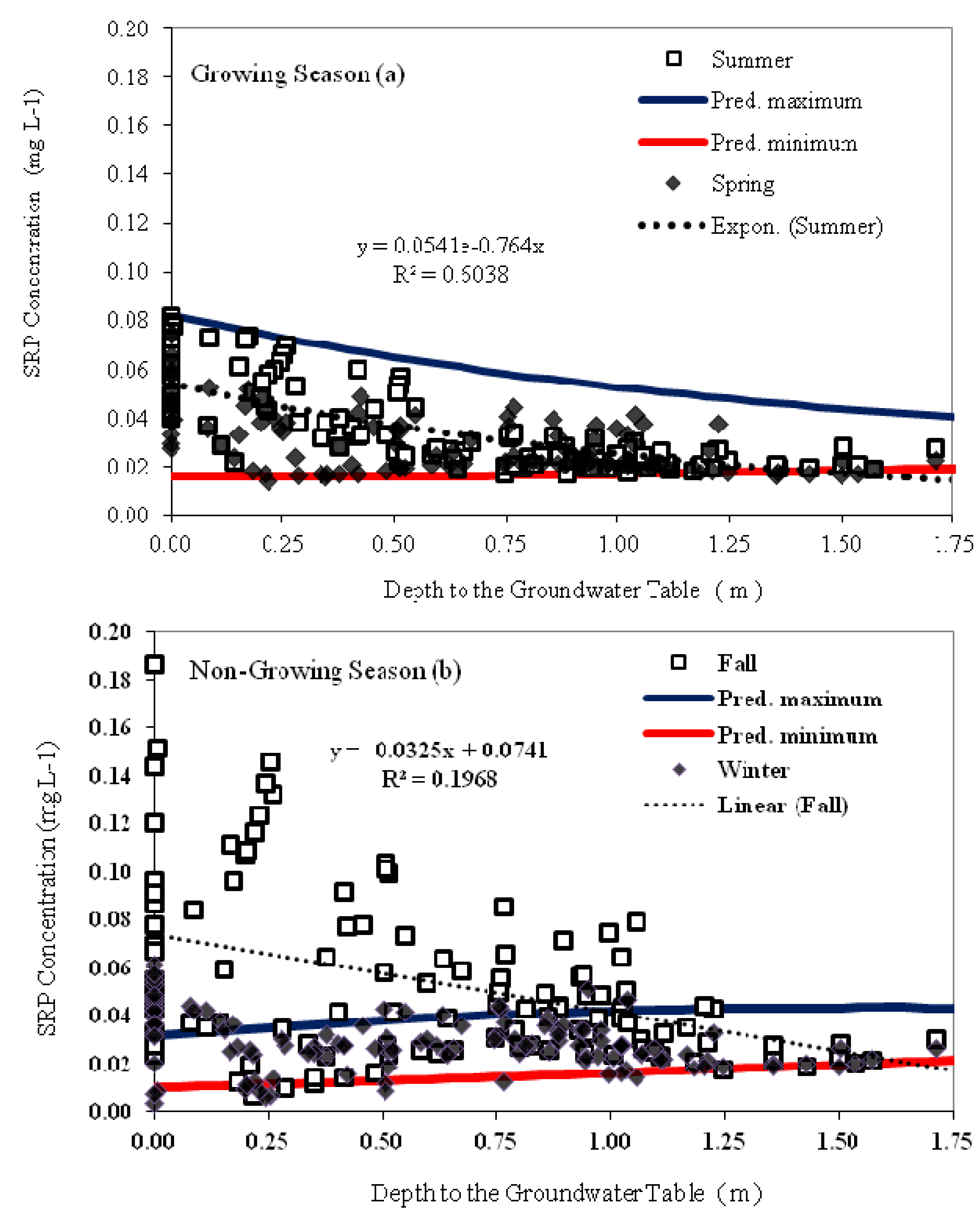
3.5. Relationship between Groundwater SRP Concentrations, Temperature and Groundwater Depth

The distance along the streamline to Creek B and the average SRP concentration for the area drained by Creek B is plotted in Figure 6 for each of the seasons of the year. Most elevated SRP concentrations occur in fall within 75 m from the Creek B (Figure 6b). SRP concentrations during winter are all below 0.06 mg L−1 and there is no distinct trend with distance to stream unlike for the fall (Figure 6a). SRP summer and spring concentrations (Figure 6a) are less than the concentrations during fall and greater than the concentrations in winter (Figure 6b). The minimum concentrations are decreasing with distance to stream for the growing season. Note that at distances at more than 150 m there are much high values that deviated from the main regression line. This is probably caused by the decreasing effect of preferential flow as the groundwater becomes deeper and hence it is likely there are fewer connected macropores to that depth, meaning that only for large rainfall events water and P will penetrate to that depth. Similarly, such a trend does not exist for distances close to the creek, especially in fall, when the high concentrations are likely caused by preferential transport of SRP rich water from the manure spread at the surface. These findings are similar to that of Carlyle and Hill [53] in an agricultural region of southern Ontario, Canada where concentrations closer to the stream were greater than sampling points located at 100–140 m from the stream (<0.025 mg L−1).
Figure 6. Predicted groundwater SRP concentration for each 10-m cell size draining into Creek B based on the predicted groundwater SRP concentration map for (a) growing- and (b) non-growing seasons and corresponding flow distance to Creek B obtained from the MODFLOW model.
Water 05 00540 g006
Since manure has been spread over these fields for more than 100 years there is a strong indication from the literature that SRP concentration are greater when saturated conditions occur in the P rich labile pool layer [5,7], one can expect that some of the variation in SRP concentration with distance to stream is caused by the depth of the groundwater. We re-plotted the data of Figure 5 with respect to water table depth (Figure 7). Groundwater depth was obtained from MODFLOW for each 10 m grid. Especially for the summer when leaching is rare, we see a general increase in P values with decrease in water table depth. (A fitted exponential curve to data is shown in Figure 7a and shows an upward trend with an R2 of 0.60). During the fall there was a similar trend of increasing concentrations with decreasing water table depth, but due to the large scatter, the fit was poorer. However, this increasing trend does not exist in general for the winter except when the water table is within 25 cm of the ground surface. Similar to spring, only when the water table is within 25 cm of the soil surface, concentration increases (trend lines are not shown). Thus, the different behavior of the concentrations with depth greater than 25 cm for fall and summer compared with spring and winter cannot be explained by more P in the profile near the surface as suggested by the authors in Florida [28,29] because the response would be independent of time. Therefore, other factors must be affecting the P concentration. We propose that these are the soil temperature and preferential transport of P after early fall manure applications when plant uptake has diminished, and these factors are discussed in the following paragraph.
Figure 7. Observed SRP concentrations in groundwater plotted against groundwater depth. (a) SRP concentration for the spring and summer (growing season). Solid lines are predicted outer bounds of concentrations. The black solid line is the maximum concentration during the warmest time of year. The red solid line is the minimum concentrations expected to occur when the temperatures in the soil are the coolest at the beginning of spring when the growing season starts; (b) SRP concentration for the fall and winter (non-growing season). Solid lines are predicted outer bounds of the concentration. The black solid line is the maximum concentration during the beginning of fall when the temperatures are the warmest during the non-growing season. The red solid line is the minimum concentrations expected to occur when the temperatures are lowest in January.
Water 05 00540 g007
In order to predict the impact of temperature, we first determine the soil temperatures at the water table with Equation (2). Since thermal diffusivity is almost independent of moisture content [8], we use DT = 0.04 m2 day−1 (Table 3). Once we have determined the soil temperature, the Arrhenius relationship (Equation (1)) is employed to estimate the maximum and minimum concentration during the growing and non-growing seasons. The maximum concentration is calculated by using the warmest days during each of the periods. This is the middle of the summer for growing period (20 July) and the beginning of fall (21 September) for the non-growing periods. The minimum concentrations are estimated by using the coldest day during each of the periods, 20 January for the non-growing season and 21 March for the growing season (Figure 7). For the X factor in Equation (2) that determines how much the reaction increases for a 10 °C rise in temperature, the same value X = 2.5 is used as per Hively et al. ([49]; and Table 3). The reference concentration, Cref = 0.03 mg L−1, is the same as the average concentration in baseflow omitting the few high concentrations that were influenced by surface runoff. Tref is equal to the annual average year temperature (Table 3).
Table 3. Parameter values used for predicting soil temperature and SRP boundaries [Equations (1) and (2)].
ParameterParameter DescriptionParameter ValueUnit
CrefReference concentration0.03mg L−1
XFactor change for a 10 °C change in temperature2.5-
TaAnnual average air temperature 7°C
ΔTAnnual amplitude12°C
tϕTime lag from 1 January120d
DT Thermal diffusivity0.04m2/day
Figure 7 shows that during three of the four seasons (winter, spring and summer), the observed points fell well within the outer bounds predicted with the Arrhenius equation for the coldest and warmest days indicating that soil temperature is an important factor in changing the concentration from one season to the next. This is similar to the seasonal change in SRP that other studies have found [31,32,54,55]. It shows that in addition to effects of seasonal variation in the dominant hydrologic pathway and in-stream control via high rates of net nutrient uptake [56], an increase in temperature directly or indirectly can promote the SRP release in the groundwater, most likely by stimulating chemical and microbiological processes [34,36,57,58].
Only during the fall, the maximum predicted phosphorus concentration with the Arrhenius equation does not reflect the observed concentrations (Figure 7b). There are many points above the line but none below it. These elevated concentrations are not observed during other periods of the year. It has been shown that high P concentrations soon after manure application can be attributed to preferential flow through macropores with almost no bounding of P to the column [59]. We therefore expect that some of the high concentrations found in this study are caused by preferential flow from the fall applied manure, after crop nutrient uptake ceases. In summer when evaporation exceeds the precipitation, there is usually very little leaching. The application of manure in winter and spring occurs when the soil temperatures are at their lowest; the result of cold temperatures and temperature damping at depth. During the fall period the soil temperature is still relatively warm so the labile pool of P, especially the organic fraction of ligand exchange and complexation, is still quite active and decomposing. Spreading manure wastewater at this time has the effect of decreasing the zero-sorption P equilibrium concentration and reducing the amount of P that can be stored in the labile pool [60]. In addition, the mineralization and subsequent accumulation of P in the summer may add to the leaching of P in the fall. The coarse loamy (low clay content) soil texture in this alluvial valley bottom soil also does not exhibit much potential for precipitation or adsorption of the released P to iron/aluminum oxides, so, upon wetting and reduction of the organic pool in the fall, the released P is rapidly mobilized to the shallow groundwater.

3.6. Best Management Practices

Nutrient management can affect the groundwater in two ways. Concentrations in the top 25 cm were usually increased independent of the time of the year (Figure 7). When groundwater approaches the soil surface in the near-stream areas, the elevated concentration of P at the soil surface has a direct effect on the P concentration in the water’s zone. In such cases a reduction in the surface concentration P by applying less manure in these areas will reduce P concentrations in the near stream areas. This practice has been effective in the upland areas of the Catskills Mountains Best management practices (BMPs) that prevented the spreading of manure in near stream areas and high P fields have been shown to be an effective way to manage P in runoff [18,61,62]. A second effect of management on groundwater is the time of spreading. We did not see any high concentration of P in groundwater during spring because manure applied throughout the winter probably increased the soil organic matter somewhat, which subsequently increases the P sorption maximum. Although the largest P losses from manure occur shortly after spreading in liquid manure handling systems [59], this farm applied more solid manure that contains higher amounts of organic material. In fall when manure was applied we noted high concentration in groundwater especially after large storms (such as in [44]) when preferential flow with the SRP from the manure was likely the cause of these high concentrations. After high concentrations occur, the concentrations at the next sampling date decreased [12] because of interactions with the soil matrix. By applying manure in areas where the groundwater is deep, P can be absorbed by a greater soil mass, avoiding preferential transport of P and decreasing the concentration of the matrix. This in turn results in decreasing the equilibrium concentration of groundwater SRP.

4. Conclusions

In this study, groundwater and stream flow were monitored over a two year period to quantify the impact of ecological and physical drivers on SRP groundwater concentrations in a valley dairy farm in the Catskill Mountains of New York State. MODFLOW was used to simulate the steady state groundwater streamlines. Kriging was employed to estimate spatial SRP patterns in groundwater. SRP concentrations were greater during the warm periods when the chemical and microbial processes were enhanced. SRP concentrations predicted with the Arrhenius equation (using groundwater temperatures as input) bounded the observed SRP concentration, with the exception of the fall when preferential flow was likely responsible for the increased P concentrations. In addition, where groundwater was within the root zone, SRP concentrations were elevated. Hence, management practices that include land application of manure at times when soils are relatively dry and on fields where groundwater recharge is minimal, i.e., fields with a deep groundwater table, will minimize baseflow SRP concentrations.

Acknowledgements

The authors would like thank the farm family for allowing us on their farm. Specifically we are grateful for their interest in the project and assistance with the research. The project was part of the USDA CEAP program (USDA-SCREES grants 00-51-130-9777 and 2007-51130-03992) and was carried out in cooperation with theWatershed Agricultural Council, Delaware County of Watershed Affairs, New York City Department of Environmental Protection, and New York State Department of Environmental Conservation.

References

  1. Puckett, L.J. Identifying the major sources of nutrient water pollution. Environ. Sci. Technol. 1995, 29, 408A–414A. [Google Scholar]
  2. Sharpley, A.N.; McDowell, R.W.; Weld, J.L.; Kleinman, P.J.A. Assessing site vulnerability to phosphorus loss in an agricultural watershed. J. Environ. Qual. 2001, 30, 2026–2036. [Google Scholar] [CrossRef]
  3. Domagalski, J.L.; Ator, S.; Coupe, R.; McCarthy, K.; Lampe, D.; Sandstrom, M.; Baker, N. Comparative study of transport processes of nitrogen, phosphorus, and herbicides to streams in five agricultural basins, USA. J. Environ. Qual. 2008, 37, 1158–1169. [Google Scholar] [CrossRef]
  4. Dingman, S.L. Physical Hydrology, 2nd ed; Prentice Hall: Upper Saddle River, NJ, USA, 2002. [Google Scholar]
  5. Gburek, W.J.; Sharpley, A.N. Hydrologic controls on phosphorus loss from upland agricultural watersheds. J. Environ. Qual. 1998, 27, 267–277. [Google Scholar] [CrossRef]
  6. Schilling, K.E.; Jacobson, P. Groundwater nutrient concentrations near an incised midwestern stream: Effects of floodplain lithology and land management. Biogeochemistry 2008, 87, 199–216. [Google Scholar] [CrossRef]
  7. Sharpley, A.N.; Chapra, S.; Wedepohl, R.; Sims, J.T.; Daniel, T.C.; Reddy, K. Managing agricultural phosphorus for protection of surface waters: Issues and options. J. Environ. Qual. 1994, 23, 437–451. [Google Scholar]
  8. Steenhuis, T.S.; Bodnar, M.; Geohring, L.D.; Aburime, S.-A.; Wallach, R. A simple model for predicting solute concentration in agricultural tile lines shortly after application. Hydrol. Earth Syst. Sci. Discuss. 1997, 1, 823–833. [Google Scholar] [CrossRef]
  9. United States Environmental Protection Agency (USEPA), National Water Quality Inventory: Report to Congress; USEPA: Washington, DC, USA, 2009.
  10. Laboski, C.A.M.; Lamb, J.A. Impact of manure application on soil phosphorus sorption characteristics and subsequent water quality implications. Soil Sci. 2004, 169, 440–448. [Google Scholar]
  11. New York State Department of Environmental Conservation (NYSDEC), New York State Fact Sheet: Ambient Water Quality Value for Protection of Recreational Uses; Bureau of Technical Services and Research: Albany, NY, USA, 1993.
  12. Flores-López, F.; Easton, Z.M. A multivariate analysis of covariance to determine the effects of near-stream best management practices on nitrogen and phosphorus concentrations on a dairy farm in the New York Conservation Effects Assessment Project watershed. J. Soil. Water Conserv. 2010, 65, 438–449. [Google Scholar] [CrossRef]
  13. Kleinman, P.J.A.; Allen, A.L.; Needelman, B.A.; Sharpley, A.N.; Vadas, P.A.; Saporito, L.S.; Folmar, G.J.; Bryant, R.B. Dynamics of phosphorus transfers from heavily manured coastal plain soils to drainage ditches. J. Soil. Water Conserv. 2007, 62, 225–235. [Google Scholar]
  14. Murray, T.P. Evaluating Level-Lip Spreader Vegetative Filter Strips in Removing Phosphorus from Milkhouse Waste in New York City’s Water Supply Watersheds. Master Thesis, Cornell University, Ithaca, NY, USA, 2001. [Google Scholar]
  15. Kim, Y.J.; Geohring, L.D.; Jeon, J.H.; Collick, A.S.; Giri, S.K.; Steenhuis, T.S. Evaluation of the effectiveness of vegetative filter strips for phosphorus removal with the use of a tracer. J. Soil Water Conserv. 2006, 61, 293–302. [Google Scholar]
  16. Bishop, P.L.; Hively, W.D.; Stedinger, J.R.; Rafferty, M.R.; Lojpersberger, J.L.; Bloomfield, J.A. Multivariate analysis of paired watershed data to evaluate agricultural best management practice effects on stream water phosphorus. J. Environ. Qual. 2005, 34, 1087–1101. [Google Scholar] [CrossRef]
  17. Brannan, K.M.; Mostaghimi, J.A.; Mcclellan, P.W.; Inamdar, S. Animal waste BMP impacts on sediment and nutrient losses in runoff from the Owl Run watershed. Trans. ASAE 2000, 43, 1155–1166. [Google Scholar]
  18. Easton, Z.M.; Walter, M.T.; Steenhuis, T.S. Combined monitoring and modeling indicate the most effective agricultural best management practices. J. Environ. Qual. 2008, 37, 1798–1809. [Google Scholar] [CrossRef]
  19. Gitau, M.W.; Veith, T.L.; Gburek, W.J. Farm-level optimization of BMP placement for cost-effective pollution reduction. Trans. ASAE 2004, 47, 1923–1931. [Google Scholar]
  20. Inamdar, S.P.; Mostaghimi, S.; Mcclellan, P.W.; Brannan, K.M. BMP impacts on sediment and nutrient yields from an agricultural watershed in the coastal plain region. Trans. ASAE 2001, 44, 1191–1200. [Google Scholar]
  21. Lee, K.-H.; Isenhart, T.M.; Schultz, R.C.; Mickelson, S.K. Multispecies riparian buffers trap sediment and nutrients during rainfall simulations. J. Environ. Qual. 2000, 29, 1200–1205. [Google Scholar]
  22. Heathwaite, A.; Dils, R. Characterising phosphorus loss in surface and subsurface hydrological pathways. Sci. Total Environ. 2000, 251–252, 523–538. [Google Scholar]
  23. Brodie, J.E.; Mitchell, A.W. Nutrients in Australian tropical rivers: Changes with agricultural development and implications for receiving environments. Mar. Freshw. Res. 2005, 56, 279–302. [Google Scholar] [CrossRef]
  24. Rasiah, V.; Moody, P.W.; Armour, J.D. Soluble phosphate in fluctuating groundwater under cropping in the north-eastern wet tropics of Australia. Soil Res. 2011, 49, 329–342. [Google Scholar] [CrossRef]
  25. Stedinger, J.R.; Vogel, R.M.; Foufoula-Georgiou, E. Frequency analysis of extreme events. In Handbook of Hydrology; Maidment, D.R., Ed.; McGraw-Hill, Inc.: New York, NY, USA, 1993; Chapter 18; pp. 18.11–18.66. [Google Scholar]
  26. Spalding, R.F.; Exner, M.E. Occurrence of nitrate in groundwater: A review. J. Environ. Qual. 1993, 22, 392–402. [Google Scholar] [CrossRef]
  27. Wayland, K.G.; Hyndman, D.W.; Boutt, D.; Pijanowski, B.C.; Long, D.T. Modelling the impact of historical land uses on surface-water quality using groundwater flow and solute-transport models. Lakes Reserv. 2002, 7, 189–199. [Google Scholar]
  28. Obour, A.K.; Silveira, M.L.; Vendramini, J.M.B.; Sollenberger, L.E.; O’Connor, G.A. Fluctuating water table effect on phosphorus release and availability from a Florida Spodosol. Nutr. Cycl. Agroecosyst. 2011, 91, 207–217. [Google Scholar] [CrossRef]
  29. Martin, H.W.; Ivanoff, D.B.; Graetz, D.A.; Reddy, K.R. Water table effects on histosol drainage water carbon, nitrogen, and phosphorus. J. Environ. Qual. 1997, 26, 1062–1071. [Google Scholar]
  30. Scott, C.A.; Walter, M.F.; Nagle, G.N.; Walter, M.T.; Sierra, N.V.; Brooks, E.S. Residual phosphorus in runoff from successional forest on abandoned agricultural land: 1. Biogeochemical and hydrological processes. Biogeochemistry 2001, 55, 293–310. [Google Scholar] [CrossRef]
  31. Duan, S.; Kaushal, S.S.; Groffman, P.M.; Band, L.E.; Belt, K.T. Phosphorus export across an urban to rural gradient in the Chesapeake Bay watershed. J. Geophys Res. Biogeosci. 2012, 117, G01025. [Google Scholar] [CrossRef]
  32. Lutz, B.D.; Mulholland, P.J.; Bernhardt, E.S. Long-term data reveal patterns and controls on stream water chemistry in a forested stream: Walker Branch, Tennessee. Ecol. Monographs 2012, 82, 367–387. [Google Scholar] [CrossRef]
  33. Hively, W.D.; Bryant, R.B.; Fahey, T.J. Phosphorus concentrations in overland flow from diverse locations on a New York dairy farm. J. Environ. Qual. 2005, 34, 1224–1233. [Google Scholar] [CrossRef]
  34. Bailey, J.E.; Ollis, D.F. Biochemical Engineering Fundamentals; McGraw-Hill Inc.: New York, NY, USA, 1986. [Google Scholar]
  35. Frossard, E.; Condron, L.M.; Oberson, A.; Sinaj, S.; Fardeau, J.C. Process governing phosphorus availability in temperate soils. J. Environ. Qual. 2000, 34, 15–23. [Google Scholar]
  36. Hansen, N.C.; Daniel, T.C.; Sharpley, A.N.; Lemunyon, J.L. The fate and transport of phosphorus in agricultural systems. J. Soil Water Conserv. 2002, 57, 408–417. [Google Scholar]
  37. Blecken, G.T.; Zinger, Y.; Deletic, A.; Fletcher, T.D.; Hedstrom, A.; Viklander, M. Laboratory study on stormwater biofiltration Nutrient and sediment removal in cold temperatures. J. Hydrol. 2010, 394, 507–514. [Google Scholar] [CrossRef]
  38. Bunnell, F.L.; Tait, D.E.N.; Flanagan, P.W.; van Cleve, K. Microbial respiration and substrate weight loss. I. A general model of the influences of abiotic variables. Soil Biol. Biochem. 1977, 9, 33–40. [Google Scholar] [CrossRef]
  39. Clesceri, N.L.; Curran, S.J.; Sedlak, R.L. Nutrient loads to Wisconsin lakes: Part I. Nitrogen and phosphorus export coefficients. Water Resour. Bull. 1986, 22, 983–990. [Google Scholar] [CrossRef]
  40. Hanrahan, G.; Gledhill, M.; House, W.A.; Worsfold, P.J. Phosphorus loading in the Frome catchment, UK: Seasonal refinement of the coefficient modeling approach. J. Environ. Qual. 2001, 30, 1738–1746. [Google Scholar] [CrossRef]
  41. Johnsson, H.; Bergstrom, L.; Jansson, P.E. Simulated nitrogen dynamics and losses in a layered agricultural soil. Agric. Ecosyst. Environ. 1987, 18, 333–356. [Google Scholar] [CrossRef]
  42. Sharpley, A.N.; Kleinman, P.J.A.; McDowell, R.W.; Gitau, M.; Bryant, R.B. Modeling phosphorus transport in agricultural watersheds: Processes and possibilities. J. Soil Water Conserv. 2002, 57, 425–439. [Google Scholar]
  43. Kuo, W.L. Spatial and Temporal Analysis of Soil Water and Nitrogen Distribution in Undulating Landscapes Using a GIS-Based Model; Cornell University Press: Ithaca, NY, USA, 1998. [Google Scholar]
  44. Flores-Lopez, F.; Easton, Z.M.; Geohring, L.D.; Steenhuis, T.S. Factors affecting dissolved phosphorus and nitrate concentrations in ground and surface water for a valley dairy farm in the northeastern United States. Water Environ. Res. 2011, 83, 116–127. [Google Scholar] [CrossRef]
  45. Soren, J. The Ground-Water Resources of Delaware County, New York; U.S. Bulletin GW-50; New York State Water Resources Commission: Albany, NY, USA, 1963.
  46. National Climatic Data Center (NCDC), Climatological Data Annual Summary-New York; NCDC: Asheville, NC, USA, 2000.
  47. Method 4500-P G (Ortho-P) and Method 4500-Ph (Total P). In Apha/Awwa/Wef.: Standard Methods for the Examination of Water and Wastewater; American Public Health Association: Washington, DC, USA, 1999.
  48. Environmental Systems Research Institute (ESRI), ArcGIS; ESRI: Redlands, CA, USA, 2007.
  49. Hively, W.D.; Gérard-Marchant, P.; Steenhuis, T.S. Distributed hydrological modeling of total dissolved phosphorus transport in an agricultural landscape, part II: Dissolved phosphorus transport. Hydrol. Earth Sys. Sci. Discuss. 2006, 10, 263–276. [Google Scholar] [CrossRef]
  50. De Vries, D.A. Thermal properties of soils. In Physics of Plant Environment; van Wijk, W., Ed.; North Holland Pub. Co.: Amsterdam, NL, USA, 1963; pp. 210–235. [Google Scholar]
  51. Brutsaert, W. Evaporation into the Atmosphere; D. Reidel Publishing Co.: Boston, MA, USA, 1982. [Google Scholar]
  52. Young, E.O.; Briggs, R.D. Phosphorus concentrations in soil and subsurface water: A field study among cropland and riparian buffers. J. Environ. Qual. 2008, 37, 69–78. [Google Scholar] [CrossRef]
  53. Carlyle, G.C.; Hill, A.R. Groundwater phosphate dynamics in a river riparian zone: Effects of hydrologic flowpaths, lithology and redox chemistry. J. Hydrol. 2001, 247, 151–168. [Google Scholar] [CrossRef]
  54. McDowell, R.; Trudgill, S. Variation of phosphorus loss from a small catchment in south Devon, UK. Agric. Ecosyst. Environ. 2000, 79, 143–157. [Google Scholar] [CrossRef]
  55. Neal, C.; Reynolds, B.; Neal, M.; Hughes, S.; Wickham, H.; Hill, L.; Rowland, P.; Pugh, B. Soluble reactive phosphorus levels in rainfall, cloud water, throughfall, stemflow, soil waters, stream waters and groundwaters for the Upper River Severn area, Plynlimon, mid Wales. Sci. Total Environ. 2003, 314–316, 99–120. [Google Scholar] [CrossRef]
  56. Mulholland, P.J.; Hill, W.R. Seasonal patterns in streamwater nutrient and dissolved organic carbon concentrations: Separating catchment flow path and in-stream effects. Water Resour. Res. 1997, 33, 1297–1306. [Google Scholar] [CrossRef]
  57. Correll, D.L.; Jordan, T.E.; Weller, D.E. Effects of precipitation and air temperature on phosphorus fluxes from rhode river watersheds. J. Environ. Qual. 1999, 28, 144–154. [Google Scholar] [CrossRef]
  58. Duan, S.; Amon, R.; Bianchi, T.S.; Santschi, P.H. Temperature control on soluble reactive phosphorus in the lower Mississippi river? Estuaries Coasts 2011, 34, 78–89. [Google Scholar] [CrossRef]
  59. Geohring, L.D.; McHugh, O.V.; Walter, M.T.; Steenhuis, T.S.; Akhtar, M.S.; Walter, M.F. Phosphorus transport into subsurface drains by macropores after manure applications: Implications for best manure management practices. Soil Sci. J. 2001, 166, 896–909. [Google Scholar]
  60. Zhang, W.; Faulkner, J.W.; Giri, S.K.; Geohring, L.D.; Steenhuis, T.S. Effect of soil reduction on phosphorus sorption of an organic-rich silt loam. Soil Sci. Soc. Am. J. 2010, 74, 240–249. [Google Scholar]
  61. Dittrich, T.M.; Geohring, L.D.; Walter, M.T.; Steenhuis, T.S. Revisiting Buffer Strip Design Standards for Removing Dissolved and Particulate Phosphorus. In Proceedings of Total Maximum Daily Load (TMDL) Environmental Regulations–II Conference, Albuquerque, NM, USA, 8–12 November 2003; 2003; pp. 527–534. [Google Scholar]
  62. James, E.; Kleinman, P.; Veith, T.; Stedman, R.; Sharpley, A. Phosphorus contributions from pastured dairy cattle to streams of the Cannonsville Watershed, New York. J. Soil. Water Conserv. 2007, 62, 40–47. [Google Scholar]

