Article

Evaluation of Hyperspectral Multi-Band Indices to Estimate Chlorophyll-A Concentration Using Field Spectral Measurements and Satellite Data in Dianshan Lake, China

1
Department of Environmental Science and Engineering, Fudan University, Shanghai 200433, China
2
The State Key Laboratory of Remote Sensing Science, Jointly Sponsored by the Institute of Remote Sensing Applications of Chinese Academy of Sciences and Beijing Normal University, Institute of Remote Sensing Applications, Chinese Academy of Sciences, Beijing 100101, China
3
Department of Geography & Environmental Studies, California State University, San Bernardino, CA 92407, USA
4
Coastal Ecosystems Research Station of Yangtze River Estuary, Institute of Biodiversity Science, Fudan University, Shanghai 200433, China
5
Department of Geography, University of California, Santa Barbara, CA 93106, USA
6
Shanghai Environmental Monitoring Center, Shanghai 200030, China
*
Author to whom correspondence should be addressed.
Water 2013, 5(2), 525-539; https://doi.org/10.3390/w5020525
Submission received: 19 February 2013 / Revised: 25 March 2013 / Accepted: 2 April 2013 / Published: 29 April 2013

Abstract

:
Chlorophyll-a (Chl-a) concentration is considered as a key indicator of the eutrophic status of inland water bodies. Various algorithms have been developed for estimating Chl-a in order to improve the accuracy of predictive models. The objective of this study is to assess the potential of hyperspectral multi-band indices to estimate the Chl-a concentration in Dianshan Lake, which is the largest lake in Shanghai, an international metropolis of China. Based on field spectral measurements and in-situ Chl-a concentration collected on 7–8 September 2010, hyperspectral multi-band indices were calibrated to estimate the Chl-a concentration with optimal wavelengths selected by model tuning. A three-band index accounts for 87.36% (R2 = 0.8736) of the Chl-a variation. A four-band index, which adds a wavelength in the near infrared (NIR) region, results in a higher R2 (0.8997) by removing the absorption and backscattering effects of suspended solids. To test the applicability of the proposed indices for routinely monitoring of Chl-a in inland lakes, simulated Hyperion and real HJ-1A satellite data were selected to estimate the Chl-a concentration. The results show that the explanatory powers of these satellite hyperspectral multi-band indices are relatively high with R2 = 0.8559, 0.8945, 0.7969, and 0.8241 for simulated Hyperion and real HJ-1A satellite data, respectively. All of the results provide strong evidence that hyperspectral multi-band indices are promising and applicable to estimate Chl-a in eutrophic inland lakes.

1. Introduction

Lake water quality is important for the development of aquaculture, sightseeing, and transportation, etc. With the rapid development of economy, industrialization and human activities in China, pollution and eutrophication problems of lake water resources are becoming increasingly severe. Since the end of the last century, cyanobacteria algal blooms have occurred in many lakes of China, which has been worsening in recent years [1]. The cyanobacteria blooms have caused the death of a large number of aquatic animals and led to stench in lake water. Chlorophyll-a (Chl-a) concentration is considered as a key indicator of the eutrophic status of inland water bodies [2]. As Chl-a exists in all algae groups in marine and freshwater systems, Chl-a concentration is always deemed as a proxy of cyanobacteria algal biomass in waters [3]. Therefore, it is practicable to map the amount of cyanobacteria and to predict cyanobacteria algae blooms through the index of Chl-a [4]. Chl-a concentration is also an important index for detecting the degree of pollution in inland water bodies.
Compared to traditional Chl-a monitoring methods through extensive field sampling, which are time-consuming and difficult to perform for large-scope regional and global studies, remote sensing provides near real-time, large-scale and spatially continuous information [5]. However, accurate estimates of Chl-a concentration with remote sensing data is challenging in inland Case II waters [6,7,8]. In order to overcome the optical complexities of Case II waters, the red and near-infra-red (NIR) spectral regions have been used as the effects of suspended particulate matter (SPM) and colored dissolved organic matter (CDOM) decrease at longer wavelengths [9].
Various algorithms have been developed for estimating Chl-a concentration in eutrophic and turbid Case II waters based on the spectral characteristics in the red and NIR regions [9,10,11]. Thiemann and Kaufman used the 705 nm to 678 nm reflectance ratio to assess Chl-a concentration in Mecklenburg Lake [12]. Jiao et al. [13] extended the method by using the 719 nm to 667 nm reflectance ratio according to the inherent spectral properties of Taihu Lake. To account for the variability in scattering among samples, Zimba et al. [14] proved that a three-band index originally developed for estimating chlorophyll content in terrestrial vegetation [15,16] could be applied to the estimation of Chl-a in waters with high accuracy.
However, the assumptions for the three-band semi-analytical algorithm may be complicated in highly turbid waters. For example, Tzortziou et al. [17] showed that the absorption by particulate matter in the 700–730 nm regions could not be neglected in Chesapeake Bay. Tassan and Ferrari [18] found that the aquatic particle absorption significantly varied with the type of suspended particles. Recently, an enhanced three-band index, i.e., a four-band index [19], which adds a reflectance band in the NIR, was proposed to estimate Chl-a concentration in turbid waters. With the additional fourth band, the four-band index can remove the absorption and backscattering by suspended solids over the NIR region, and minimize the absorption by pure water.
In order to apply multi-band indices routinely, Gons et al. [20] and Moses et al. [2,21] went further to implement the three-band index using MERIS and MODIS images, to successfully estimate Chl-a concentrations in inland lakes and coastal waters. However, the advent of hyperspectral sensor technology has allowed improving the models with subtle reflection features. Instead of the broadband of multispectral data, hyperspectral satellite data with a spectral resolution of 5–10 nm can capture various physical and biological characteristics of inland waters [22,23]. Therefore, the physically-based abilities of hyperspectral remote sensing are highly suitable for Chl-a estimation and have the possibility to assess all optical water parameters in Case II waters [24].
For the hyperspectral satellite data that can be applied to multi-band indices, Hyperion and HJ-1A are two potential choices for Chl-a estimation in Case II waters [4,25]. In particular, the HJ-1A satellite, which was launched in September 2008, is equipped with a hyper-spectral imager (HSI) that can capture images of the Earth surface with 115 bands over the spectral range from 450 to 950 nm. The superiority also includes a high spectral resolution of 5 nm and a spatial resolution of 100 m. In addition, the revisit time is only four days, which is more appropriate for timely Chl-a concentration monitoring.
The objectives of the study include: (1) to identify the characteristics of field spectral reflectance and to establish hyperspectral multi-band indices for Chl-a estimation in Dianshan Lake; (2) to evaluate the accuracy and sensitivity of the proposed three-band and four-band indices; (3) to assess the potential of hyperspectral satellite data to estimate Chl-a concentration in eutrophic inland lakes.

2. Study Area and Datasets
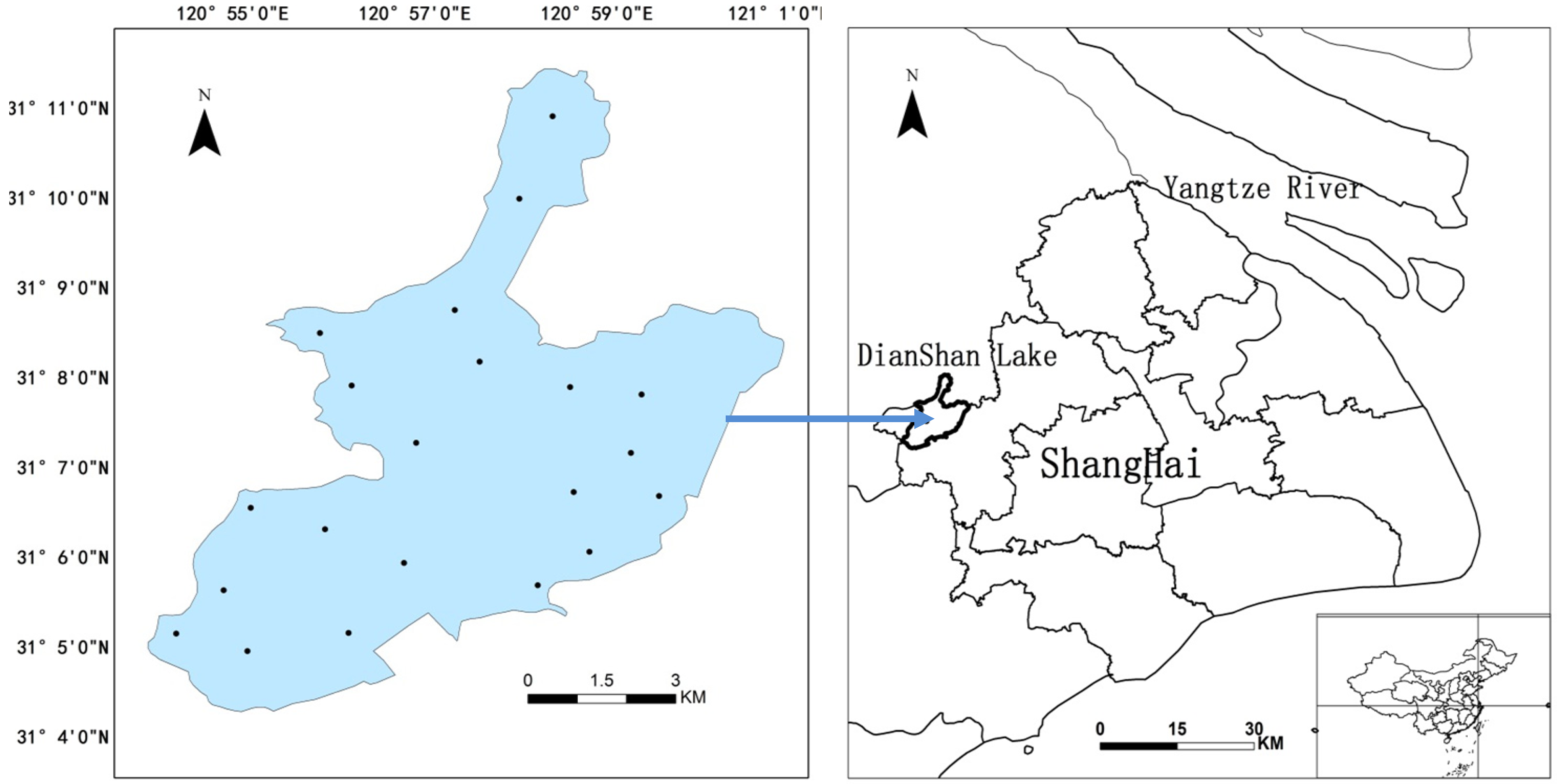
2.1. Study Area

In this paper, a typical inland freshwater lake—Dianshan Lake—was selected as the study area. Dianshan Lake is the largest lake in Shanghai, an international metropolis in Eastern China, located between 30°12' N and 31°04' N, and 120°54' E and 121°01' E (Figure 1). The lake has an average surface area of 62 km2, and a mean water depth of 2.11 m. The water flow rate is very slow, typically only 0.03 m/s, and the water exchange period is nearly 24 days in the low-water season. An annual average water surface temperature is about 18.8 °C. The lake is of considerable interest because it provides more than 60% of the water supply for local residents [1] and is mainly used for drinking water, navigation, irrigation, and flood control. As a result, the water yield and quality of the lake are important to people’s daily life and to the social and economic development of Shanghai city.

2.2. Field Spectral Measurements Data

Field spectral measurements and in-situ Chl-a data were acquired on 7–8 September 2010. The spectral measurements were taken from a boat using an Analytical Spectral Devices (ASD) FieldSpec Spectroradiometer, which measures reflected radiance between 350 nm and 1075 nm at an increment of 1.5 nm in 512 bands. The raw data were transformed by the instrument software, so the output measurements had a sampling interval of 1 nm. During the measurements, the instrument was hand-held with a field view of 25° and positioned approximately 1 m above the water surface. Intercalibration of the radiometers was completed by measuring the upwelling radiance of a white spectralon panel. The “above water method” was used to measure the water surface spectra [26,27], and the reflectance measurements followed the Ocean Optical protocols (Revision 3) by NASA (2002). The water surface reflectance spectra were measured at least ten times at each sample station. A mean value after median filtering was taken as the final result. Considering the synchronization between the in-situ data and the satellite overpass, water samples and reflectance measurements were collected between 10:00 am and 12:00 pm at local time. Due to the low water transparency (the average transparency < 0.5 m) in the lake, the reflectance from the bottom of the lake was negligible.
Figure 1. Location of Dianshan Lake and the distribution of sample sites.
Water 05 00525 g001

2.3. In-situ Chl-a Data

Water samples were collected from a shallow water depth (50 cm below surface) at 30 sample sites in different regions of Lake Dianshan. In the laboratory, the water samples were filtered through 0.45 µm filters, left overnight at 4 °C in the dark, and then extracted with 95% acetone. Subsequently, the clarified liquid was quantified using the UV-2501 spectrophotometer [28], and the Chl-a concentrations were calculated according to Scientific Committee on Oceanic Research-United Nations Educational, Scientific and Cultural Organization equations [29,30]. Water filters were dried at 105 °C for 4 h and then weighed to obtain total suspended solids (TSS). For all the 30 water samples, the Chl-a concentrations ranged from 5.53 mg/m3 to 100.3 mg/m3, with an average of 27.74 mg/m3. The concentrations of TSS were between 20.1 mg/m3 and 72 mg/m3, with an average of 37.27 mg/m3. The water sampling was performed during the summer when the wind speed was relatively low. Therefore, the disturbance effect due to the presence of wind could be neglected.

3. Analyses

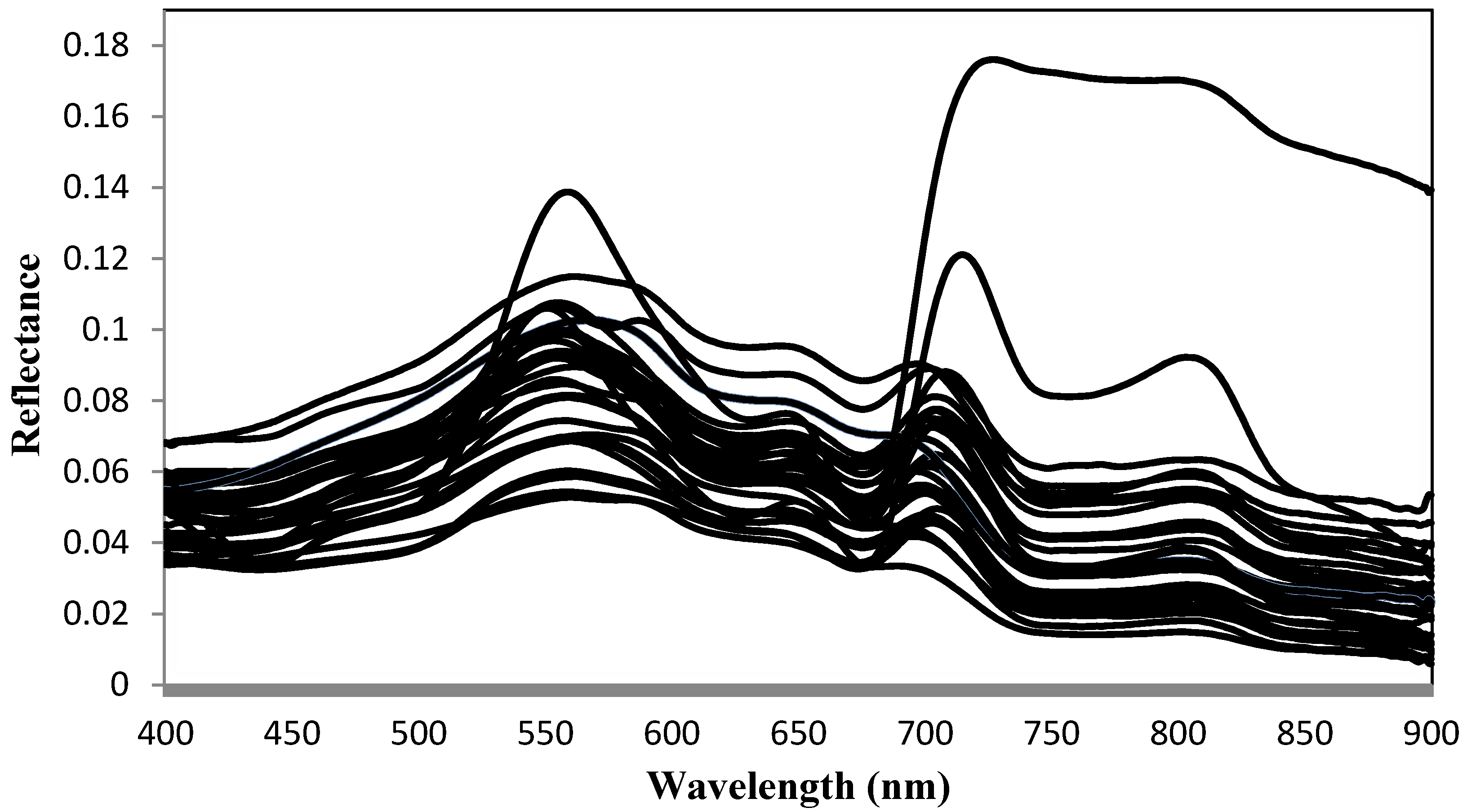
3.1. Spectral Reflectance Properties

Specific spectral analysis is needed in order to choose the sensitive wavelengths and to optimize the multi-band combination. Figure 2 shows the spectral reflectance of Dianshan Lake. The reflectance was highly variable in the visible and NIR spectral regions. Yet, the shape and magnitude of the reflectance spectra were similar to those of typical productive inland water bodies [31]. Reflectance was relatively low in the blue range (400–495 nm) due to the total absorption of water constituents, but was much higher in the green range (495–570 nm). The varied presence of cyanobacteria caused a correspondingly slight reflectance trough around 620 nm and a unique reflectance peak around 650 nm as the water was dominated by cyanobacteria algae [18,32]. The significant spectral characteristic was the reflectance peak around 700 nm, of which the peak shifted from 690 to 715 nm with the increase of Chl-a concentration [24,33]. In the NIR region, the reflectance trough around 730 nm was formed by the strong absorption of pure water.
Figure 2. Field spectral reflectance in Dianshan Lake.
Water 05 00525 g002

3.2. Multi-Band Indices Tuning

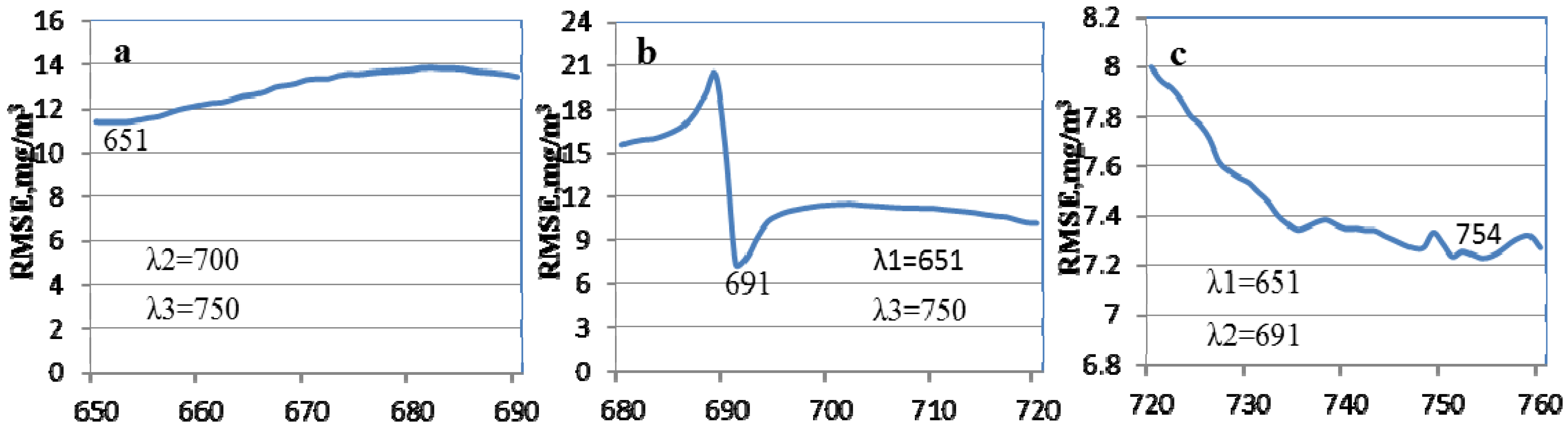
3.2.1. Three-Band Index

The three-band index, as a conceptual model developed for Chl-a estimation, has been proven robust in turbid waters [33]. The three-band index can be shown as Equation (1).
Water 05 00525 i001
λ1 is a wavelength where the Chl-a absorption has the greatest effect on remote sensing reflectance, and the absorption by CDOM and non-pigmented particles has less effect on the total backscattering, thus, λ1 should be within the red band range; λ2 is a wavelength with little absorption by Chl-a, so the fluorescence peak around 700 nm meets this requirement; the selection criteria for λ3 are that the total absorption is much larger than the backscattering, and the reflectance is mainly affected by the absorption of pure water [7,13]. As a result, the spectral ranges of the three bands should be restricted to 650–690 nm, 690–720 nm, and 720–800 nm for λ1, λ2, and λ3, respectively.
The optimal wavelengths were selected based on the minimum root mean square root (RMSE) error for Chl-a, when two wavelengths were held constant, the third wavelength was allowed to vary until the minimum RMSE error was reached. To find the optimal λ1, initial λ2 and λ3 were fixed at 700 nm and 750 nm. As λ1 was tuned from 650 nm to 690 nm, the RMSE of [Rrs−11) −Rrs−1 (700)] × Rrs (750) versus Chl-a was calculated. As a result, the optimum wavelength for λ1 occurred at 651 nm (Figure 3a). To determine the optimal position for λ2, λ1 and λ3 were fixed at 651 nm and 750 nm, while λ2 was tuned from 680 nm to 720 nm, the RMSE of index [Rrs−1 (651) −Rrs−1 (λ2)] × Rrs (750) versus Chl-a was computed for each λ2. The result shows that the minimum RMSE existed at 691 nm (Figure 3b). Similarly, the optimal value of λ3 was determined by setting λ1 = 651 nm and λ2 = 691 nm, and the minimum RMSE occurred at 754 nm (Figure 3c). We carried out the tuning process repeatedly to assess whether the optimal locations shifted to other wavelengths. Finally, the three wavelengths were selected at 651 nm, 691 nm, and 754 nm, respectively.
Figure 3. RMSE of Chl-a estimation from three-band indices versus measured Chl-a at different wavelengths. (a) Water 05 00525 i002 letting vary λ1, (b) Water 05 00525 i003 
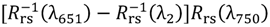
letting vary λ2 varying, (c) Water 05 00525 i004 letting vary λ3.
Water 05 00525 g003

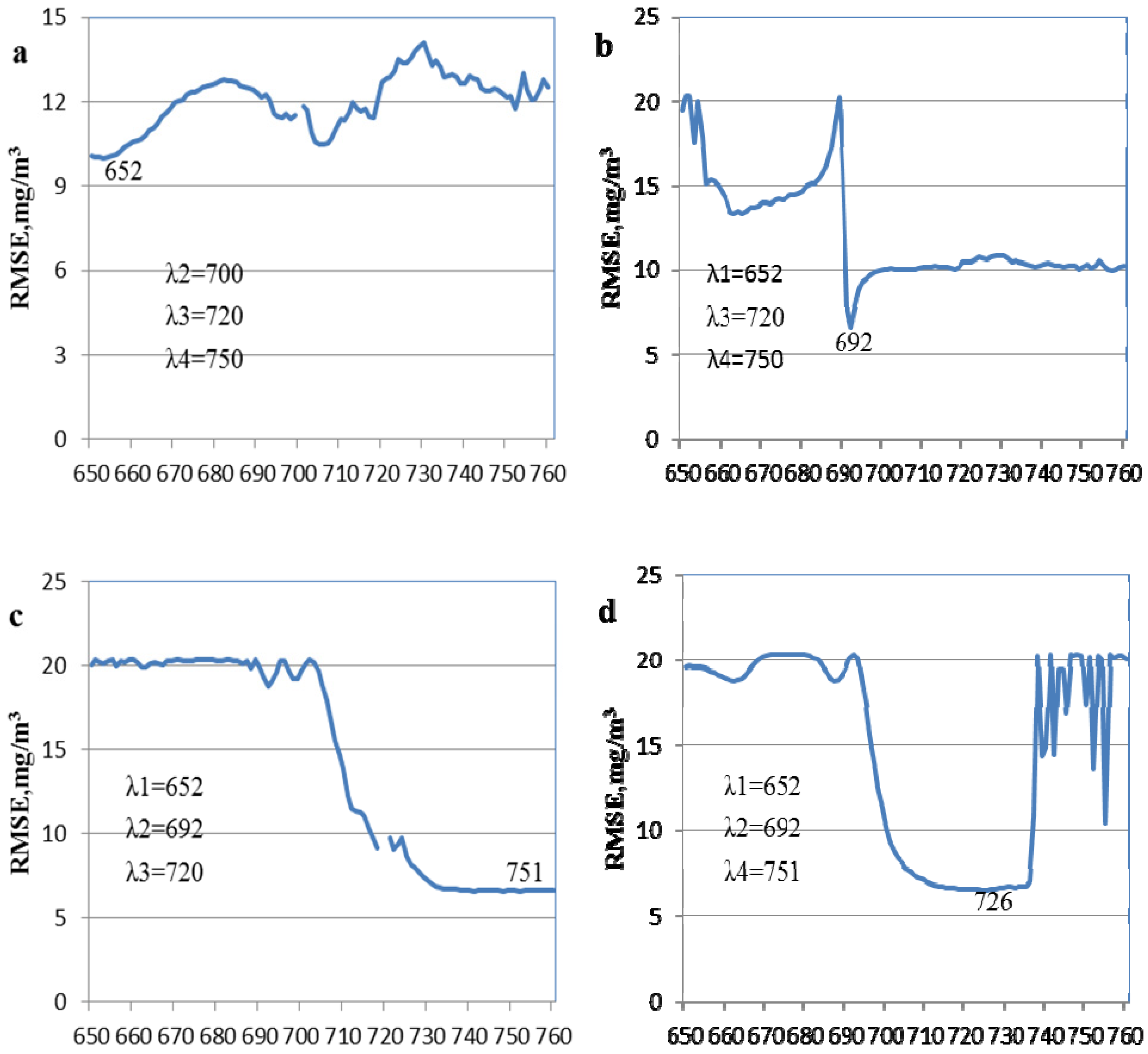
3.2.2. Four-Band Index

The four-band index was developed to improve the three-band index by replacing Water 05 00525 i005 with Water 05 00525 i006, which could subtract the effect of suspended solids and minimize the absorption by pure water as well as backscattering in NIR region [18]. The four-band index is shown as Equation (2).
Water 05 00525 i007
The optimal positions of the four wavelengths were also determined by band tuning using the same method as in previous section. To find the optimal wavelengths for the four-band index, λ1, λ2, λ3, and λ4 were all tuned in the range of 650–760 nm. We initially fixed λ2, λ3, and λ4 at 700 nm, 720 nm, and 750 nm, respectively. The minimum RMSE occurred at 652 nm by tuning λ1 from 650 nm to 760 nm, (Figure 4a). Thus, 652 nm was selected for λ1. To determine the optimal position of λ2, λ1, λ3, and λ4 were fixed at 652 nm, 720 nm, and 750 nm, respectively. The tuning result shows that the optimal position of λ2 was located at 692 nm (Figure 4b). When λ1 = 652 nm, λ2 = 692 nm and λ3 = 720 nm, RMSE became minimal at 751 nm for λ4 (Figure 4c). Similarly, when λ1 = 652 nm, λ3 = 720 nm, and λ4 = 750 nm, the optimum location of λ3 occurred at 726 nm (Figure 6d). After tuning again to examine the selected wavelengths, the final selections for λ1, λ2, λ4, and λ3 were 652 nm, 692 nm, 751 nm, and 726 nm, respectively.
Figure 4. RMSE of Chl-a estimation from four-band indices versus measured Chl-a for optimal wavelength selection. (a) Water 05 00525 i008; (b) Water 05 00525 i009; (c) Water 05 00525 i010; (d) Water 05 00525 i011.
Water 05 00525 g004

4. Results

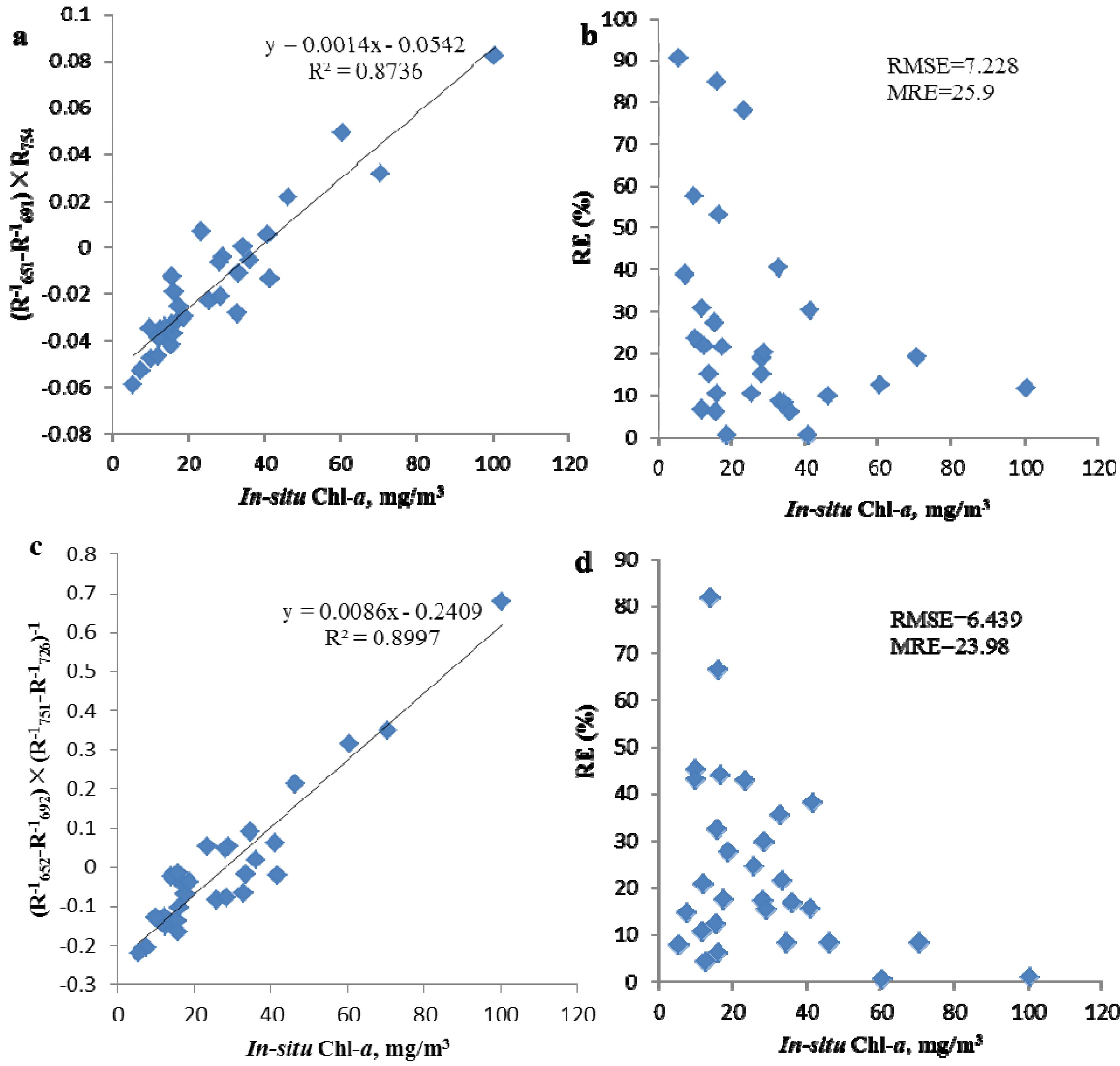
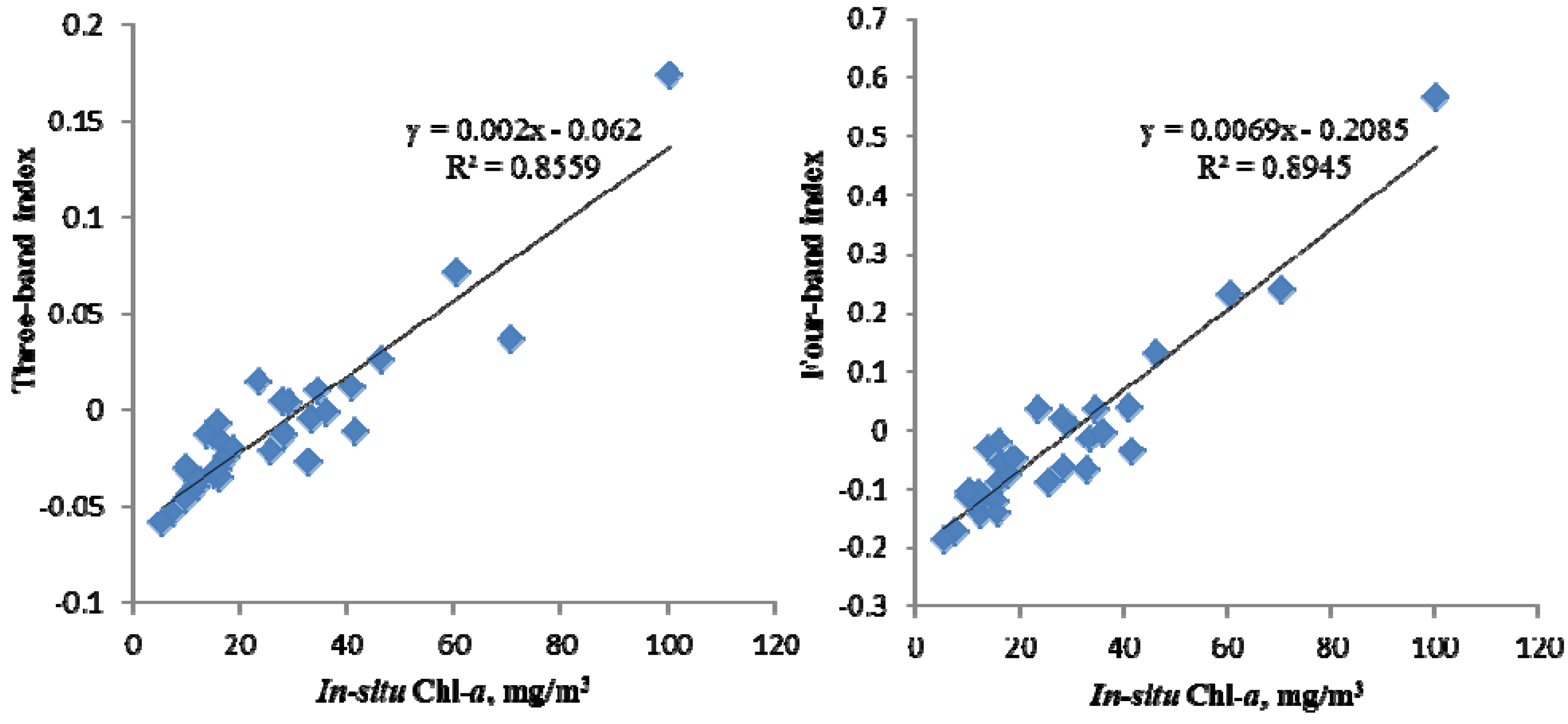
4.1. Estimation of Chl-a Concentration with Field Spectral Multi-Band Indices

The relationships between the index values and Chl-a concentrations were determined using linear regression. Although in most cases a non-linear model produced a better fit than a linear model, the latter can maintain a stable performance across different water bodies, and thus can better describe the practicability and universality of the relationships. Based on the wavelengths determined above, the linear relationships between the multi-band indices and Chl-a concentration were calculated as follows [Equation (3) for three-band index and Equation (4) for four-band index].
Water 05 00525 i012
Water 05 00525 i013
Both the three-band and the four-band indices had close relationships with the Chl-a concentration. The three-band index was positively related to the Chl-a concentration with R2 = 0.8736 (Figure 5a). The four-band index, which minimized the backscattering by suspended solids and absorption by pure water, showed a stronger relationship with the Chl-a concentration with R2 = 0.8997 (Figure 5c). The RMSE also decreased from 7.228 mg/m3 for the three-band index regression model to 6.439 mg/m3 for the four-band index regression model, which was far below the average Chl-a concentration of 27.74 mg/m3. All the above indicates that the four-band index has a superior performance to the three-band index.
Figure 5. Linear regression of field spectral multi-band indices versus in-situ Chl-a concentrations. (a) Linear regression for three-band index; (b) relative error (RE) of the linear regression for three-band index; (c) Linear regression for four-band index; (d) RE of the linear regression for four-band index.
Water 05 00525 g005
The relationship between relative error (RE) and in-situ Chl-a concentration was also evaluated to compare the ability of the two indices in estimating Chl-a. Both Figure 6b,d illustrate that RE decreases with the increase of the Chl-a concentration. The mean relative error (MRE) of the four-band index was lower than that of the three-band index, decreasing from 25.9 mg/m3 for the three-band index (Figure 5b) and to 23.98 mg/m3 for the four-band index (Figure 5d). It is noted that the RE decrease is more evident in the sample sites with higher Chl-a concentration. That is, the four-band index in particular was appropriate for the estimation of higher Chl-a concentration.

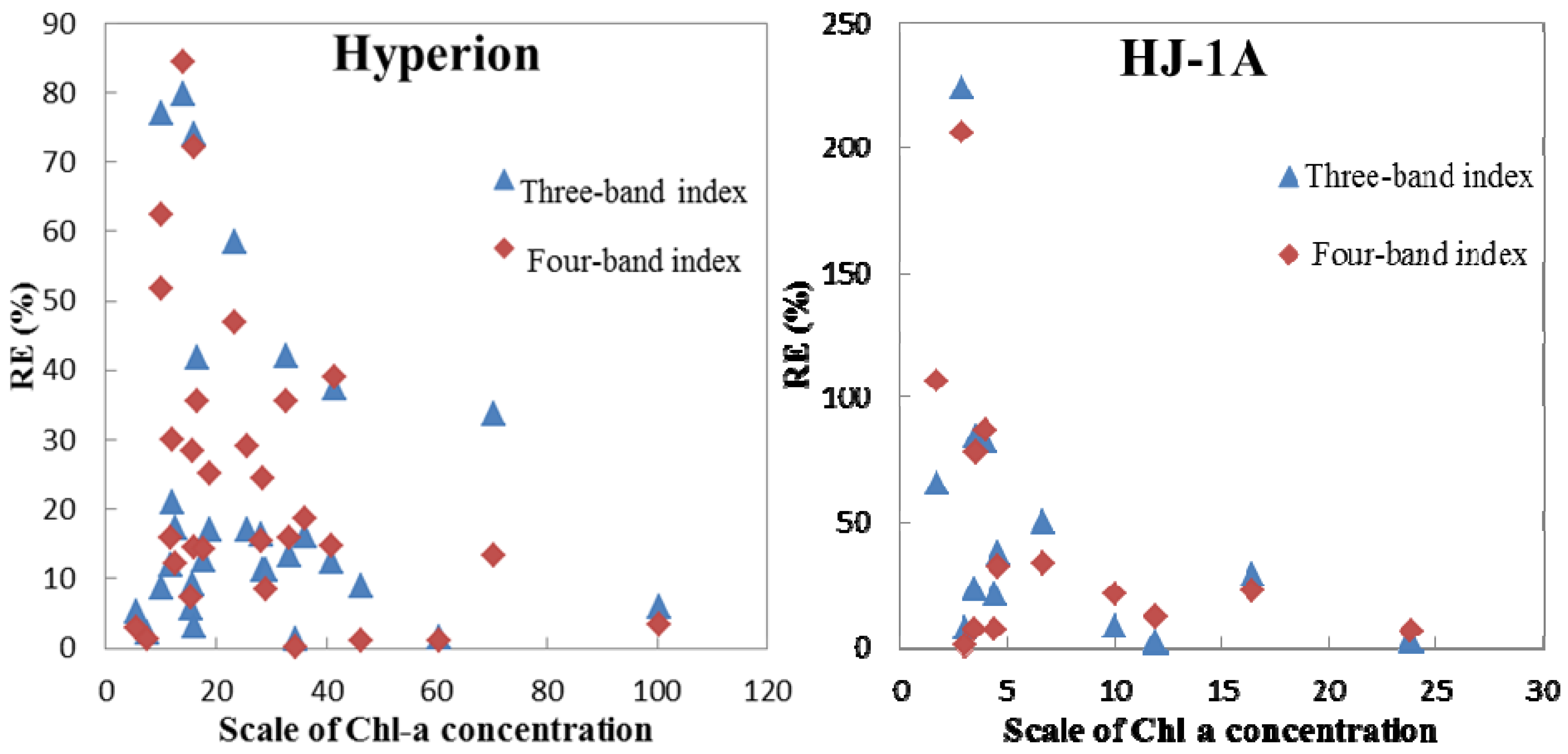
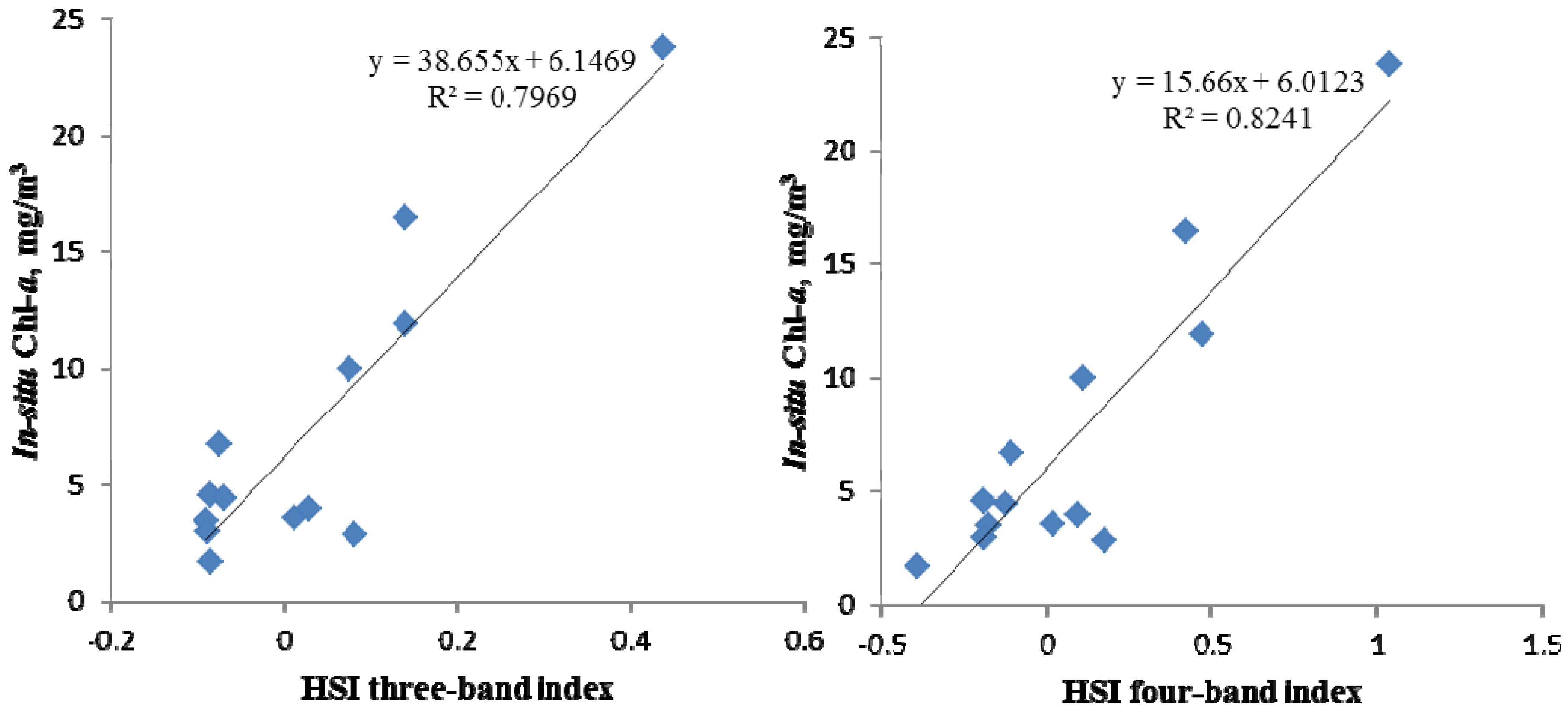
4.2. Estimation of Chl-a Concentration with Satellite Hyperspectral Multi-Band Indices

Hyperion is a popular hyperspectral satellite data, which can meet the band requirements of multi-band indices [30,34], and HJ-1A is a new hyperspectral satellite launched by China [25]. Therefore, the performance and robustness of the three-band and four-band indices were evaluated using simulated Hyperion data and real HJ-1A hyperspectral satellite data.
To be consistent, the simulated Hyperion bands used in the indices were obtained from equivalent wavelengths in the field spectral measurements. Since the bandwidth of Hyperion data is about 10 nm [35], the measured reflectances were averaged to the corresponding spectral bands of Hyperion to simulate the reflectance of Hyperion satellite hyperspectral bands. The optimal bands for the three-band index were B30 (647–656 nm), B34 (687–696 nm) and B40 (748–757 nm), and the optimal bands for the four-band index were B30 (647–656 nm), B34 (687–696 nm), B37 (718–727 nm) and B40 (748–757 nm), respectively.
In the simulated Hyperion band reflectance, the indices accounted for 85.59% and 89.45% of the total variance in Chl-a concentration for three-band index and four-band index, respectively (Figure 6). The RMSEs were 7.718 mg/m3 in the three-band regression model and 6.603 mg/m3 in the four-band regression model, which were both far below the average Chl-a concentration. Like the results in Section 4.1, the model accuracy of the four-band index was also higher than that of the three-band index. The relatively high accuracies demonstrated the potential of Hyperion multi-band indices in estimating Chl-a concentration.
Figure 6. Accuracy assessment of the two indices with simulated bands of Hyperion. (a) Three-band index; (b) Four-band index.
Water 05 00525 g006
In order to overcome the deficiency of simulated data in real application, a HJ-1A HSI image acquired on 23 August 2010 and in situ Chl-a concentration data synchronously obtained were used to further test the applicability of the multi-band indices. Preprocessing is required on the raw satellite hyperspectral data to obtain the remote sensing reflectance. We used the method of by-band 6S-atmospheric-correction [36]. In this procedure, the atmospheric model was Mid-Latitude summer and the aerosol model was the continental aerosol type. Together with the altitude value and wavelengths setting of the image sensor, remote sensing reflectance at all wavelengths was retrieved and used for Chl-a estimation. The band setting of the HSI sensor is shown in Table 1.
Table 1. Bands setting of HJ-1A HSI.
Band numberSpectral range (nm)Center wavelength (nm)Band numberSpectral range (nm)Center wavelength (nm)
66650–654.18652.0979709–713.99711.495
67654.18–658.43656.30580713.99–719.04716.515
68658.43–662.72660.57581719.04–724.17721.605
69662.72–667.08664.982724.17–729.37726.77
70667.08–671.49669.28583729.37–734.65732.01
71671.49–675.96673.72584734.65–740.01737.33
72675.96–680.49678.22585740.01–745.44742.725
73680.49–685.08682.78586745.44–750.95748.195
74685.08–689.74687.4187750.95–756.55753.75
75689.74–694.45692.09588756.55–762.23759.39
76694.45–699.24696.84589762.23–767.99765.11
77699.24–704.08701.6690767.99–773.85770.92
78704.08–709706.5491773.85–779.79776.82
For the satellite HJ-1A hyperspectral multi-band indices, the optimal bands were selected for the HJ-1A HSI data using the same approach as described in Section 3.2.1. The tuning results show that the optimal bands for the three-band index are B75 (689.74–694.45 nm), B78 (704.08–709.00 nm), and B88 (756.55–762.23 nm), and the optimal bands for the four-band index are B75 (689.74–694.45 nm), B78 (704.08–709.00 nm), B81 (719.04–724.17 nm), and B86 (745.44–750.95 nm), respectively. The calibrated HJ-1A multi-band index regression models are shown in the following equations [Equation (5) for three-band index, and Equation (6) for four-band index] as well as in Figure 8.
Water 05 00525 i014
Water 05 00525 i015
The three-band index, based on the bands of B75, B78, and B88, explained 79.69% of the total Chl-a variance and could be used to estimate Chl-a concentration with RMSE less than 2.82 mg/m3 (Figure 7a). The four-band index based on the bands of B75, B78, B81, and B86 accounted for 82.41% of the total Chl-a variance and was able to estimate the Chl-a concentration with a RMSE of less than 2.623 mg/m3 (Figure 7b). Although the R2 for the HJ-1A data models were a little lower than those for the simulated Hyperion data models, they were still high enough for practical Chl-a concentration estimation. The lower accuracies may have resulted from the process of atmosphere correction or the settings of the sensor’s channel.
Figure 7. Linear regression and accuracy assessment of the two indices with hyperspectral reflectance of HJ-1A. (a) Three-band index regression; (b) Four-band index regression.
Water 05 00525 g007
Figure 8 shows the relationships between the in-situ Chl-a concentration and the REs for the two types of satellite data. For the simulated Hyperion bands, the MRE of the four-band index model was lower than that of the three-band index model, especially in the sample sites with higher Chl-a concentration (Figure 8a). For the estimation of Chl-a with HSI data, the MRE of the four-band index regression model was also lower than that of the three-band index model (Figure 8b), which echoed the higher R2 discussed above (0.8241 for four-band index regression vs. 0.7969 for three-band index regression). The largest RE occurred at the sample site with low Chl-a concentration, which was probably caused by the effects of clouds and can be considered as an abnormal value.
Figure 8. The relationships between RE and Chl-a concentration. (a) Hyperion data; (b) HJ-1A data.
Water 05 00525 g008

5. Discussion and Conclusions

With the development of remote sensing technology, timely monitoring of Chl-a concentration for inland lake waters using hyperspectral satellite data can be achieved with a relatively high accuracy and will be a trend for future research [30]. The narrow and contiguous bands of hyperspectral data can reflect the important characteristics of every kind of water quality parameters. Therefore, we can use hyperspectral data to find the optimal bands for multi-band indices and can improve the model accuracy.
The selected wavelengths for the multi-band indices in this paper differed slightly from previous studies [2,37]. Most other studies focused on the first wavelength selection at around 670 nm, but due to the higher Chl-a concentration in this study, we determined λ1 at around 650 nm, which is a critical location to the first band in multi-band indices for high Chl-a concentration [38,39]. The second wavelength we selected was just beyond 690 nm, different from the selection of reflectance peak at 700 nm in other studies [40,41]. The reason may be that after the first wavelength was determined, the small distance between the first two bands could minimize the effects of CDOM and Tripton.
Comparing the selected bands of the two indices, we found that the optimum wavelengths of the three-band index were 651 nm, 691 nm, and 754 nm, while those of the four-band index were 652 nm, 692 nm, 726 nm, and 751 nm. In the four-band index, except for the 726 nm, the other three selected bands were almost the same as those in the three-band index. The wavelength selection results illustrated that the four-band index was indeed an improvement of the three-band index [19], and in most cases, there was no need to tune the model again to find the already-determined three bands for the four-band index.
For the multi-band indices based on the field spectral measurements, the MRE of Chl-a concentrations estimated were only 25.90% for the three-band index and 23.98% for the four-band index, respectively. The RMSE was 7.228 mg/m3 in the three-band index model and decreased to 6.439 mg/m3 in the four-band index regression, both far below the average Chl-a concentration. The results proved that the two indices were appropriate for the estimation of Chl-a concentration in Dianshan Lake. For turbid water bodies with high Chl-a concentration, the four-band index generated a more accurate result than the three-band index.
The semi-analytical approach used in the manuscript is also a theoretically based model and provides a practical choice for future estimation of Chl-a concentration. When applying the multi-band indices to real satellite data, due to the absence of spectral response characteristics of the low Chl-a concentration, the estimate accuracy in some sample sites may not be high enough, but the estimation results are still within the allowable error interval (with a confidence level of 95%). Moreover, the estimate accuracy of satellite hyperspectral multi-band indices in this paper was not lower than in physical-based bio-optical models [17,24].
The field spectral-based indices were the premise and foundation of the multi-band indices calculated with the satellite data. Using the simulated Hyperion data and HJ-1A hyperspectral satellite data, we also estimated the Chl-a concentration with relatively high accuracies. The two selected types of hyperspectral satellite data, both with high spatial resolution (≤100 m) and high spectral resolution (5–10 nm), were appropriate for the estimation of Chl-a concentration, particularly for biologically complex water bodies such as eutrophic inland lakes. All the results demonstrated that the two multi-band indices built on satellite data could be used to effectively and efficiently estimate Chl-a concentration on a regular basis.

Acknowledgements

This work was funded partially by National Natural Science Foundation of China (No. 41001234), Specialized Research Fund for the Doctoral Program of Higher Education of China (2010007120013), Open Fund of State Key Laboratory of Remote Sensing Science (Grant No. OFSLRSS201009), Open Fund of State Key Laboratory of Ocean Circulation and Waves, Chinese Academy of Sciences (No. KLOCAW1107), and the Fundamental Research Funds for the Central Universities. The authors are grateful to all the members who participated in the fieldwork and experimental analysis. The authors also appreciate the two anonymous reviewers’ valuable comments on the manuscript.

References

  1. Cheng, X.; Li, X. Long-term changes in nutrients and phytoplankton response in Lake Dianshan, a shallow temperate lake in China. J. Freshwater Ecol. 2010, 25, 549–554. [Google Scholar] [CrossRef]
  2. Moses, W.J.; Gitelson, A.A.; Berdnikov, S. Estimation of chlorophyll-a concentration in case 2 waters using MODIS and MERIS data-successes and challenges. Environ. Res. Lett. 2009, 6, 845–849. [Google Scholar]
  3. Giardino, C.; Bresciani, M.; Pilkaitytė, R.; Bartoli, M. In situ measurements and satellite remote sensing of case 2 waters: First results from the Curonian Lagoon. Oceanologia 2010, 52, 197–210. [Google Scholar] [CrossRef]
  4. Kutser, T.; Metsamaa, L.; Strombeck, N.; Vahtmäe, E. Monitoring cyanobacteria blooms by satellite remote sensing. Estuar. Coast. Shelf Sci. 2006, 67, 303–312. [Google Scholar] [CrossRef]
  5. Kilham, N.E.; Roberts, D. Amazon River time series of surface sediment concentration from MODIS. Int. J. Remote Sens. 2011, 32, 2659–2679. [Google Scholar] [CrossRef]
  6. Darecki, M.; Stramski, D. An evaluation of MODIS and SeaWiFS bio-optical algorithms in the Baltic Sea. Remote Sens. Environ. 2004, 89, 326–350. [Google Scholar] [CrossRef]
  7. Dall’Olmo, G.; Gitelson, A.A. Effect of bio-optical parameter variability and uncertainties in reflectance measurements on the remote estimation of chlorophyll-a concentration in turbid productive waters: Modeling results. Appl. Opt. 2006, 45, 3577–3592. [Google Scholar]
  8. Lavender, S.J.; Pinkerton, M.H.; Froidefond, J.M.; Morales, J.; Aiken, J.; Moore, G.F. Sea WIFS validation in European coastal waters using optical and biogeochemical measurements. Int. J. Remote Sens. 2004, 25, 1481–1488. [Google Scholar] [CrossRef]
  9. Gitelson, A. The peak near 700 nm on radiance spectra of algae and water: Relationships of its magnitude and position with chlorophyll concentration. Int. J. Remote Sens. 1992, 17, 3367–3373. [Google Scholar] [CrossRef]
  10. Mobley, C.D.; Sundman, L.K.; Davis, C.O.; Bowles, J.H.; Downes, T.V.; Leathers, R.A.; Montes, M.J.; Bowles, J.H.; Bissett, W.P.; Kohler, D.D.R.; et al. Interpretation of hyperspectral remote-sensing imagery by spectrum matching and look-up tables. Appl. Opt. 2005, 44, 3576–3592. [Google Scholar] [CrossRef]
  11. Gitelson, A.A.; Gurlin, D.; Moses, W.; Barrow, T. A bio-optical algorithm for the remote estimation of the chlorophyll-a concentration in case 2 waters. Environ. Res. Lett. 2009, 4, 1–5. [Google Scholar]
  12. Thiemann, S.; Kaufman, H. Determination of chlorophyll content and tropic state of lakes using field spectrometer and IRS-IC satellite data in the Mecklenburg Lake Distract, Germany. Remote Sens. Environ. 2000, 73, 227–235. [Google Scholar] [CrossRef]
  13. Jiao, H.; Zha, Y.; Gao, J.; Li, Y.M.; Wei, Y.C.; Huang, J.Z. Estimation of chlorophyll-a concentration in Lake Tai, China using in-situ hyperspectral data. Int. J. Remote Sens. 2006, 27, 4267–4276. [Google Scholar] [CrossRef]
  14. Zimba, P.V.; Gitelson, A. Remote estimation of chlorophyll concentration in hyper-eutrophic aquatic systems: Model tuning and accuracy optimization. Aquaculture 2006, 256, 272–286. [Google Scholar] [CrossRef]
  15. Gitelson, A.A.; Gritz, Y.; Merzlyak, M.N. Relationships between leaf chlorophyll content and spectral reflectance and algorithms for non-destructive chlorophyll assessment in higher plant leaves. J. Plant Physiol. 2003, 160, 271–282. [Google Scholar] [CrossRef]
  16. Gitelson, A.A.; Vĭna, A.; Ciganda, V.; Rundquist, D.C.; Arkebauer, T.J. Remote estimation of canopy chlorophyll content in crops. Geophys. Res. Lett. 2005, 32, L08403. [Google Scholar]
  17. Tzortziou, M.; Herman, J.R.; Gallegos, C.L.; Neale, P.; Subramaniam, A.; Harding, L.; Ahmad, Z. Bio-optics of the Chesapeake Bay from measurements and radiative transfer closure. Estuar. Coast. Shelf Sci. 2006, 68, 348–362. [Google Scholar] [CrossRef]
  18. Tassan, S.; Ferrari, G.M. Variability of light absorption by aquatic particles in the near-infrared spectral region. Appl. Opt. 2003, 42, 4802–4810. [Google Scholar] [CrossRef]
  19. Le, C.; Li, Y.; Zha, Y.; Sun, D.; Huang, C.; Lu, H. A four-band semi-analytical model for estimating chlorophyll a in highly turbid lakes: The case of Taihu Lake, China. Remote Sens. Environ. 2009, 113, 1175–1182. [Google Scholar] [CrossRef]
  20. Gons, H.J.; Rijkeboer, M.; Ruddick, K.G. Effect of a waveband shift on chlorophyll retrieval from MERIS imagery of inland and coastal waters. J. Plankton Res. 2005, 27, 125–127. [Google Scholar]
  21. Bresciani, M.; Vascellari, M.; Giardino, C.; Matta, E. Remote sensing supports the definition of the water quality status of Lake Omodeo (Italy). Eur. J. Remote Sens. 2012, 45, 349–360. [Google Scholar]
  22. Zhou, G.; Liu, Q.; Ma, R.; Tian, G. Inversion of chlorophyll-a concentration in turbid water of Lake Taihu based on optimized multi-spectral combination. J. Lake Sci. 2008, 20, 153–159. [Google Scholar]
  23. Brando, V.E.; Dekker, A.G. Satellite hyperspectral remote sensing for estimating estuarine and coastal water quality. IEEE Trans. Geosci. Remote Sens. 2003, 41, 1378–1387. [Google Scholar] [CrossRef]
  24. Gons, H.J. Optical teledetection of chlorophyll a in turbid inland waters. Environ. Sci. Technol. 1999, 33, 1127–1132. [Google Scholar] [CrossRef]
  25. Wang, Q.; Wu, C.; Li, Q.; Li, J.S. Chinese HJ-1A/B satellites and data characteristics. Sci. China Earth Sci. 2010, 53, 51–57. [Google Scholar] [CrossRef]
  26. Mobley, C.D. Estimation of the remote-sensing reflectance from above-surface measurements. Appl. Opt. 1999, 38, 7442–7455. [Google Scholar] [CrossRef]
  27. Tang, J.W.; Tiang, G.L.; Wang, X.Y.; Wang, X.; Song, Q. The methods of water spectra measuring and analysis I: Above-water method. J. Remote Sens. 2004, 8, 37–44. [Google Scholar]
  28. Simis, S.G.H.; Peters, S.W.M.; Gons, H.J. Remote sensing of the cyanobacterial pigment phycocyanin in turbid inland water. Limnol. Oceanogr. 2005, 50, 237–245. [Google Scholar] [CrossRef]
  29. UNESCO, Determination of photosynthetic pigments in sea-water. In Monographs on Oceanographic Methodology; UNESCO: Paris, France, 1966; pp. 12–14.
  30. Chen, S.; Fang, L.; Li, H.; Chen, W.; Huang, W. Evaluation of a three-band model for estimating chlorophyll-a concentration in tidal reaches of the Pearl River Estuary, China. ISPRS J. Photogramm. Remote Sens. 2011, 66, 356–364. [Google Scholar] [CrossRef]
  31. Jupp, D.; Kirk, J.; Harris, G. Detection, identification, and mapping of cyanobacteria-using remote sensing to measure the optical quality of turbid inland waters. Aust. J. Mar. Freshwater Res. 1994, 45, 801–828. [Google Scholar] [CrossRef]
  32. Ma, R.; Dai, J.F. Investigation of chlorophyll-a and total suspended matter concentrations using Landsat ETM and field spectral measurement in Taihu Lake, China. Int. J. Remote Sens. 2005, 26, 2779–2795. [Google Scholar]
  33. Dall’Olmo, G.; Gitelson, A.A.; Rundquist, D.C.; Leavitt, B.; Barrow, T.; Holz, J.C. Assessing the potential of SeaWiFS and MODIS for estimating chlorophyll concentration in turbid productive waters using red and near-infrared bands. Remote Sens. Environ. 2005, 96, 176–187. [Google Scholar] [CrossRef]
  34. Li, L.; Li, L.; Shi, K.; Li, Z.; Song, K. A semi-analytical algorithm for remote estimation of phycocyanin in inland waters. Sci. Total Environ. 2012, 435–436, 141–150. [Google Scholar]
  35. Du, C.; Wang, S.X.; Zhou, Y.; Yan, F.L. Remote chlorophyll-a retrieval in Taihu Lake by three-band model using hyperion hyperspectral data. Environ Sci. 2009, 30, 2904–2910. [Google Scholar]
  36. Flink, P.; Lindell, T.; Oslund, C. Statistical analysis of hyperspectral data from two Swedish lakes. Sci. Total Environ. 2001, 268, 155–169. [Google Scholar] [CrossRef]
  37. Yacobi, Y.Z.; Moses, W.J.; Kaganovsky, S.; Sulimani, B.; Leavitt, B.C.; Gitelson, A.A. NIR-red reflectance-based algorithms for chlorophyll-a estimation in mesotrophic inland and coastal waters: Lake Kinneret case study. Water Res. 2011, 45, 2428–2436. [Google Scholar] [CrossRef]
  38. Schalles, J.F.; Gitelson, A.; Yacobi, Y.Z.; Kroenke, A.E. Chlorophyll estimation using whole seasonal, remotely sensed high spectral resolution data for an eutrophic lake. J. Phycol. 1998, 34, 383–390. [Google Scholar] [CrossRef]
  39. Stumpf, R.P.; Tyler, M.A. Satellite detection of bloom and pigment distributions in estuaries. Remote Sens. Environ. 1988, 24, 385–404. [Google Scholar] [CrossRef]
  40. Duan, H.; Ma, R.; Xu, J.; Zhang, Y.; Zhang, B. Comparison of different semi-empirical algorithms to estimate chlorophyll-a concentration in inland lake water. Environ. Monit. Assess. 2010, 170, 231–244. [Google Scholar] [CrossRef]
  41. Zhang, Y.; Feng, L.; Li, J.; Luo, L.; Yin, Y.; Liu, M.; Li, Y. Seasonal-spatial variation and remote sensing of phytoplankton absorption in Lake Taihu, a large eutrophic and shallow lake in China. J. Plankton Res. 2010, 32, 1023–1037. [Google Scholar] [CrossRef]

