Estimation of the Effect of Soil Texture on Nitrate-Nitrogen Content in Groundwater Using Optical Remote Sensing


Abstract
:
1. Introduction
2. Materials and Methods
2.1. Data Preparation
2.2. Data Interpolation
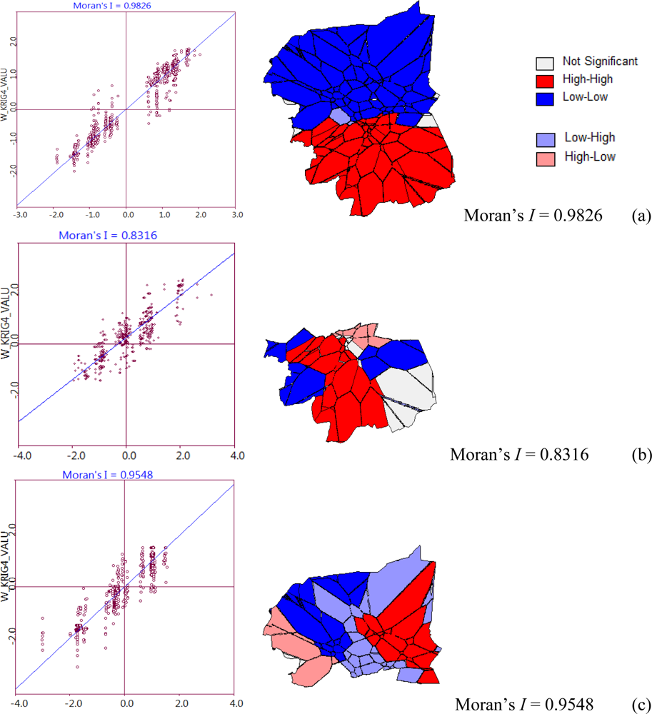
2.3. Spatial Autocorrelation Analysis
2.4. Spectral Extraction Analysis
2.5. Statistical Analysis
2.6. Software
3. Results
3.1. Data Preparation
3.1.1. LANDSAT Imagery Data
3.1.2. Soil Texture
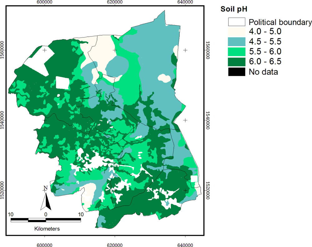
3.1.3. Soil pH
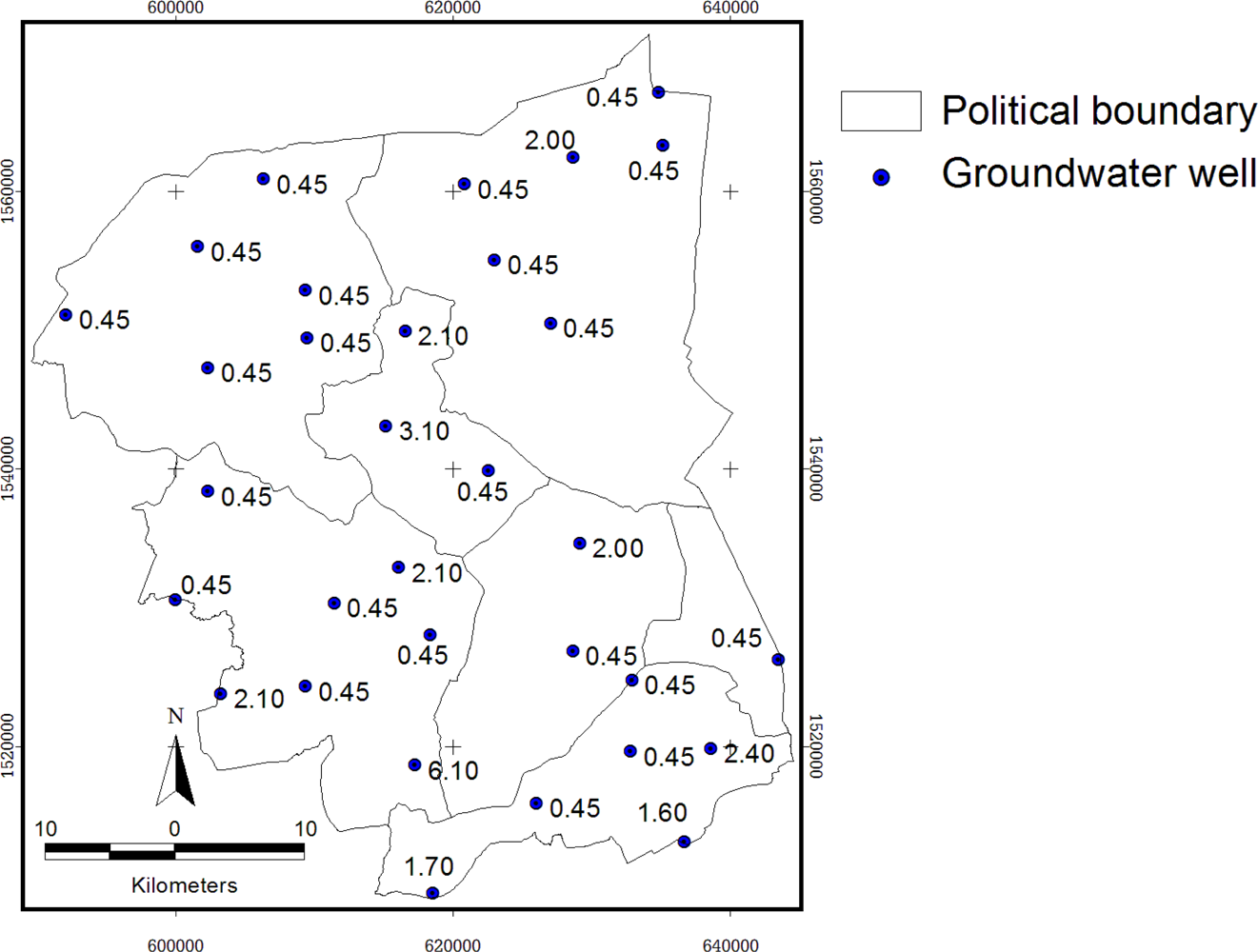
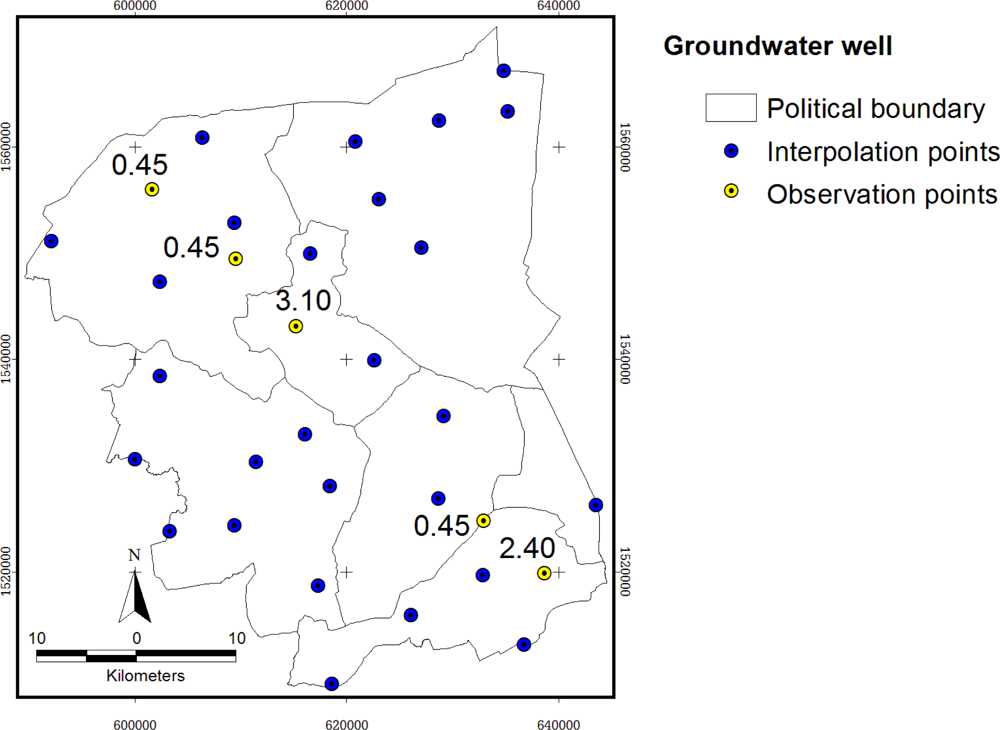
3.1.4. Groundwater Pond
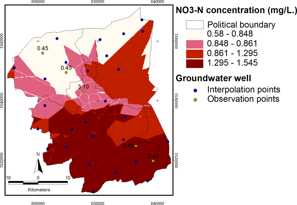
3.2. NO3−-N Interpolation
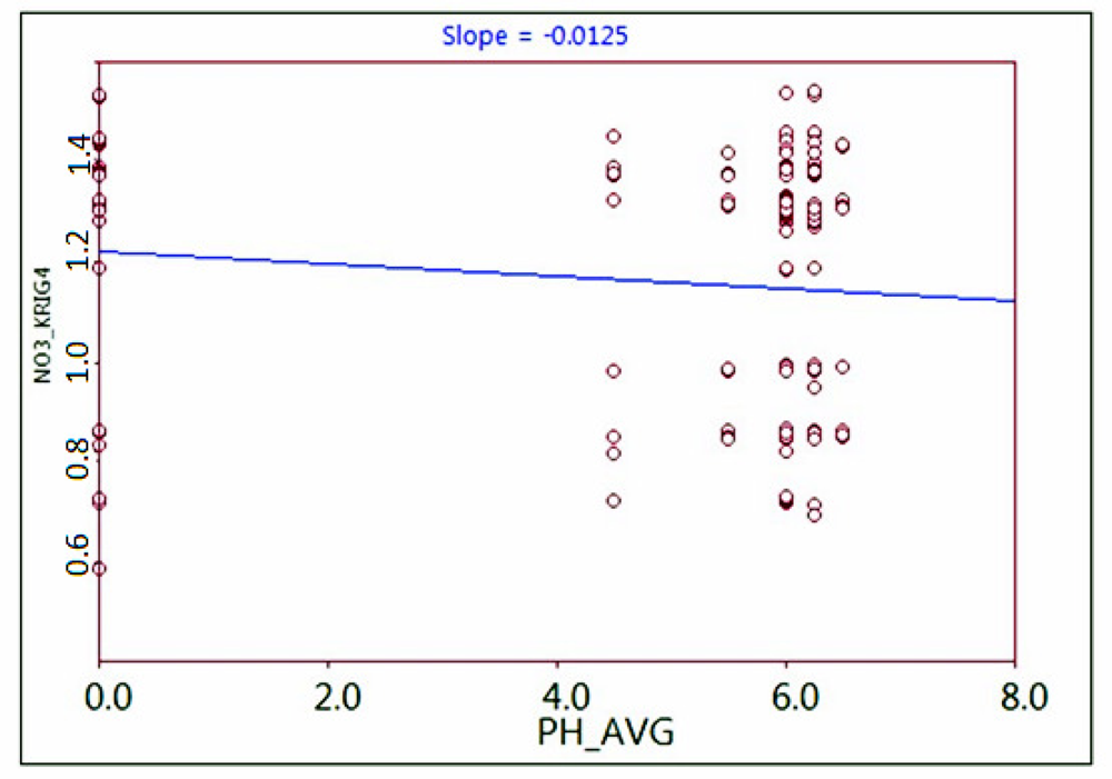
3.3. Spatial Autocorrelation Analysis
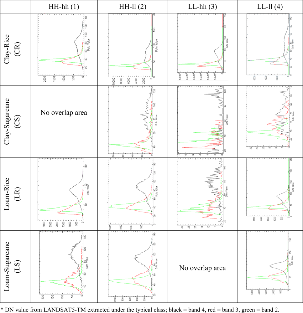
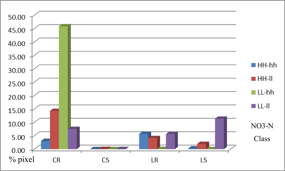
3.4. Spectral Extraction Analysis
4. Discussion
4.1. Data Preparation
4.1.1. Landuse Class
4.1.2. Soil Texture
4.1.3. Soil pH
4.1.4. Groundwater Pond
4.2. NO3−-N Interpolation
4.3. Spatial Autocorrelation Analysis
4.4. Spectral Extraction Analysis
5. Conclusions
Acknowledgments
- Conflict of InterestThe authors declare no conflict of interest.
References
- World Health Organization. Guidelines for Drinking-water Quality, 3rd ed; World Health Organization: Geneva, Switzerland, 2004; Volume 1, Recommendations. [Google Scholar]
- Tirado, R; Englande, AJ; Promakasikorn, L; Novotny, V. Technical Note 03/2008; Greenpeace Research Laboratories: Exeter, UK, 2008. [Google Scholar]
- Federal Register. National interim primary drinking water standards. Federal Register 40:59, 566588, 1975.
- Gaines, TP; Gaines, ST. Soil texture effect on nitrate leaching in soil percolates. Commun. Soil Sci. Plant Anal 1994, 25, 2561–2570. [Google Scholar]
- Alley, WM. Regional Ground Water Quality; Van Nostrand Reinhold: New York, NY, USA, 1993; p. 635. [Google Scholar]
- Reddy, AGS; Kumar, KN; Rao, SD; Rao, SS. Assessment of nitrate contamination due to groundwater pollution in north eastern part of Anantapur District, A.P. India. Environ. Monit. Assess 2009, 148, 463–476. [Google Scholar]
- Weston, D; Seelig, B. Managing Nitrogen Fertilizer to Prevent Groundwater Contamination, Extension Bulletin No. 64; North Dakota State University: Fargo, ND, USA, 1994. [Google Scholar]
- Cisse, IA; Mao, X. Nitrate: Health effect in drinking water and management for water quality. Environ. Res 2008, 2, 311–316. [Google Scholar]
- Vogt, C; Cotruvo, J. Drinking water standards: Their derivation and meaning. In Rural Groundwater Contamination; D’Itri, FM, Wolfson, LG, Eds.; Lewis Publishers: Chelsea, MI, USA, 1987; pp. 213–223. [Google Scholar]
- Rail, CD. Groundwater Contamination: Sources, Control, and Preventive Measures; Technomic Publishing Company, Inc: Lancaster, PA, USA, 1989; p. 139. [Google Scholar]
- Pathak, BK; Iida, T; Kazama, F; Jaisi, DP. Nitrogen contribution to the river basin from tropical paddy field in the central Thailand. Proceedings of 9th International River Symposium, Brisbane, Australia, 4–7 September 2006.
- Hassink, J. Effects of soil texture and grassland management on soil organic C and N and rates of C and N mineralization. Soil Biol. Biochem 1994, 26, 1221–1231. [Google Scholar]
- Brady, NC. The Nature and Properties of Soil, 8th ed; MacMillan Publishing Co. Inc: New York, NY, USA, 1974; p. 4070. [Google Scholar]
- Akram, HAH. The impact of soil texture on nitrates leaching into groundwater in the North Governorate, Gaza Strip. J. Soc. Sci 2010, 38, 1–37. [Google Scholar]
- Jackson, TJ. Remote sensing of soil moisture: implications for groundwater recharge. Hydrogeology 2002, 10, 40–51. [Google Scholar]
- Waters, P; Greenbaum, P; Smart, L; Osmaston, H. Applications of remote sensing to groundwater hydrology. Remote Sens. Rev 1990, 4, 223–264. [Google Scholar]
- Engman, ET; Gurney, RJ. Remote Sensing in Hydrology; Chapman and Hall: London, UK, 1991; p. 225. [Google Scholar]
- Meijerink, AMJ. Groundwater. In Remote Sensing in Hydrology and Water Management; Schultz, GA, Engman, ET, Eds.; Springer: Berlin, Germany, 2000; pp. 305–325. [Google Scholar]
- National Statistical Office. The 2008 Agriculture Intercensal Survey, Region: Central; National Statistical Office Publications: Bangkok, Thailand, 2008. [Google Scholar]
- Wakefield, JC; Kelsall, JE; Morris, SE. Clustering, cluster detection, and spatial variation in risk. In Spatial Epidemiology; Elliott, P, Wakefield, J, Best, N, Briggs, D, Eds.; Oxford University Press: Oxford, UK, 2000; pp. 128–152. [Google Scholar]
- Anselin, L. GeoDa 09 User’s Guide; Spatial Analysis Laboratory, University of Illinois, Urbana-Champaign: Urbana, IL, USA, 2003. [Google Scholar]
- Kriging Interpolation Extension 2.01. ESRI Inc: Redlands, CA, USA, 2010; Available online: http://arcscripts.esri.com/details.asp?dbid=10652 (accessed on 17 May 2011).
- Pick, T. Assessing the risk of ground water contamination from open lot management on Animal Feeding Operations (AFOs). Ecological Sciences—Environment Technical Note Number MT-3. Natural Resources Conservation Service: Bozeman, MT, USA, 2006; Available online: http://www.mt.nrcs.usda.gov/technical/ecs/environment/technotes/envmt3/ (accessed on 3 May 2011).
- Land Development Department (LDD). Soil Map of Nakhon Pathom 1:50,000; Ministry of Agriculture and Cooperatives: Bangkok, Thailand, 2007. [Google Scholar]
- Food and Agriculture Organization of the United Nations (FAO), Land Development Department (LDD). Soil Interpretation Hand Book for Thailand; Ministry of Agriculture and Cooperatives: Bangkok, Thailand, 1973; p. 178. [Google Scholar]
- Basin Development Plan Unit. Thai National Mekong Committee. Ministry of Natural Resources and Environment. In Sub-area Study and Analysis 5T Sub-Area; Thai National Mekong Committee: Bangkok, Thailand, 2004. [Google Scholar]
- Newman, JA; Bergelson, J; Grafen, A. Blocking factors and hypothesis tests in ecology: Is your statistics text wrong? Ecology 1997, 78, 1312–1320. [Google Scholar]
- McDonald, JH. Handbook of Biological Statistics, 2nd ed; Sparky House Publishing: Baltimore, MD, USA, 2009; pp. 127–129. [Google Scholar]
- National Statistical Office. The 2008 Agriculture Intercensal Survey, Whole Kingdom; National Statistical Office Publications: Bangkok, Thailand, 2008. [Google Scholar]


| Class | pH range | Group of soil series * | Min | Max | Average | Area (Km2) |
|---|---|---|---|---|---|---|
| 1 | 4.0–5.0 | 11, 11f | 4.0 | 5.0 | 4.5 | 125.32 |
| 2 | 5.0–5.5 | 2, 2f, 2/11 | 5.0 | 6.0 | 5.5 | 554.83 |
| 3 | 5.5–6.0 | 1, 1/2, 1f, 4, 4/38 | 5.5 | 6.5 | 6.0 | 451.94 |
| 4 | 6.0–6.5 | 3, 3f, 8, 8/2, 8/3, 38, 38/7, 38B | 5.5 | 7.0 | 6.25 | 383.22 |
| 7, 33, 33/7 | 6.0 | 7.0 | 6.5 | 479.27 | ||
| Interpolation Methods | NO3−-N concentration in groundwater (mg/L) |
|---|---|
| Observed (Sample NO3−-N) | 1.0969 |
| IDW1 | 1.0100 |
| SPLINE1 | 1.0577 |
| SPLINE2 | 1.0607 |
| SPLINE3 | 1.0205 |
| SPLINE4 | 1.0205 |
| KRIG1 | 1.1030 |
| KRIG2 | 1.1016 |
| KRIG3 | 1.1032 |
| KRIG4 | 1.1013 |
| KRIG5 | 1.0505 |
| KRIG6 | 1.0002 |
| KRIG7 | 1.0065 |
| F-test | not significant |
| CV (%) | 87.2370 |
| Treatment | Mean (NO3−-N in mg/L) | Δ Observe * |
|---|---|---|
| Observed (Sample NO3−-N) | 1.0969 | 0.0000 |
| IDW1 | 1.0100 | 0.0869 |
| SPLINE1 | 1.0577 | 0.0392 |
| SPLINE2 | 1.0607 | 0.0362 |
| SPLINE3 | 1.0205 | 0.0764 |
| SPLINE4 | 1.0205 | 0.0764 |
| KRIG1 | 1.1030 | 0.0061 |
| KRIG2 | 1.1016 | 0.0047 |
| KRIG3 | 1.1032 | 0.0063 |
| KRIG4 | 1.1013 | 0.0044 |
| KRIG5 | 1.0505 | 0.0464 |
| KRIG6 | 1.0002 | 0.0967 |
| KRIG7 | 1.0065 | 0.0904 |
| Layer | Class 1 | Class 2 | Class 3 | Class 4 |
|---|---|---|---|---|
| Nitrate | HH-hh | HH-ll | LL-hh | LL-ll |
| Soil pH | 4.5 | 5.5 | 6.0 | 6.5 |
| Soil Texture | Loam | Clay | ||
| Landuse | Sugarcane | Paddy field | ||
| No. | Class | NO3−-N (mg/L) from Kriging-Gaussian | Area (%) | |||
|---|---|---|---|---|---|---|
| Min | Max | Mean | SD | |||
| 1 | Study area | 0.58 | 1.54 | 1.07 | 0.26 | 100.00 |
| 2 | 1CR | 1.30 | 1.54 | 1.44 | 0.06 | 0.63 |
| 3 | 1CS | No overlap area | 0.00 | |||
| 4 | 1LR | 1.25 | 1.47 | 1.40 | 0.05 | 1.17 |
| 5 | 1LS | 1.26 | 1.45 | 1.35 | 0.05 | 0.05 |
| 6 | 2CR | 1.27 | 1.38 | 1.27 | 0.00 | 2.98 |
| 7 | 2CS | 1.25 | 1.31 | 1.31 | 0.01 | 0.02 |
| 8 | 2LR | 1.18 | 1.37 | 1.28 | 0.05 | 0.84 |
| 9 | 2LS | 1.18 | 1.32 | 1.24 | 0.06 | 0.40 |
| 10 | 3CR | 0.98 | 0.98 | 0.98 | 0.00 | 9.58 |
| 11 | 3CS | 0.98 | 0.98 | 0.98 | 0.00 | 0.00 |
| 12 | 3LR | 0.98 | 0.98 | 0.98 | 0.00 | 0.01 |
| 13 | 3LS | No overlap area | 0.00 | |||
| 14 | 4CR | 0.70 | 1.46 | 0.79 | 0.21 | 1.57 |
| 15 | 4CS | 0.69 | 0.73 | 0.72 | 0.01 | 0.01 |
| 16 | 4LR | 0.69 | 0.86 | 0.72 | 0.01 | 1.16 |
| 17 | 4LS | 0.69 | 1.31 | 0.79 | 0.20 | 2.36 |
| Total | 20.79 | |||||
© 2011 by the authors; licensee MDPI, Basel, Switzerland. This article is an open-access article distributed under the terms and conditions of the Creative Commons Attribution license (http://creativecommons.org/licenses/by/3.0/).
Share and Cite
Witheetrirong, Y.; Tripathi, N.K.; Tipdecho, T.; Parkpian, P. Estimation of the Effect of Soil Texture on Nitrate-Nitrogen Content in Groundwater Using Optical Remote Sensing. Int. J. Environ. Res. Public Health 2011, 8, 3416-3436. https://doi.org/10.3390/ijerph8083416
Witheetrirong Y, Tripathi NK, Tipdecho T, Parkpian P. Estimation of the Effect of Soil Texture on Nitrate-Nitrogen Content in Groundwater Using Optical Remote Sensing. International Journal of Environmental Research and Public Health. 2011; 8(8):3416-3436. https://doi.org/10.3390/ijerph8083416
Chicago/Turabian StyleWitheetrirong, Yongyoot, Nitin Kumar Tripathi, Taravudh Tipdecho, and Preeda Parkpian. 2011. "Estimation of the Effect of Soil Texture on Nitrate-Nitrogen Content in Groundwater Using Optical Remote Sensing" International Journal of Environmental Research and Public Health 8, no. 8: 3416-3436. https://doi.org/10.3390/ijerph8083416